Three-phase point in a binary hard-core lattice model?

Abstract

Using Monte Carlo simulation, Van Duijneveldt and Lekkerkerker [Phys. Rev. Lett. 71, 4264 (1993)] found gas–liquid–solid behaviour in a simple two-dimensional lattice model with two types of hard particles. The same model is studied here by means of numerical transfer matrix calculations, focusing on the finite size scaling of the gaps between the largest few eigenvalues. No evidence for a gas–liquid transition is found. We discuss the relation of the model with a solvable RSOS model of which the states obey the same exclusion rules. Finally, a detailed analysis of the relation with the dilute three-state Potts model strongly supports the tricritical point rather than a three-phase point.

1 Introduction

The phase behaviour of hard particles, in particular spheres, as a simple model of interacting particles, has received much attention. Computer simulations of monodisperse hard spheres show a first-order transition between a dilute disordered phase (fluid) and a dense ordered phase (solid) [1, 2, 3]. The continuous translational symmetry of the Hamiltonian remains intact in the fluid, but is broken to a discrete subgroup in the solid. Although a rigorous proof is lacking, this phase transition in the hard sphere model is now generally accepted. For bidisperse hard spheres the situation is more complicated. The existence of several solid phases has been established; see for example [4] and the references therein. The behaviour in the fluid phase, however, is not known. Using the Percus–Yevick closure of the Ornstein–Zernike equation, Lebowitz and Rowlinson [5] found miscibility in all proportions for all diameter ratios. More recently however, Biben and Hansen [6], using the Rogers–Young closure, found a spinodal instability when the diameter ratio exceeds 5. Even so it might be that the fluid–fluid transition is pre-empted by the fluid–solid transition, so that the former does not actually occur. Thus it remains an open question whether bidisperse spheres can show a fluid–fluid phase separation. More generally one may ask if gas–liquid–solid behaviour can occur in binary mixtures with only hard-core repulsion.

Motivated by this interest Van Duijneveldt and Lekkerkerker [7, 8] studied a two-dimensional binary hard-core lattice model. This model, introduced by Frenkel and Louis [9], consists of large and small hard hexagons on a triangular lattice, see Figure 1. Every site can be empty or occupied by a large or small hexagon, and if it is occupied with a large hexagon all its direct neighbours must be empty. When the small particles are omitted, one regains the hard hexagon model [10], which has been solved exactly by Baxter [11, 12]; it has a second-order ordering transition. Van Duijneveldt and Lekkerkerker studied the binary model by means of Monte Carlo simulation. They found three phases: dilute disordered (gas), dense disordered (liquid), and ordered (solid). Figure 2 shows this phase diagram, represented in terms of the fugacities $z_{1}$ and $z_{2}$ of the large and small hexagons, respectively.

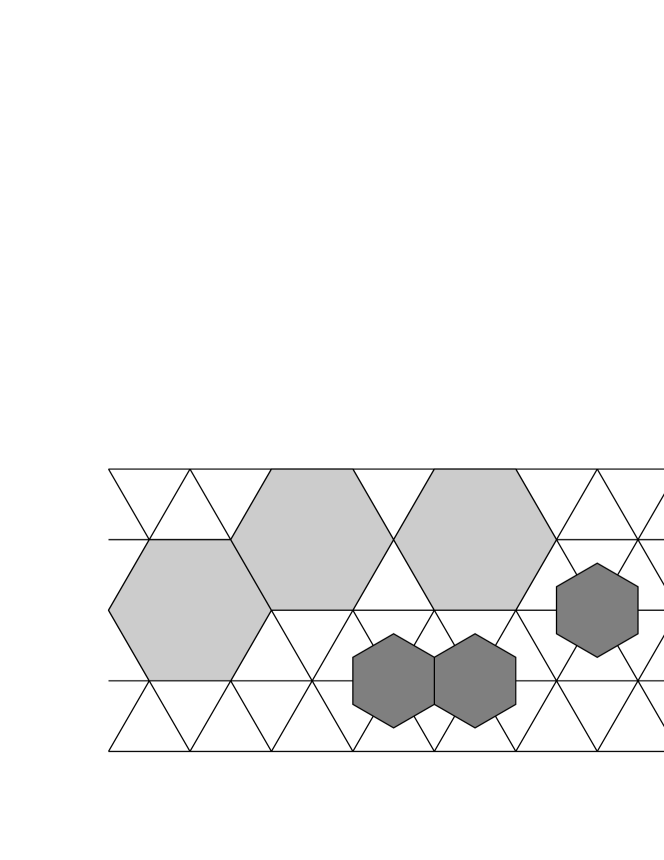
Figure 1: A typical configuration of large and small hexagons.

Figure 2: Phase diagram in the $z_{1}$–$z_{2}$ plane calculated by Van Duijneveldt and Lekkerkerker [7, 8] from Monte Carlo simulations. The letters F, G, L and S indicate the fluid, gas, liquid and solid phase, respectively.

In this paper we study the same model by different methods. Our interest is in the qualitative, rather than quantitative, aspects of the phase diagram. We do not address the general question whether gas–liquid–solid behaviour is possible in binary hard-core mixtures. The paper is organised as follows. First we briefly review the Monte Carlo approach of Van Duijneveldt and Lekkerkerker, and we give some exact results. Then we describe our numerical transfer matrix calculations. Next we discuss the relation of the model with an exactly solvable RSOS model and with the dilute three-state Potts model. Finally we propose an explanation for the discrepancy between our results and those of Van Duijneveldt and Lekkerkerker.

2 Monte Carlo simulation and exact results

Before we review the Monte Carlo method of Van Duijneveldt and Lekkerkerker [7, 8] and discuss some exact results, we make the following notational conventions: the subscripts 1 and 2 refer to the large and small hexagons, respectively; the superscript 0 refers to the pure hard hexagon model; the symbol $N$ without subscript is the number of sites and is generally omitted as an argument of the thermodynamic quantities.

We consider the semi-grand canonical partition function $Z(N_{1},z_{2})$ of large hexagons, whose number $N_{1}$ is fixed, and small hexagons, whose fugacity $z_{2}$ is fixed, on $N$ lattice sites. We may view the small hexagons as causing an effective so-called depletion interaction [13] between the large hexagons. The question is then if this attractive depletion interaction is strong enough to induce a fluid–fluid transition. The effective interaction can be expressed in the number of sites available for small hexagons, once the large hexagons have been placed on the lattice. Interestingly, the sites available for small hexagons are exactly the sites where an additional large hexagon could be inserted. Such sites are called free. It is easy to express the semi-grand canonical partition function $Z(N_{1},z_{2})$ in terms of the canonical partition function $Z^{0}(N_{1})$ of the hard hexagon model and the probability distribution $p(N_{\mathrm{f}}|N_{1})$ for the number $N_{\mathrm{f}}$ of free lattice sites in the hard hexagon model:

$$Z(N_{1},z_{2})=Z^{0}(N_{1})Z^{\prime}(N_{1},z_{2}),$$

where

$$Z^{\prime}(N_{1},z_{2})=\sum_{N_{\mathrm{f}}}\,p(N_{\mathrm{f}}|N_{1})(1+z_{2})^{N_{\mathrm{f}}}.$$

After taking logarithms this gives the free energy:

$$F(N_{1},z_{2})=F^{0}(N_{1})+F^{\prime}(N_{1},z_{2}),$$ (1)

Van Duijneveldt and Lekkerkerker determine the probability distribution $p$ from canonical Monte Carlo simulations of the hard hexagon model. To determine accurately the wings of the distribution an umbrella sampling technique is employed. They calculate $F^{\prime}$ from $p$, and for fixed $z_{2}$ fit a polynomial in $\rho_{1}:\,=N_{1}/N$ to this quantity. They obtain the free energy $F$ from (1), using Baxter’s exact result [11, 12] for $F^{0}$ and the fitted polynomial for $F^{\prime}$. The fugacity $z_{1}$ of the large hexagons and the pressure $P$ are calculated in the usual way from $F$. Finally phase equilibrium is determined by looking for phases with equal $z_{1}$ and $P$ but different $\rho_{1}$. As this calculation is carried out for fixed $z_{2}$, $z_{2}$ is also equal in the phases. The resulting phase diagram is shown in Figure 2. It has three branches: liquid–solid, gas–solid and gas–liquid. The branches meet at the three-phase point, at $z_{1}=22.5$ and $z_{2}=1.89$. (Van Duijneveldt and Lekkerkerker use the term “triple point”, but as that suggests the coexistence of three phases where three first-order transitions meet we prefer to use the term “three-phase point”.) The gas–liquid end-point is located at $z_{1}=13.3$ and $z_{2}=1.36$.

Expanding $Z^{\prime}$ to first order in $z_{2}$ gives:

$$Z^{\prime}(N_{1},z_{2})=1+z_{2}\langle N_{\mathrm{f}}\rangle^{0}_{N_{1}}+o(z_{2}).$$ (2)

For a finite system we could have written ${\cal O}(z_{2}^{2})$ instead of $o(z_{2})$, but in the thermodynamic limit this is not valid at the phase transition of the hard hexagon model. Lekkerkerker (unpublished) found that the average $\rho_{\mathrm{f}}:\,=\langle N_{\mathrm{f}}/N\rangle^{0}_{N_{1}}$ can be calculated exactly, as follows. Adding one hexagon to a configuration of $N_{1}$ hexagons can be done in $N_{\mathrm{f}}$ ways. By doing this to all configurations of $N_{1}$ hexagons each configuration of $N_{1}+1$ hexagons is obtained exactly $N_{1}+1$ times. Hence

$$\langle N_{\mathrm{f}}\rangle^{0}_{N_{1}}Z^{0}(N_{1})=(N_{1}+1)Z^{0}(N_{1}+1),$$

which in the thermodynamic limit yields

$$\rho_{\mathrm{f}}={\rho_{1}\over z_{1}}.$$ (3)

This is an example of Widom’s famous particle-insertion formula [14]. In the Appendix we apply this exact result in the method of Van Duijneveldt and Lekkerkerker. In particular we show that the existence of a Van der Waals loop cannot be concluded from its presence in the first order approximant (2).

As the first derivatives of the thermodynamic functions with respect to $z_{2}$ are known in this way, we shall now attempt to calculate the locus of the phase transition in this order. The difference between the large and small hexagons is, that two small hexagons may occupy neighbouring sites, whereas two large ones may not. At small $z_{2}$ the density of small hexagons is low, so that they will generally occur isolated. Thus they cannot be distinguished from the large ones. For the grand canonical partition function this implies:

$$Z(z_{1},z_{2})=Z^{0}(z_{1}+z_{2})+o(z_{2}).$$ (4)

This suggests that the locus of the phase transition is given by

$$z_{1}=z_{1}^{\mathrm{c}}-z_{2}+o(z_{2}),$$ (5)

where the superscript $\mathrm{c}$ refers to the critical point of the pure hard hexagon model. The particle densities follow also:

$$\rho_{1}(z_{1},z_{2})={z_{1}\over z_{1}+z_{2}}\rho_{1}^{0}(z_{1}+z_{2})+o(z_{2})$$

for the large hexagons, and similarly for the small ones. Combining these results yields the density of the large hexagons at the phase transition:

$$\rho_{1}=\left(1-{z_{2}\over z_{1}^{\mathrm{c}}}\right)\rho_{1}^{\mathrm{c}}+o(z_{2}).$$ (6)

Equations (5) and (6) cannot be derived rigorously from (4) alone, but we conjecture that they are nevertheless valid.

3 Transfer matrix approach

Now we study the model through its row-to-row transfer matrix. For practical reasons, we work with sawtooth rows as shown in Figure 3. One advantage is that the high density ground state of the hexagons fits on the lattice (which has an even number of sites), whereas for straight rows it does so only when the system size is a multiple of three. Another advantage is that the transfer matrix can be built up by repeatedly adding one site, without increasing the total number of sites. Periodic boundary conditions are imposed on the rows. The number of “teeth” is denoted by $W$, so a row contains $2W$ sites and has length $L=W\sqrt{3}$. The largest few eigenvalues of the transfer matrix (in the zero-momentum sector) were calculated numerically for $W=2$, …, $5$, using the power method.

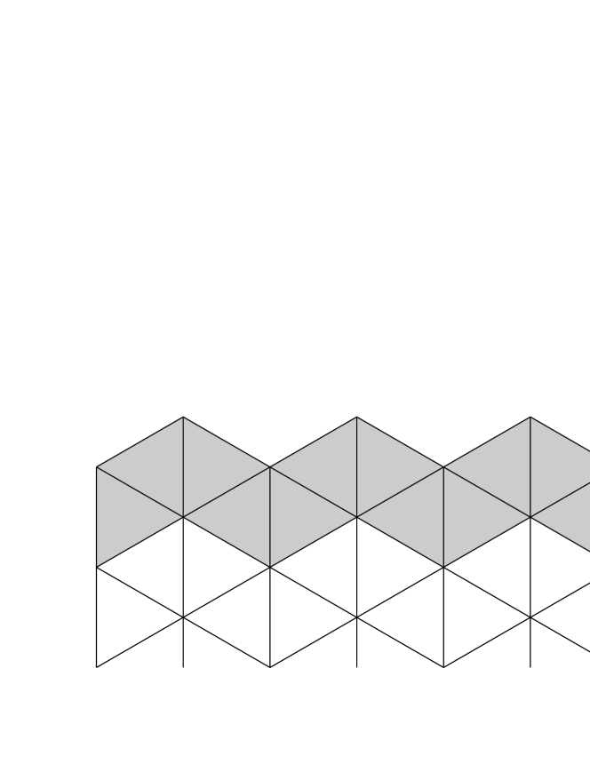
Figure 3: The transfer matrix adds one row (shaded) to the system.

In the ordered regime there are in fact three coexisting ordered phases, corresponding to the three sub-lattices of the triangular lattice. They give rise to three eigenvectors of the transfer matrix, dominated by these ordered phases: one symmetric and two asymmetric for permutations among the ground states. The symmetric vector has the largest eigenvalue $\Lambda_{0}$. The asymmetric vectors have a complex conjugate pair of eigenvalues $\Lambda_{\mathrm{M}}$ and $\Lambda_{\mathrm{M}}^{*}$. In the region of the phase diagram we are interested in, $\Lambda_{0}$, $\Lambda_{\mathrm{M}}$ and $\Lambda_{\mathrm{M}}^{*}$, together with another real eigenvalue $\Lambda_{\mathrm{T}}$, turn out to be the largest eigenvalues of the transfer matrix. The phase behaviour can be diagnosed from the behaviour of the gaps between the eigenvalues, $\Delta_{\mathrm{M}}:\,=\log|\Lambda_{0}/\Lambda_{\mathrm{M}}|$ and $\Delta_{\mathrm{T}}:\,=\log|\Lambda_{0}/\Lambda_{\mathrm{T}}|$, as the system size $L$ tends to infinity.

The gap $\Delta_{\mathrm{T}}$ is an inverse correlation length between density fluctuations. In the absence of a phase transition, the bulk ($L=\infty$) value of this length is finite and the value for finite $L$ approaches this bulk value when $L$ tends to infinity. Hence $\Delta_{\mathrm{T}}$ tends to a non-zero limit. At a critical point the bulk correlation length diverges and the value for finite $L$ is proportional to $L$. As a consequence of scale invariance $\Delta_{\mathrm{T}}$ decreases as $1/L$. At a first-order transition with a change in the density, however, $\Delta_{\mathrm{T}}$ is not an inverse correlation length. The eigenvalues $\Lambda_{0}$ and $\Lambda_{\mathrm{T}}$ are then asymptotically degenerate. Their gap $\Delta_{\mathrm{T}}$ is related to the interfacial tension between the coexisting phases. More precisely, $\Delta_{\mathrm{T}}$ decays as $\exp(-\sigma L)$, where $\sigma$ is proportional to the interfacial tension [15].

For the gap $\Delta_{\mathrm{M}}$ the situation is analogous. In the disordered regime, it is an inverse correlation length, here between fluctuations in the sub-lattice ordering. Thus the gap approaches a non-zero value as $L$ grows. At a first-order transition between two disordered phases this correlation length is generally different in the two phases. Therefore the value of $\Delta_{\mathrm{M}}$ undergoes a sharp change through the transition, approaching a jump as the system size $L$ increases. At a critical point the bulk correlation length diverges, so that $\Delta_{\mathrm{M}}$ decays as $1/L$ when $L$ increases. In the ordered regime three phases coexist, and the eigenvalues $\Lambda_{0}$ and $\Lambda_{\mathrm{M}}$ (and $\Lambda_{\mathrm{M}}^{*}$) are asymptotically degenerate: $\Delta_{\mathrm{M}}$ decays exponentially with $L$. At a first-order transition between an ordered and a disordered phase by the same token $\Delta_{\mathrm{M}}$ vanishes exponentially with $L$.

We shall now distinguish between two scenarios: (i) there are two phases (fluid and solid) as in Figure 4(a); (ii) there are three phases (gas, liquid and solid) as in Figure 4(b). The gaps should behave as follows. At fixed $z_{2}$, the gap $\Delta_{\mathrm{M}}$ decreases with increasing $z_{1}$, whereas $\Delta_{\mathrm{T}}$ has a minimum at the phase transition(s). For low $z_{2}$, see the lower dashed lines in Figures 4(a) and 4(b), the scaled gaps $L\Delta_{\mathrm{M}}$ and $L\Delta_{\mathrm{T}}$ will tend to a non-zero value when $L\to\infty$ at the critical line. For high $z_{2}$, see the upper dashed lines, this is no longer the case: both scaled gaps tend to zero when $L\to\infty$ at the phase transition, which is now first-order. On the middle dashed line in Figure 4(b), $\Delta_{\mathrm{M}}$ changes rapidly at the gas-liquid transition. Furthermore $\Delta_{\mathrm{T}}$ has two minima: at the gas-liquid transition and at the liquid-solid transition. When $L\to\infty$, the minimum of the scaled gap $L\Delta_{\mathrm{T}}$ tends to zero at the gas–liquid transition, but to a non-zero value at the liquid–solid transition. Thus the gas-liquid transition in Figure 4(b) can be recognised from the appearance of a sudden change in $\Delta_{\mathrm{M}}$ and a second minimum of $\Delta_{\mathrm{T}}$.

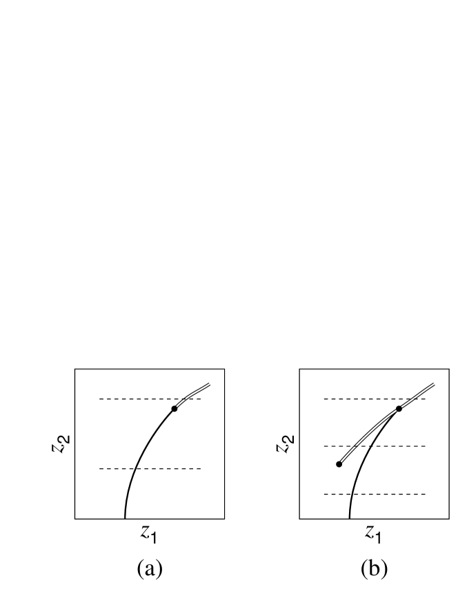
Figure 4: (a) Phase diagram with a fluid and solid phase. The critical line (fat) terminates at a tricritical point where the phase transition becomes first-order (double line). (b) Phase diagram with gas, liquid, and solid phases. The critical line (fat) meets the first-order transition (double line) at the three-phase point.

For $z_{2}=0.0$, $0.1$, …, $3.0$ the scaled gaps $L\Delta_{\mathrm{M}}$ and $L\Delta_{\mathrm{T}}$ were plotted as function of $z_{1}$ for $W=2$ ,…, $5$. Figures 5–8 show examples of this. We found no indication that $\Delta_{\mathrm{T}}$ has two minima. One could argue that two minima might be fused to a single one for these relatively small systems; however, the sharpest and deepest minimum (at the gas–liquid transition) is clearly absent. This pleads against the three-phase scenario in favour of the two-phase scenario. We also saw no sudden change in $\Delta_{\mathrm{M}}$. However, even if a gas–liquid transition were present, the signal in $\Delta_{\mathrm{M}}$ might be hard to detect.

Figure 5: The scaled gaps $L\Delta_{\mathrm{M}}$ as a function of $z_{1}$ on the line $z_{2}=1.7$.

Figure 6: The scaled gaps $L\Delta_{\mathrm{T}}$ as a function of $z_{1}$ on the line $z_{2}=1.7$.

Figure 7: The scaled gaps $L\Delta_{\mathrm{M}}$ as a function of $z_{1}$ on the line $z_{2}=2.3$.

Figure 8: The scaled gaps $L\Delta_{\mathrm{T}}$ as a function of $z_{1}$ on the line $z_{2}=2.3$.

The three-phase scenario can be obtained by introducing an extra parameter into the model. Assign a weight $\kappa$ to every lattice edge joining a small hexagon and an empty site. For $\kappa=1$ one recovers the original model. For $\kappa=0$ any contact between a small particle and an empty site is forbidden. In this limit the model either contains no small hexagons at all or is completely filled with them. The regime without small hexagons still exhibits the hard hexagon transition as long as $1+z_{2}$ is smaller than the partition sum per site of the hard hexagon model. Beyond this value the phase filled with small particles takes over. Thus the ordered and disordered hard hexagon phases meet with the pure small hexagon phase, where the phase transition between them terminates in a three-phase point. For $\kappa$ close to zero the model will still obey the three-phase scenario. Here $\Delta_{\mathrm{T}}$ is indeed found to have two minima, see Figure 9. (The maxima in this figure at first sight seem to be crossings of eigenvalues, but a very close look reveals that they are in fact rounded.) This supports our interpretation of the absence of a second minimum in $\Delta_{\mathrm{T}}$ as evidence against the three-phase scenario.

Figure 9: The scaled gaps $L\Delta_{\mathrm{T}}$ as a function of $z_{1}$ on the line $z_{2}=1.3$ in the model with extra parameter $\kappa=0.6$. The inset shows the deep minima in more detail.

The locus in the $z_{1}$–$z_{2}$ plane of the phase transition can be estimated for example as the location of the minimum of $\Delta_{\mathrm{T}}$. For fixed $z_{2}$ the value of $z_{1}$ at which this gap takes its minimum was determined. The results for $W=5$ and $W=6$ are plotted in Figure 10. In order to obtain the locus in the $\rho_{1}$–$z_{2}$ plane the density of large hexagons was computed using

$$\rho_{1}=z_{1}\frac{\partial}{\partial z_{1}}\left(-\log\Lambda_{0}\right).$$

(It should be noted that for such small $W$ this does not seem to be very accurate.) Figure 11 shows the result. We observed that for fixed $z_{2}$ the graphs of $\rho_{1}$ versus $z_{1}$ for different system sizes pass approximately through one point. One could ask whether this is the critical point, as would be the case in a self-dual model. The locus of the intersection of the graphs for $W=5$ and $W=6$ is shown in Figure 11. Figures 10 and 11 also show the phase diagrams given by Van Duijneveldt and Lekkerkerker [8].

Figure 10: Locus in the $z_{1}$–$z_{2}$ plane of the minimum of the gap $\Delta_{\mathrm{T}}$ for $W=5$ ($+$) and $W=6$ ($\times$) and phase diagram of Van Duijneveldt and Lekkerkerker (solid line). The asymptote (5) is also shown.

Figure 11: Locus in the $\rho_{1}$–$z_{2}$ plane of phase transition calculated from $W=5$ ($+$) and $W=6$ ($\times$), locus of the intersection of the graphs for $W=5$ and $W=6$ of $\rho_{1}$ versus $z_{1}$ ($\odot$), and phase diagram of Van Duijneveldt and Lekkerkerker (solid line). The asymptote (6) is also shown.

First-order and second-order transitions are not easily distinguished from each other by the numerical data. In both cases $\Delta_{\mathrm{T}}$ has a minimum, only the dependence on $L$ of the depth of the minimum is different. For $z_{2}=1.7$, the graphs of the $L\Delta_{\mathrm{M}}$ pass approximately through one point, see Figure 5. The $L\Delta_{\mathrm{T}}$ have a minimum that increases slowly with $L$ and may converge to a non-zero value, see Figure 6. This points to a second-order transition. For $z_{2}=2.3$, the graphs of $L\Delta_{\mathrm{M}}$ do not pass neatly through one point, see Figure 7. The minimum of $L\Delta_{\mathrm{T}}$ decreases with $L$ and may vanish asymptotically, see Figure 8. This points to a first-order transition. The behaviour of $L\Delta_{\mathrm{M}}$ and $L\Delta_{\mathrm{T}}$ changes gradually between $z_{2}=1.7$ and $z_{2}=2.3$. Thus the value of $z_{2}$ at the tricritical point is estimated roughly to lie between 1.7 and 2.3.

By universality the limit values of $L\Delta_{\mathrm{M}}$ and $L\Delta_{\mathrm{T}}$ at the phase transition are $2\pi x_{\mathrm{M}}$ and $2\pi x_{\mathrm{T}}$ respectively, with $x_{\mathrm{M}}=2/15$ and $x_{\mathrm{T}}=4/5$ on the hard hexagon critical line ($c=4/5$), and $x_{\mathrm{M}}=2/21$ and $x_{\mathrm{T}}=2/7$ at the hard hexagon tricritical point ($c=6/7$), see for instance [16]. On the critical line close to the critical point one expects to find the tricritical values for small system sizes, but the critical values for large sizes. The limits were also estimated from the graphs of $L\Delta_{\mathrm{M}}$ and $L\Delta_{\mathrm{T}}$ for $z_{2}=0.0$ (not shown) and $z_{2}=1.7$. For $z_{2}=0.0$ we found $x_{\mathrm{M}}\approx 0.14$ and $x_{\mathrm{T}}\approx 0.80$. This is in good agreement with the critical values $x_{\mathrm{M}}=2/15$ and $x_{\mathrm{T}}=4/5$. For $z_{2}=1.7$ we found $x_{\mathrm{M}}\approx 0.13$ and $x_{\mathrm{T}}\approx 0.3$. This agrees reasonably with the tricritical values $x_{\mathrm{M}}=2/21$ and $x_{\mathrm{T}}=2/7$, which are expected for small system size near the tricritical point.

4 Relation to an $A_{2}^{(2)}$ RSOS model

Some properties of the large-and-small hexagon model it has in common with an exactly solvable model. In order to make use of the exact solution we investigate if the two models are ever parametrically close. The sites of the large-and-small hexagon model can be in three states: 0 (empty), 1 (large hexagon), or 2 (small hexagon). For neighbouring sites the combinations 1–1 and 1–2 are excluded. The same is true for the $L=7$ case of the exactly solvable $A_{2}^{(2)}$ restricted solid-on-solid model of Kuniba [17, 18]. This is an interaction-round-a-face model on the square lattice. For a suitable choice of its spectral parameter, the condition on neighbouring sites extends to one of the diagonals of the square face. The Boltzmann weight of the square face then factors into weights of the composing triangles:

$$W\pmatrix{d&c\cr a&b\crcr}=W\pmatrix{d&\cr a&b\crcr}W\pmatrix{d&c\cr&b\crcr}$$

and these triangle weights are invariant under rotation:

$$W\pmatrix{c&\cr a&b\crcr}=W\pmatrix{c&b\cr&a\crcr}=W\pmatrix{b&\cr c&a\crcr}=W\pmatrix{b&a\cr&c\crcr}=W\pmatrix{a&\cr b&c\crcr}=W\pmatrix{a&c\cr&b\crcr},$$

so that the model is isotropic on the triangular lattice. The model still has one parameter (the elliptic nome), but this solvable line stays away from our phase diagram. For example at the critical point the triangle weights are

$$W\pmatrix{0&\cr 0&0\crcr} = 1,$$

$$W\pmatrix{0&\cr 1&0\crcr} = 4.412,$$

$$W\pmatrix{0&\cr 2&0\crcr} = 3.903,$$

$$W\pmatrix{0&\cr 2&2\crcr} = 3.129,$$

$$W\pmatrix{2&\cr 2&2\crcr} = 3.761,$$

which is not of the form

$$W\pmatrix{0&\cr 0&0\crcr} = 1,$$

$$W\pmatrix{0&\cr 1&0\crcr} = z_{1}^{1/6},$$

$$W\pmatrix{0&\cr 2&0\crcr} = z_{2}^{1/6},$$

$$W\pmatrix{0&\cr 2&2\crcr} = z_{2}^{1/3},$$

$$W\pmatrix{2&\cr 2&2\crcr} = z_{2}^{1/2}.$$

Application of the numerical transfer matrix method from Section 3 to this critical model shows that it is in the tricritical three-state Potts universality class.

5 Relation to the dilute three-state Potts model

The large-and-small hexagon model is intimately related to the dilute three-state Potts model [19]. Because this relation gives insight in the phase diagram we will consider it here in more detail. On every site $j$ of a two-dimensional lattice with coordination number $v$ lives a variable $s_{j}$ that can take the values 0, 1, 2, 3. Of these the states $s_{j}>0$ take the role of local occupancy of one of the three sub-lattices of the hard hexagon model, and the state $s_{j}=0$ is neutral or vacant. The Hamiltonian of the dilute Potts model is

$${\cal H}=-\sum_{<j,k>}\left(\delta_{s_{j},s_{k}}+K\delta_{s_{j},0}\delta_{s_{k},0}\right)-L\sum_{j}\delta_{s_{j},0},$$ (7)

where the first sum is over nearest neighbour pairs of sites. In the parameter space $(K,L,T)$ the model has a line of tricritical points as well as a line of critical-end-points [19], see Figure 12. As we will argue below, it is fairly clear where these come together, namely in the critical point of the four-state Potts model, $K=0$, $L=0$ and $T=T_{\mathrm{c}}$, where all the four states are treated identically.

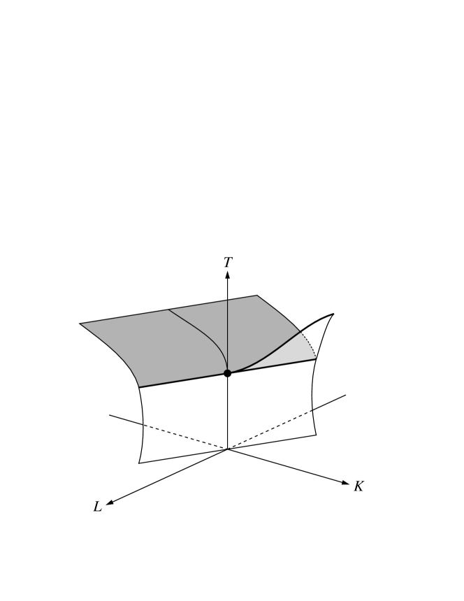
Figure 12: A qualitative picture of the phase diagram of the dilute three-state Potts model. The dense coexistence region (back) and the dilute region (front) are separated by the three-state Potts critical surface (shaded) and the lower part of the first-order surface (not shaded). These surfaces meet at a line of three-state Potts tricritical points (left) and a line of three-state Potts critical-end-points (right). The upper part of the first-order surface (not shaded) separates a dilute and a dense disordered phase. It is bounded by a line of Ising critical points. The fat dot indicates the four-state Potts critical point.

At $T=0$ there is a dilute phase with $s_{j}=0$ when $vK+2L>0$, while the three dense, or ordered phases associated with $s_{j}=1,2,3$ coexist when $vK+2L<0$. These phases extend to non-zero temperatures so that a first-order surface separates the dilute region from the dense coexistence region. This first-order surface will not remain precisely at $vK+2L=0$ for $T>0$, but by symmetry it does include the $T$-axis, $K=L=0$. At high temperature the coexistence region is bounded by a surface of three-state Potts critical points, shaded gray in Figure 12, where the line tension between the coexisting dense phases vanishes. This critical sheet must join with the first-order surface in a line of multicritical points, as they both form boundaries to the coexistence region.

The nature of this multicritical line depends on the sign of $K$, as follows. Along the first-order sheet we can distinguish two line tensions, namely that between two different dense phases, and that between a dense and the dilute phase. When $K<0$ the interface between the dilute and the dense phases costs less energy than that between two of the dense phases. However on the critical surface the line tension between the dense phases vanishes. As a consequence all line tensions vanish simultaneously where the critical and first-order sheets meet as $K<0$. The separatrix between these two types of phase transition is thus a tricritical line. When $K>0$ the dense–dense interface costs less energy than the dense–dilute interface, so there remains a positive line tension between the dilute phase and the dense phases where the first-order sheet meets the critical surface, and the dense–dense interfacial tension vanishes. This results in a critical-end-point scenario: The three-state Potts critical sheet terminates where it hits the first-order sheet. The first-order sheet extends beyond this line, separating a disordered dense phase from the dilute phase. Obviously, at $K=0$ the two scenarios come together, and we conclude that the tricritical curve and the critical-end curve as well as the critical line terminating the dilute–disordered phase transition all meet in the four-state Potts critical point, marked as a dot in Figure 12. This qualitative description of the phase diagram of (7), though not rigorous, is the simplest possible scenario, and has been corroborated by numerical studies [19].

These considerations are of interest for the large-and-small hexagon model because that can be mapped onto a model sufficiently similar to the dilute Potts Hamiltonian (7) that the arguments can be carried over. We divide the triangular lattice into triangular blocks of three sites each, indicated in Figure 13(a). Each block then has three sites which we label 1, 2, and 3. We assign a spin variable $s_{j}$ to each block, as follows. When the site $\sigma$ in block $j$ is occupied by a large hexagon, the spin variable takes the value $s_{j}=\sigma$, while in all other cases $s_{j}=0$. For convenience of notation we consider one block variable $s_{0}$, in interaction with six neighbours $s_{j}$ with $1\leq|j|\leq 3$, as shown in Figure 13(a). The blocks $j$ with $j>0$ contain two sites neighbouring the site $j$ of the central block, and the block $-j$ sits in the opposite direction. To give an expression for the interaction we introduce the variables

$$p_{i}=\left(\delta_{s_{i},0}+\delta_{s_{i},i}\right)\left(1-\delta_{s_{-j},j}\right)\left(1-\delta_{s_{-k},k}\right),$$ (8)

where $i,j,k$ is a permutation of $1,2,3$. Note that $p_{i}$ can only take the values 0 and 1, and it signals if site $i$ of the central block is free. The spin states 1, 2, and 3 have weight $z_{1}$, but are excluded by some configurations of the neighbouring blocks by the factor

$$\left[1-\delta_{s_{0},j}(1-p_{j})\right].$$ (9)

In other words the state $s_{0}=j$ is not allowed when $p_{j}=0$. The weight of the spin state $s_{0}=0$ depends on the surrounding blocks and is given by the expression

$$(1+z_{2})^{p_{1}+p_{2}+p_{3}}.$$ (10)

If this model would be precisely the dilute Potts model with Hamiltonian (7) we could simply read off the value of $K$ and its sign would conclusively decide between a tricritical point versus a three phase point. The interaction is of course much more complicated than that of the dilute Potts model, but the overall effect is that some combinations of unequal nearest neighbours are excluded or suppressed. As the state 0 is treated altogether different from the states 1, 2, and 3, it is difficult to judge the sign of the effective coupling $K$ in (7).

Figure 13: (a) The large-and-small hexagon model can be mapped onto a Potts-like model by grouping the sites into blocks of three. The numbers indicate the labelling of blocks and of the sites within the blocks. (b) The big hexagon model can be mapped onto a Potts-like model by dividing the sites into blocks of four. The numbers indicate the labelling of the sites within the blocks. The blocks are numbered as in (a).

However, this problem can be resolved because there is a model in the universality class and with the symmetry of the four-state Potts model which can be mapped to a very similar model. Consider a one-species lattice gas on the triangular lattice in which not only first neighbours but also second neighbours (at distance $\sqrt{3}$) can not be occupied simultaneously. We will refer to this model as the big hexagon model. For large values of the fugacity $z$ this model will be in an ordered phase in which one out of four sub-lattices is occupied preferentially. At low fugacity the symmetry between the sub-lattices is unbroken. The phase transition is known to be in the four-state Potts universality class from the symmetry of its Landau–Ginzburg–Wilson Hamiltonian [20, 21]. We are not aware of studies giving the critical fugacity of this model, but we have seen numerically that it is about half the value of the hard hexagon model.

The big hexagon model can be mapped exactly onto a Potts-like model very similar to the model above, as expressed in (9) and (10). Now we take blocks of four sites as shown in Figure 13(b), one in each sub-lattice. It is convenient to label the spins in each block by the numbers 0, 1, 2, 3 as indicated. When the site $j$ in a block is occupied, the block variable takes the value $j$. In addition, when none of the sites are occupied, the block variable is taken to be 0. Therefore the weight of the states $j>0$ is $z$ and the weight of state 0 will again depend on the states of the neighbouring blocks. We again consider a block variable $s_{0}$ interacting with its neighbours, which are labelled in the same way as in the previous case. We will use again variables $p_{i}$ defined by (8). The central site of the block 0 is free if and only if $p_{1}=p_{2}=p_{3}=1$. Some combinations of states of neighbouring blocks are excluded, described by precisely the same expression (9) as before. However, also some combinations of next-neighbouring blocks are excluded. For example site $j$ of block $-j$ and site $k$ of block $-k$ in Figure 13(b) are second neighbours, so the combination $s_{-j}=j$ and $s_{-k}=k$ is excluded. We introduce a variable

$$q=1-\delta_{s_{-1},1}\delta_{s_{-2},2}-\delta_{s_{-2},2}\delta_{s_{-3},3}-\delta_{s_{-3},3}\delta_{s_{-1},1}+2\delta_{s_{-1},1}\delta_{s_{-2},2}\delta_{s_{-3},3}.$$

Note that $q$ can only take the values 0 and 1; it signals if there are no pairs $s_{-j}=j$ and $s_{-k}=k$. If $s_{0}\neq 0$ then $s_{-j}=j$ or $s_{-k}=k$ is already excluded by the interaction between the neighbouring blocks 0 and $-j$ or $-k$. Therefore the exclusion of the combination $s_{-j}=j$ and $s_{-k}=k$ can be taken into account by including a factor $q$ in the weight of block 0 in state 0. This weight is then given by

$$q(1+z)^{p_{1}p_{2}p_{3}}.$$ (11)

In this way any exclusion between sites of next-neighbouring blocks is absorbed in the weight of state 0 of the intervening block.

This resulting model is strikingly similar to the Potts-like model above. The exclusion rules for pairs of neighbouring blocks are identical and when we choose $z_{1}=z$, the weight of the spin states 1, 2, and 3 is the same. In both models the weight of the state 0 depends on the configuration of its six neighbours, via expression (10) and (11), respectively. When we further specify $(1+z_{2})^{3}=(1+z)$ the weights for $s_{0}=0$ are equal in the case that $p_{1}=p_{2}=p_{3}$ and $q=1$. In particular they are equal when the surrounding blocks are also in state 0, because then $p_{1}=p_{2}=p_{3}=1$ and $q=1$.

It is the exclusion and suppression of configurations with unequal neighbours which determines an effective temperature $T$ and coupling $K$ in (7). The large-and-small hexagon model and the big hexagon model with the parameters as set above will have the same effective temperature $T$, as all configurations involving only spin states $s>0$ have the same weight between the two models. Only when a block has $s=0$, while one or more of its neighbours have $s>0$, the configurational weights between the two models can be different. In all such cases the weight in the big hexagon model is smaller than that in the large-and-small hexagon model, which is easy to see from direct comparison of the expressions (10) and (11). Therefore we can confidently claim that the effective coupling $K$ is the greater in the big hexagon model, as configurations with unequal neighbours of which one $s=0$ are more strongly suppressed than in the large-and-small hexagon model. However, since the big hexagon model has the symmetry of the four-state Potts model, clearly its effective coupling $K=0$. Therefore the effective $K$ in the large-and-small hexagon model is necessarily negative, which, as argued above, results in a tricritical scenario.

6 Discussion

The results of our transfer matrix calculations provide evidence against the three-phase scenario of Figure 4(b) in favour of the two-phase scenario of Figure 4(a). This contradicts the earlier findings of Van Duijneveldt and Lekkerkerker [7, 8]. We propose the following explanation. Van Duijneveldt and Lekkerkerker effectively calculate the free energy difference between the binary mixture and the pure hard hexagons. They then look for phases of equal pressure and fugacities but different composition. They do not calculate the order parameter for the mixture. Their method has some drawbacks. Firstly, it cannot detect second-order transitions, because these do not involve a jump in the particle densities. Secondly, it uses a polynomial fit for the free energy difference, so that the total free energy still seems to possess the singularity of the pure hard hexagon model. Thirdly, whether $P$ exhibits a Van der Waals loop or not may depend sensitively on $p(N_{\mathrm{f}}|N_{1})$. Thus the locus of the liquid–solid branch in their phase diagram is a spurious consequence of the implicit assumption that the ordering transition remains at fixed $\rho_{1}$ for small values of $z_{2}$. Their qualitative conclusion that a gas–liquid transition is present relies on quantitative properties of the calculated phase diagram, viz. the locations of the various branches. Figure 10 suggests that their gas–liquid and gas–solid branch together form the true fluid–solid line and that the critical point of their gas–liquid branch is in fact the tricritical point. This agrees well with the fact that Figures 10 and 11 show enhanced size dependence of the phase diagram near their gas–liquid critical point. However, this point is located at $z_{2}=1.36$ (and $z_{1}=22.5$), whereas we estimate roughly $1.7<z_{2}<2.3$ for the tricritical point. Being unable to present a satisfactory explanation for this discrepancy, we stress that our data do not signal a clearly determined locus of the tricritical point. It should also be noted that in our transfer matrix calculations only very small system sizes have been considered. Going to significantly larger systems might allow for more definitive quantitative statements, but this requires much greater computational resources.

Other evidence comes from the relation with the dilute three-state Potts model. The large-and-small hexagon model can be mapped onto a Potts-like model. Another model, the big hexagon model, whose phase behaviour is known, can also be mapped onto a Potts-like model. A comparison of the effective temperature and coupling constants between the large-and-small hexagon model on the one hand and the big hexagon model on the other hand indicates that the large-and-small hexagon model should follow the two-phase scenario.

Acknowledgement

We thank Jeroen van Duijneveldt and Henk Lekkerkerker for useful discussions. The former kindly provided data used in making Figures 10 and 11. This work was supported by the foundation Fundamenteel Onderzoek der Materie.

Appendix

It is instructive to follow the method of Van Duijneveldt and Lekkerkerker using (2) and (3) instead of Monte Carlo results. Calculating the pressure from (2) gives

$$P=P^{0}+\left(\rho_{\mathrm{f}}-{\mathrm{d}\rho_{\mathrm{f}}\over\mathrm{d}\rho_{1}}\right)z_{2}+o(z_{2}).$$ (12)

Baxter [12, p. 451] lists expansions around the critical point of several thermodynamic quantities of the pure hard hexagon model. Combining these expansions with (3) and (12) yields

$$P = \left\{P^{\mathrm{c}}+{25(\sqrt{5}-1)\over 2\root 4 \of{5}}\mathop{\rm sgn}(\rho_{1}-\rho_{1}^{\mathrm{c}})|\rho_{1}-\rho_{1}^{\mathrm{c}}|^{3/2}+{\cal O}\left((\rho_{1}-\rho_{1}^{\mathrm{c}})^{2}\right)\right\}$$ (13)

$$+\;\left\{{125\root 4 \of{5}(\rho_{1}^{\mathrm{c}})^{2}\over 2z_{1}^{\mathrm{c}}}|\rho_{1}-\rho_{1}^{\mathrm{c}}|^{1/2}+{\cal O}(\rho_{1}-\rho_{1}^{\mathrm{c}})\right\}z_{2}\;+\;o(z_{2}).$$

This suggests that for small non-zero values of $z_{2}$ the pressure $P$ would exhibit a Van der Waals loop, so that the transition becomes first-order as soon as $z_{2}$ becomes non-zero. That this argument is not valid can be seen by considering for example

$$f_{z}(x)=(x-z)^{3},$$

which we view as a function of $x$, parametrically dependent on $z$. Expanding $f$ to first order in $z$ gives

$$f_{z}(x)=x^{3}-3x^{2}z+o(z)$$

and for all non-zero values of $z$ the function $x^{3}-3x^{2}z$ of $x$ is decreasing between $x=0$ and $x=2z$. It is, however, a first order approximant of $f_{z}(x)$, which for all values of $z$ is an increasing function of $x$.

References

- [1] W. W. Wood and J. D. Jacobson, J. Chem. Phys. 27, 1207 (1957).
- [2] B. J. Alder and T. E. Wainwright, J. Chem. Phys. 27, 1208 (1957).
- [3] W. G. Hoover and F. H. Ree, J. Chem. Phys. 49, 3609 (1968).
- [4] M. D. Eldridge, P. A. Madden, and D. Frenkel, Mol. Phys. 79, 105 (1993).
- [5] J. L. Lebowitz and J. S. Rowlinson, J. Chem. Phys. 41, 133 (1964).
- [6] T. Biben and J.-P. Hansen, Phys. Rev. Lett. 66, 2215 (1991).
- [7] J. S. van Duijneveldt and H. N. W. Lekkerkerker, Phys. Rev. Lett. 71, 4264 (1993).
- [8] J. S. van Duijneveldt and H. N. W. Lekkerkerker, J. Stat. Phys. 78, 103 (1995).
- [9] D. Frenkel and A. A. Louis, Phys. Rev. Lett. 68, 3363 (1992).
- [10] D. M. Burley, Proc. Phys. Soc. 75, 262 (1960).
- [11] R. J. Baxter, J. Phys. A: Math. Gen. 13, L61 (1980).
- [12] R. J. Baxter, Exactly Solved Models in Statistical Mechanics, chapter 14, Academic Press, London, 1982.
- [13] S. Asakura and F. Oosawa, J. Chem. Phys. 22, 1255 (1954).
- [14] B. Widom, J. Chem. Phys. 39, 2808 (1963).
- [15] M. E. Fisher, J. Phys. Soc. Japan (Suppl.) 26, 87 (1969), Proceedings of the International Conference on Statistical Mechanics 1968.
- [16] D. Friedan, Z. Qiu, and S. Shenker, Phys. Rev. Lett. 52, 1575 (1984).
- [17] A. Kuniba, Nucl. Phys. B355, 801 (1991).
- [18] A. Kuniba, private communication.
- [19] A. N. Berker, S. Ostlund, and F. A. Putnam, Phys. Rev. B 17, 3650 (1978).
- [20] E. Domany, M. Schick, and J. S. Walker, Phys. Rev. Lett. 38, 1148 (1977).
- [21] E. Domany, M. Schick, J. S. Walker, and R. B. Griffiths, Phys. Rev. B 18, 2209 (1978).