The statistical properties of the volatility of price fluctuations

Abstract

We study the statistical properties of volatility—a measure of how much the market is likely to fluctuate. We estimate the volatility by the local average of the absolute price changes. We analyze (a) the S&P 500 stock index for the 13-year period Jan 1984 to Dec 1996 and (b) the market capitalizations of the largest 500 companies registered in the Trades and Quotes data base, documenting all trades for all the securities listed in the three major stock exchanges in the US for the 2-year period Jan 1994 to Dec 1995. For the S&P 500 index, the probability density function of the volatility can be fit with a log-normal form in the center. However, the asymptotic behavior is better described by a power-law distribution characterized by an exponent $1+\mu\approx 4$. For individual companies, we find a similar power law asymptotic behavior of the probability distribution of volatility with exponent $1+\mu\approx 4$. In addition, we find that the volatility distribution scales for a range of time intervals. Further, we study the correlation function of the volatility and find power law decay with long persistence for the S&P 500 index and the individual companies with a crossover at approximately $1.5$ days. To quantify the power-law correlations, we apply power spectrum analysis and a recently-developed modified root-mean-square analysis, termed detrended fluctuation analysis (DFA). For the S&P 500 stock index, DFA estimates for the exponents characterizing the power law correlations are $\alpha_{1}=0.66$ for short time scales (within $\approx 1.5\,$days) and $\alpha_{2}=0.93$ for longer time scales (up to a year). For individual companies, we find $\alpha_{1}=0.60$ and $\alpha_{2}=0.74$, respectively. The power spectrum gives consistent estimates of the two power-law exponents.

I Introduction

Physicists are increasingly interested in economic time series analysis for several reasons, among which are the following: (i) Economic time series, such as stock market indices or currency exchange rates, depend on the evolution of a large number of interacting systems, and so is an example of complex evolving systems widely studied in physics. (ii) The recent availability of large amounts of data allows the study of economic time series with a high accuracy on a wide range of time scales varying from $\approx 1$ minute up to $\approx 1\,$year. Consequently, a large number of methods developed in statistical physics have been applied to characterize the time evolution of stock prices and foreign exchange rates [1, 2, 3, 4, 5, 6, 7, 8, 9, 10, 11, 12, 13].

Previous studies [1, 2, 3, 4, 5, 6, 7, 8, 9, 10, 11, 12, 13, 14, 15, 16, 17, 18, 19, 20, 21, 22, 23, 24] show that the stochastic process underlying price changes is characterized by several features. The distribution of price changes has pronounced tails [1, 2, 3, 10, 11, 12, 13, 14] in contrast to a Gaussian distribution. The autocorrelation function of price changes decays exponentially with a characteristic time of approximately $4\,$min. However, recent studies [14, 15, 16, 17, 18, 19, 20, 21] show that the amplitude of price changes, measured by the absolute value or the square, shows power law correlations with long-range persistence up to several months. These long-range dependencies are better modeled by defining a “subsidiary process” [14, 15, 16, 17], often referred to as the volatility in economic literature. The volatility of stock price changes is a measure of how much the market is liable to fluctuate. The first step is to construct an estimator for the volatility. Here, we estimate the volatility as the local average of the absolute price changes.

Understanding the statistical properties of the volatility also has important practical implications. Volatility is of interest to traders because it quantifies the risk [1] and is the key input of virtually all option pricing models, including the classic Black and Scholes model and the Cox, Ross, and Rubinstein binomial models that are based on estimates of the asset’s volatility over the remaining life of the option [25, 26]. Without an efficient volatility estimate, it would be difficult for traders to identify situations in which options appear to be under-priced or overpriced.

We focus on two basic statistical properties of the volatility—the probability distribution function and the two-point autocorrelation function. The paper is organized as follows. In Section 2, we briefly describe the databases used in this study, the S&P 500 stock index and individual company stock prices. In Section 3, we discuss the quantification of volatility. In Section 4, the probability distribution function is studied, and in Section 5, the volatility correlations are studied. The appendix briefly describes a recently-developed method, called detrended fluctuation analysis (DFA) that we use to quantify power-law correlations.

II Data analyzed

A S&P 500 stock index

The S&P 500 index from the New York Stock Exchange (NYSE) consists of 500 companies chosen for their market size, liquidity, and industry group representation in the US. It is a market-value weighted index, i.e., each stock is weighted proportional to its stock price times number of shares outstanding. The S&P 500 index is one of the most widely used benchmarks of U.S. equity performance. We analyze the S&P 500 historical data, for the 13-year period Jan 1984 to Dec 1996 (Fig. 1(a)) with a recording frequency of $15$ seconds intervals. The total number of data points in this 13-year period exceed 4.5 million, and allows for a detailed statistical analysis.

B Individual company stocks

We also analyze the Trades and Quotes (TAQ) database which documents every trade for all the securities listed in the three major US stock markets—the New York Stock Exchange (NYSE), the American Stock Exchange (AMEX), and the National Association of Securities Dealers Automated Quotation (NASDAQ)—for the 2-year period from Jan. 1994 to Dec. 1995 [27]. We study the market capitalizations [28] for the 500 largest companies, ranked according to the market capitalization on Jan. 1 1994. The S&P500 index at anytime is approximately the sum of market capitalizations of these 500 companies[29]. The total number of data points analyzed exceed 20 million.

III Quantifying Volatility

The term volatility represents a generic measure of the magnitude of market fluctuations. Thus, many different quantitative definitions of volatility are use in the literature. In this study, we focus on one of these measures by estimating the volatility as the local average of absolute price changes over a suitable time interval $T$, which is an adjustable parameter of our estimate.

Fig. 1(a) shows the S&P 500 index $Z(t)$ from 1984 to 1996 in semi-log scale. We define the price change $G(t)$ as the change in the logarithm of the index,

$$G(t)\equiv\ln Z(t+\Delta t)-\ln Z(t)\cong\frac{Z(t+\Delta t)-Z(t)}{Z(t)}\;,$$ (1)

where $\Delta t$ is the sampling time interval. In the limit of small changes in $Z(t)$ is approximately the relative change, defined by the second equality. We only count time during opening hours of the stock market, and remove the nights, weekends and holidays from the data set, i.e., the closing and the next opening of the market is considered to be continuous.

The absolute value of $G(t)$ describes the amplitude of the fluctuation, as shown in Fig. 1(b). In comparison to Fig. 1(a), Fig. 1(b) does not show visible global trends due to the logarithmic difference. The large values of $|G(t)|$ correspond to the crashes and big rallies.

We define the volatility as the average of $|G(t)|$ over a time window $T=n\cdot\Delta t$, i.e.,

$$V_{T}(t)\equiv{1\over n}\sum_{t^{\prime}=t}^{t+n-1}|G(t^{\prime})|\;,$$ (2)

where $n$ is an integer. The above definition can be generalized [21] by replacing $|G(t)|$ with $|G(t)|^{\gamma}$, where $\gamma>1$ gives more weight to the large values of $|G(t)|$ and $0<\gamma<1$ weights the small values of $|G(t)|$.

There are two parameters in this definition of volatility, $\Delta t$ and $n$. The parameter $\Delta t$ is the sampling time interval for the data and the parameter $n$ is the moving average window size. Note that the definition of the volatility has an intrinsic error associated with it. In principle, the larger the choice of time interval $T$, the more accurate the volatility estimation. However, a large value of $T$ also implies poor resolution in time.

Fig. 2 shows the calculated volatility $V_{T}(t)$ for a large averaging window $T=8190\,$min (about 1 month) with $\Delta t=30\,$min. The volatility fluctuates strongly during the crash of ’87. We also note that periods of high volatility are not sparse but tend to “cluster”. This clustering is especially marked around the ’87 crash. The oscillatory patterns before the crash could be possible precursors (possibly related to the oscillatory patterns postulated in [7, 8]). Clustering also occurs in other periods, e.g. in the second half of ’90. There are also extended periods where the volatility remains at a rather low level, e.g. the years of ’85 and ’93.

IV Volatility distribution

A Volatility distribution of the S&P 500 index

1 Center part of the distribution

Fig. 3(a) shows the probability density function $P(V_{T})$ of the volatility for several values of $T$ with $\Delta t=30\,$min. The central part shows a quadratic behavior on a log-log scale (Fig. 3(a)), consistent with a log-normal distribution [20]. To test this possibility, the appropriately-scaled distribution of the volatility is plotted on a log-log plot (Fig. 3(b)). The distributions of volatility $V_{T}$, for various choices of $T$ (from $T=120$ min up to $T=900$ min), collapse onto one curve and are well fit in the center by a quadratic function on a log-log scale. Since the central limit theorem holds also for correlated series [30], with a slower convergence than for non-correlated processes [1, 11, 18], in the limit of large values of $T$, one expects that $P(V_{T})$ becomes Gaussian. However, a log-normal distribution fits the data better than a Gaussian, as is evident in Fig. 4 which compares the best log-normal fit with the best Gaussian fit for the data [20]. The apparent scaling behavior of volatility distribution could be attributed to the long persistence of its autocorrelation function [18] (Section 5).

2 Tail of the distribution

Although the log-normal seems to describe well the center part of the volatility distribution, Fig. 3(a) suggests that the distribution of the volatility has quite different behavior in the tail. Since our time window $T$ for estimating volatility is quite large, it is difficult to obtain significant statistics for the tail. Recent studies of the distribution for price changes report power law asymptotic behavior [10, 14, 24]. Since the volatility is the local average of the absolute price changes, it is possible that a similar power law asymptotic behavior might characterize the distribution of the volatility. Hence we reduce the time window $T$ and focus on the “tail” of the volatility.

We compute the cumulative distribution of the volatility. Eq. (2) for different time scales, Fig. 5(a). We find that the cumulative distribution of the volatility is consistent with a power law asymptotic behavior,

$$P(V_{T}>x)\sim{1\over x^{\mu}}\,.$$ (3)

Regression fits yield estimates $\mu=3.10\pm 0.08$ for $T=32\,$min with $\Delta t=1\,$min, well outside the stable Lévy range $0<\mu<2$.

For larger time scales the asymptotic behavior is difficult to estimate because of poor statistics at the tails. In view of the power law asymptotic behavior for the volatility distribution, the drop-off of $P(V_{T})$ for low values of the volatility could be regarded as a truncation to the power law behavior, as opposed to a log-normal.

B Volatility distribution for individual companies

In this section, we extend the investigation of the nature of this distribution to the individual companies comprising the S&P 500, where the amount of data is much larger, which allows for better sampling of the tails.

From the TAQ data base, we analyze 500 time series $S_{i}(t)$, where $S_{i}$ is the market capitalization of company $i$ (i.e., the stock price multiplied with the number of outstanding shares), $i=1,\dots,500$ is the rank in descending order of the company according to its market capitalization on 1 Jan. 1994 and the sampling time is 5 min.The basic quantity studied for individual stocks is the change in logarithm of the market capitalization for each company,

$$G_{i}(t)\equiv\ln S_{i}(t+\Delta t)-\ln S_{i}(t)\cong{S_{i}(t+\Delta t)-S_{i}(t)\over S_{i}(t)}\;,$$ (4)

where the $S_{i}$ denotes the market capitalization of stock $i=1,\dots,500$ and $\Delta t=5\,$min.

As before, we estimate the volatility at a given time by averaging $|G_{i}(t)|$ over a time window $T=n\cdot\Delta t$,

$$V^{i}_{T}\equiv V^{i}_{T}(t)\equiv{1\over n}\sum_{t^{\prime}=t}^{t+n-1}|G_{i}(t^{\prime})|\;.$$ (5)

A normalized volatility is then defined for each company,

$$v^{i}_{T}\equiv v^{i}_{T}(t)\equiv\frac{V^{i}_{T}}{\sqrt{\langle[V^{i}_{T}]^{2}\rangle-\langle V^{i}_{T}\rangle^{2}}}\;,$$ (6)

where $\langle\dots\rangle$ denotes the time average estimated by non-overlapping windows for different time scales $T$.

Fig. 6(a) shows the cumulative probability distribution of the normalized volatility $v_{T}^{i}$ for all 500 companies with different averaging windows $T$, where the sampling interval $\Delta t=5\,$min. We observe a power law behavior,

$$P(v_{T}^{i}>x)\sim{1\over x^{\mu}}\,,$$ (7)

Regression fits yield $\mu=3.10\pm 0.11$ for $T=10$ min. This behavior is confirmed by the probability density function shown in Fig. 6(b),

$$P(v_{T})\sim{1\over v_{T}^{\mu+1}}\,.$$ (8)

with a cutoff at small values of the volatility. Regression fits yield the estimate $1+\mu=4.06\pm 0.10$ for $T=10$ min, in good agreement with the estimate of $\mu$ from the cumulative distribution. Both the probability density and the cumulative distribution, Figs. 7 and  8, show that the volatility distribution for individual companies are consistent with power-law asymptotic exponent $\mu\approx 3$, in agreement with the asymptotic behavior of the volatility distribution for the S&P 500 index.

In summary, the asymptotic behavior of the cumulative volatility distribution is well described by a power law behavior with exponent $\mu\approx 3$ for the S&P 500 index. This power law behavior also holds for individual companies with similar exponent $\mu\approx 3$ for the cumulative distribution, with a drop-off at low values.

V Correlations in the volatility

A Volatility correlations for S&P 500 stock index

Unlike price changes that are correlated only on very short time scales [31](a few minutes), the absolute values of price changes show long-range power-law correlations on time scales up to a year or more [14, 15, 16, 17, 18, 19, 20, 21]. Previous works have shown that understanding the power-law correlations, specifically the values of the exponents, can be helpful for guiding the selection of models and mechanisms [22]. Therefore, in this part we focus on the quantification of power-law correlations of the volatility. To quantify the correlations, we use $|G(t)|$ instead of $V_{T}(t)$, i.e. time window $T$ is set to $1\,$min with $\Delta t=1\,$min for the best resolution.

1 Intra-day pattern removal

It is known that there exist intra-day patterns of market activity in the NYSE and the S&P 500 index [32, 33, 34, 36]. A possible explanation is that information gathers during the time of closure and hence traders are active near the opening hours. And many liquidity traders are active near the closing hours [37]. We find a similar intra-day pattern in the absolute price changes $|G(t)|$ (Fig. 7). In order to quantify the correlations in absolute price changes, it is important to remove this trend, lest there might be spurious correlations. The intra-day pattern $A(t_{day})$, where $t_{day}$ denotes the time in a day, is defined as the average of the absolute price change at time $t_{day}$ of the day for all days.

$$A(t_{day})\equiv\frac{\sum_{j=1}^{N}|G^{j}(t_{day})|}{N}\;,$$ (9)

where the index $j$ runs over all the trading days $N$ in the $13$-year period ($N=3309$ in our study) and $t_{day}$ denotes the time in the day. In order to avoid the artificial correlation caused by this daily oscillation, we remove the intra-day pattern from $G(t)$ which we schematically write as:

$$g(t)\equiv G(t_{day})/A(t_{day})\;,$$ (10)

for all days. Each data point $g(t)$, denotes the normalized absolute price change at time $t$, which is computed by dividing each point $G(t_{day})$ at time $t_{day}$ of the day by $A(t_{day})$ for all days.

Three methods—correlation function, power spectrum and detrended fluctuation analysis (DFA)— are employed to quantify the correlation of the volatility. The pros and cons of each method and the relations between them are described in the Appendix.

2 Correlation quantification

Fig. 8(a) shows the autocorrelation function of the normalized price changes, $g(t)$, which shows exponential decay with a characteristic time of the order of 4 min. However, we find that the autocorrelation function of $|g(t)|$ has power law decay, with long persistence up to several months, Fig. 8(b). This result is consistent with previous studies on several economic time series [14, 15, 16, 17, 18, 31].

More accurate results are obtained by the power spectrum (Fig. 9(a)), which shows that the data fit not one but rather two separate power laws: for $f>f_{\times}$, $S(f)\sim f^{-\beta_{1}}$, while for $f<f_{\times}$, $S(f)\sim f^{-\beta_{2}}$, where

$$\beta_{1}=0.31\pm 0.02 f>f_{\times}$$ (11)

$$\beta_{2}=0.90\pm 0.04 f<f_{\times}$$ (12)

and

$$f_{\times}=\frac{1}{570}\,{\rm min^{-1}}\;,$$ (13)

where $f_{\times}$ is the crossover frequency.

The DFA method confirms our power spectrum results (Fig. 9(a)). From the behavior of the power spectrum, we expect that the DFA method will also predict two distinct regions of power law behavior, $F(t)\sim t^{\alpha_{1}}$ for $t<t_{\times}$ with exponent $\alpha_{1}=0.66$ and $F(t)\sim t^{\alpha_{2}}$ for $t>t_{\times}$ with $\alpha_{2}=0.95$, where the constant time scale $t_{\times}\equiv 1/f_{\times}$, where we have used the relation [30],

$$\alpha=(1+\beta)/2\;.$$ (14)

Fig. 9(b) shows the results of the DFA analysis. We observe two power law regions, characterized by exponents,

$$\alpha_{1}=0.66\pm 0.01 t<t_{\times}$$ (15)

$$\alpha_{2}=0.93\pm 0.02 t>t_{\times}$$ (16)

in good agreement with the estimates of the exponents from the power spectrum. The crossover time is close to the result obtained from the power spectrum, with

$$t_{\times}\approx 1/f_{\times}\approx 600\,{\rm min}\,$$ (17)

or approximately 1.5 trading days.

B Volatility correlations for individual companies

The observed correlations in the price changes and the absolute price changes for the S&P 500 index raises the question if similar correlations are present for individual companies which comprise the S&P 500 index [29].

In the absolute price changes of the individual companies, there is also a strongly marked intra-day pattern, similar to that of the S&P 500 index. We compute the intra-day pattern for single companies in the same sense as before,

$$A_{i}(t_{day})\equiv\frac{\sum_{j=1}^{N}|G^{j}_{i}(t_{day})|}{N}\;,$$ (18)

where time $t_{day}$ refers to the time in the day, the index $i$ denotes companies, and the index $j$ runs over all days—504 days. In Fig. 7 we show the intra-day pattern, averaged over all the 500 companies and contrast it with that of the S&P 500 stock index.

In order to avoid the intra-day pattern in our quantification of the correlations, we define a normalized price change for each company,

$$g_{i}(t)\equiv G_{i}(t_{day})/A_{i}(t_{day})\;.$$ (19)

The average autocorrelation function of $g_{i}(t)$, $i=1,2,\dots 500$, shows weak correlations up to 10 min, after which there is no statistically significant correlation. The average autocorrelation function for the absolute price changes shows long persistence. We quantify the long-range correlations by two methods—power spectrum and DFA. In Fig. 10(a), we show the power spectral density for the absolute price changes for individual companies and contrast it with the S&P 500 index for the same 2-year period. We also observe a similar crossover phenomena as that observed for the S&P 500 index. The exponents of the two observed power laws are,

$$\beta_{1}=0.20\pm 0.02 f>f_{\times}$$ (20)

$$\beta_{2}=0.50\pm 0.05 f<f_{\times}$$ (21)

where the crossover frequency is

$$f_{\times}=\frac{1}{700}\,{\rm min^{-1}}\;.$$ (22)

In Fig. 10(b), we confirm the power spectrum results by the DFA method. We observe two power law regimes with

$$\alpha_{1}=0.60 \pm 0.01\hskip 14.22636pt\mbox{ $t<t_{\times}$}$$ (23)

$$\alpha_{2}=0.74 \pm 0.03\hskip 14.22636pt\mbox{ $t>t_{\times}$}$$ (24)

with a crossover

$$t_{\times}\approx 1/f_{\times}\approx 700\,{\rm min}\;.$$ (25)

The exponents characterizing the correlations in the absolute price changes for individual companies are on average smaller than what is observed for the S&P 500 price changes. This might be due to the cross-dependencies between price changes of different companies. A systematic study of the cross-correlations and dependencies will be the subject of future work [35].

C Additional remarks on power-law volatility correlations

Even though several different methods give consistent results, the power-law correlation of the volatility needs to be tested. It is known that the power-law correlation could be caused by some artifacts, e.g. anomaly of the data or the peculiar shape of the distribution etc.

1 Data shuffling

Since we find the volatility to be power-law distributed at the tail, to test that the power-law correlation is not a spurious artifact of the long-tailed probability distribution, we shuffled each point of the $|g(t)|$ randomly for the S&P500 data. The shuffling operation keeps the distribution of $|g(t)|$ unchanged, but destroys the correlations in the time series totally if there are any. DFA measurement of this randomly shuffled data does not show any correlations and gives exponent $\alpha=0.50$ (Fig. 9)—confirming that the observed long-range correlation is not due to the heavy-tailed distribution of the volatility.

2 Outliers removal

As an additional test, we study how the outliers (big events) of the time series $|g(t)|$ affect the observed power-law correlation. We removed the largest $5\%$ and $10\%$ events of the $|g(t)|$ series and applied the DFA method to them respectively, the results are shown in Fig. 11. Removing the outliers does not change the power-law correlations for the short time scale. However, that the outliers do have an effect on the long time scale correlations, the crossover time is also affected.

3 Subregion correlation

The long range correlation and the crossover behavior observed for the S&P500 index are for the entire 13-year period. Next, we study whether the exponents characterizing the power-law correlation are stable, i.e. does it still hold for periods smaller than 13 years. We choose a sliding window (with size 1 y) and calculate both exponents $\alpha_{1}$ and $\alpha_{2}$ within this window as the window is dragged down the data set with one month steps. We find (Fig. 12(b)) that the value of $\alpha_{1}$ is very “stable” (independent of the position of the window), fluctuating slightly around the mean value 2/3. However, the variation of $\alpha_{2}$ is much greater, showing sudden jumps when very volatile periods enter or leave the time window. Note that the error in estimating $\alpha_{2}$ is also large.

VI Conclusion

In this study, we find that the probability density function of the volatility for the S&P 500 index seems to be well fit by a log normal distribution in the center part. However, the tail of the distribution is better described by a power law, with exponent $1+\mu\approx 4$, well outside the stable Lévy range. The power law distribution at the tail is confirmed by the study of the volatility distribution of individual companies, for which we find approximately the same exponent. We also find that the distribution of the volatility scales for a range of time intervals.

We use the Detrended fluctuation analysis and the power spectrum to quantify correlations in the volatility of the S&P 500 index and individual company stocks. We find that the volatility is long-range correlated. Both the power spectrum and the DFA methods show two regions characterized by different power law behaviors with a cross-over at approximately 1.5 days. Moreover, the correlations show power-law decay, often observed in numerous phenomena that have a self-similar or “fractal” origin. The scaling property of the volatility distribution, its power-law asymptotic behavior, and the long-range volatility correlations suggest that volatility correlations might be one possible explanation for the observed scaling behavior [13] for the distribution of price changes [28].

Appendix A: Methods to calculate correlations

A Correlation function

The direct method to study the correlation property is the autocorrelation function,

$$C(t)\equiv\frac{\langle g(t_{0})g(t_{0}+t)\rangle-\langle g(t_{0})\rangle^{2}}{\langle g^{2}(t_{0})\rangle-\langle g(t_{0})\rangle^{2}}\;,$$ (26)

where $t$ is the time lag. Potential difficulties of the correlation function estimation are the following: (i) The correlation function assumes stationarity of the time series. This criterion is not usually satisfied by real-world data. (ii) The correlation function is sensitive to the true average value, $\langle g(t_{0})\rangle$, of the time series, which is difficult to calculate reliably in many cases. Thus the correlation function can sometimes provide only qualitative estimation [30].

B Power spectrum

A second widely used method for calculating correlation properties is the power spectrum analysis. Note that the power spectrum analysis can only be applied to linear and stationary (or strictly periodic) time series.

C Detrended fluctuation analysis

The third method we use to quantify the correlation properties is called detrended fluctuation analysis (DFA) [38, 39]. The DFA method is based on the idea that a correlated time series can be mapped to a self-similar process by integration [30, 38, 39]. Therefore, measuring the self-similar feature can indirectly tell us information about the correlation properties. The advantages of DFA over conventional methods (e.g. spectral analysis and Hurst analysis) are that it permits the detection of long-range correlations embedded in a non-stationary time series, and also avoids the spurious detection of apparent long-range correlations that are an artifact of non-stationarities. This method has been validated on control time series that consist of long-range correlations with the superposition of a non-stationary external trend [38]. The DFA method has also been successfully applied to detect long-range correlations in highly complex heart beat time series [39, 40], and other physiological signals [41].

A description of the DFA algorithm in the context of heart beat analysis appears elsewhere [38, 39]. For our problem, we first integrate $|g(i)|$ time series (with $N$ total data points, Fig. 13),

$$y(t^{\prime})\equiv\sum_{i=1}^{t^{\prime}}|g(i)|\;.$$ (27)

Next the integrated time series is divided into boxes of equal length $t$. In each box, a least squares line is fit to the data (representing the trend in that box). The $y$ coordinate of the straight line segments is denoted by $y_{t}(t^{\prime})$. Next we de-trend the integrated time series, $y(t^{\prime})$, by subtracting the local trend, $y_{t}(t^{\prime})$, in each box. The root-mean-square fluctuation of this integrated and detrended time series is calculated

$$F(t)=\sqrt{{1\over N}\sum_{t^{\prime}=1}^{N}[y(t^{\prime})-y_{t}(t^{\prime})]^{2}}.$$ (28)

This computation is repeated over all time scales (box sizes) to provide a relationship between $F(t)$, the average fluctuation, and the box size $t$. In our case, the box size $t$ ranged from $10\,$min to $10^{5}\,$min (the upper bound of $t$ is determined by the actual data length). Typically, $F(t)$ will increase with box size $t$ (Fig. 13(b)). A linear relationship on a double log graph indicates the presence of power law scaling. Under such conditions, the fluctuations can be characterized by a scaling exponent $\alpha$, the slope of the line relating $\log F(t)$ to $\log t$ (Fig. 13(b)).

In summary, we have the following relationships between above three methods:

• For white noise, where the value at one instant is completely uncorrelated with any previous values, the integrated value, $y(t^{\prime})$, corresponds to a random walk and therefore $\alpha=0.5$, as expected from the central limit theorem [42, 43, 44]. The autocorrelation function, $C(t)$, is 0 for any $t$ (time-lag) not equal to 0. The power spectrum is flat in this case.

• Many natural phenomena are characterized by short-term correlations with a characteristic time scale, $\tau$, and an autocorrelation function, $C(t)$ that decays exponentially, [i.e., $C(t)\sim\exp(-t/\tau)$]. The initial slope of $\log F(t)$ vs. $\log t$ may be different from $0.5$, nonetheless the asymptotic behavior for large window sizes $t$ with $\alpha=0.5$ would be unchanged from the purely random case. The power spectrum in this case will show a crossover from $1/f^{2}$ at high frequencies to a constant value (white) at low frequencies.

• An $\alpha$ greater than $0.5$ and less than or equal to $1.0$ indicates persistent long-range power-law correlations, i.e., $C(t)\sim t^{-\gamma}$. The relation between $\alpha$ and $\gamma$ is

  $$\gamma=2-2\alpha\;.$$ (29)

  Note also that the power spectrum, $S(f)$, of the original signal is also of a power-law form, i.e., $S(f)\sim 1/f^{\beta}$. Because the power spectrum density is simply the Fourier transform of the autocorrelation function, $\beta=1-\gamma=2\alpha-1$. The case of $\alpha=1$ is a special one which has long interested physicists and biologists—it corresponds to $1/f$ noise ($\beta=1$).

• When $0<\alpha<0.5$, power-law anti-correlations are present such that large values are more likely to be followed by small values and vice versa [30].

• When $\alpha>1$, correlations exist but cease to be of a power-law form.

The $\alpha$ exponent can also be viewed as an indicator of the “roughness” of the original time series: the larger the value of $\alpha$, the smoother the time series. In this context, $1/f$ noise can be interpreted as a compromise or “trade-off” between the complete unpredictability of white noise (very rough “landscape”) and the much smoother landscape of Brownian noise [45].

FIG. 1.: (a) Data analyzed: The S&P 500 index $Z(t)$ for the 13-year period 3 Jan 1984 – 31 Dec 1996 at sampling intervals $\Delta t=$ 1 min. These data include the data set analyzed by Mantegna and Stanley [13] and the extension of 7 extra years. Note the large fluctuations, such as that on 19 Oct 1987 (“black Monday”). The index $Z(t)$ has an increasing trend except for some crashes, such as the crashes in Oct. 1987 and May 1990. For the period studied the index can apparently be fit by a straight line on a semi-log graph, i.e., exponential growth with annual increase rate of $\approx 15\%$. (b) Amplitude of fluctuations, $|G(t)|$ (see text for definition), with $\Delta t=1\,$min.

FIG. 2.: Volatility $V_{T}(t)$ with $T=1\,$month (8190 min) and sampling time interval $\Delta t=30\,$min of the S&P 500 index for the entire 13-year period 1984-96. The highlighted block shows possible “precursors” of the Oct. ’87 crash.

FIG. 3.: (a) Probability distribution of the volatility on a log-log scale with different time windows $T$ with $\Delta t=30\,$min. The center part of the distribution shows a quadratic behavior on the log-log scale. The asymptotic behavior seems consistent with a power-law. (b) Center of the distribution: The volatility distribution for different window sizes T using the log-normal scaling form, $\sqrt{\nu}\exp(a+\nu/4)P(V_{T})$ as a function of $(\ln(V_{T})-a)/\sqrt{\pi\nu}$, where $a$ and $\nu$ are the mean and the width on a logarithmic scale. The scaled distributions are shown for the region shown by the box in (a). By the scaling, all curves collapse to the log-normal form with $a=0$ and $\nu=1$, $\exp(-(\ln x)^{2})$ (solid line).

FIG. 4.: Comparison of the log-normal and Gaussian fits for the volatility distribution for $T=300\,$min and $\Delta t=30$ min.

FIG. 5.: (a)The cumulative distribution function of the volatility, scaled by the standard deviation, for time scales $T=32,64,128$ min with sampling time interval $\Delta=1\,$min, using non-overlapping windows for the S&P 500 stock index. Regression lines yield estimates of the exponent $\mu=3.10\pm 0.08$ for $T=32\,$min, $\mu=3.19\pm 0.10$ for $T=64\,$min and $\mu=3.30\pm 0.15$ for $T=128\,$min. The fits were performed over the range of scaled volatility greater than 1 standard deviation. Choices of $\Delta$ from 16 min and 32 min were also studied for the same values of $T$ shown. Results obtained for these cases and the values of $\mu$ obtained are consistent with the present case.

FIG. 6.: (a) The cumulative probability distribution on a log-log scale of the normalized volatility for all the $500$ individual companies for various averaging window lengths, with a sampling time $\Delta t=5\,$min. Power law regression fits yield $\mu=3.10\pm 0.11$ for $T=10$ min, $\mu=3.16\pm 0.15$ for $T=20$ min, $\mu=3.28\pm 0.17$ for $T=40$ min, and $\mu=3.38\pm 0.18$ for $T=80$ min. These fits were performed in the region of scaled volatility between 1 and 30 standard deviations. (b) The probability density function of the normalized volatility for single companies. Regression fits yield a slope of $1+\mu=4.06\pm 0.10$ for $T=10$ min, $1+\mu=4.15\pm 0.13$ for $T=20$ min, $1+\mu=4.22\pm 0.15$ for $T=40$ min, and $1+\mu=4.38\pm 0.16$ for $T=80$ min. The fits were performed in the region of scaled volatility between 1 and 50 standard deviations.

FIG. 7.: The 1-minute interval intra-day pattern for absolute price changes of the S&P 500 stock index (1984-96) (shifted) and for the absolute price changes, averaged for the chosen 500 companies (1994-95). The length of the day is 390 minutes. In order to avoid the detection of spurious correlations, this daily pattern is removed. Otherwise one finds peaks in the power spectrum at the frequencies of 1 /day and larger. Note that both the curves have a similar pattern with large values within the first 15 minutes after the market opens.

FIG. 8.: (a) Semi-log plot of the autocorrelation function of $g(t)$, (b) Autocorrelation function of $|g(t)|$ in the double log plot, with sampling time interval $\Delta t=1\,$min. The autocorrelation function of $g(t)$ decays exponentially to zero within half an hour, $C(t)\sim\exp(-t/\tau)$ with $\tau\approx 4.0\,$min. A power law correlation , $C(t)\sim t^{-\gamma}$, exists in the $|g(t)|$ for more than 3 decades. Note that both graphs are truncated at the first zero value of $C(t)$. The solid line in (b) is the fit to the function ${1\over 1+t^{\gamma}}$ from which we obtain $\gamma=0.30\pm 0.08$. The horizontal dashed line indicates the noise level.

FIG. 9.: Plot of (a) the power spectrum $S(f)$ and (b) the detrended fluctuation analysis $F(t)$ of the absolute values of detrended increments $g(t)$ with the sampling time interval $\Delta t=1\,$min. The lines show the best power law fits ($R$ values are better than $0.99$) above and below the crossover frequency of $f_{\times}=(1/570)\,$min^-1 in (a) and of the crossover time, $t_{\times}=600\,$min in (b). The triangles show the power spectrum and DFA results for the “control”, shuffled data (see text for details).

FIG. 10.: (a) The power spectrum for the absolute values of the normalized price changes for individual companies, with the sampling time interval $\Delta t=5\,$min. This is obtained by averaging the power spectrum $S_{i}(f)$ for all the 500 companies. We contrast this with the power spectrum of the S&P 500 for the same 2-year period 1994-95. Similar to the S&P 500, we observe two power laws separated by a crossover frequency. Power law regression fits yield exponents $\beta_{1}=0.20$ for the high frequency region and $\beta_{2}=0.50$ for the low frequency region. The crossover occurs at approximately 700 min—slightly larger than that found for the S&P 500 index. (b) The average DFA results of $5\,$min sampled $|g(t)|$ for the single companies, averaged over all 500 companies. It is contrasted with the result of the S&P 500 index. There are two regions characterized by power laws with exponents $\alpha_{1}=0.60$ for small time lags and $\alpha_{2}=0.74$ for large time lags.

FIG. 11.: DFA results of removing top $5\%$ and $10\%$ data points of the $|g(t)|$ for the S&P 500 data. The crossover time is approximately $600\,$min, $1,000\,$min, and $10,000\,$min for the data removing the top $5\%$ and the top $10\%$ respectively. The DFA exponent $\alpha_{1}$ for the short time scale does not change, the power law regression fit gives $\alpha_{1}\approx 0.66$ for all three curves. Regression fits for the exponent $\alpha_{2}$ give $0.91\pm 0.02$, $0.91\pm 0.03$ and $1.02\pm 0.04$ for three cases, respectively.

FIG. 12.: (a) The S&P 500 index $Z(t)$ for the 13-year period. (b) Results of dragging a window of size 1 y down the same data base, one month at a time, and calculating the best fit exponent $\alpha_{1}$ (dashed line) and $\alpha_{2}$ (full line) for the time intervals $t<t_{\times}$ and $t>t_{\times}$ respectively, where $t_{\times}=600\,$min.

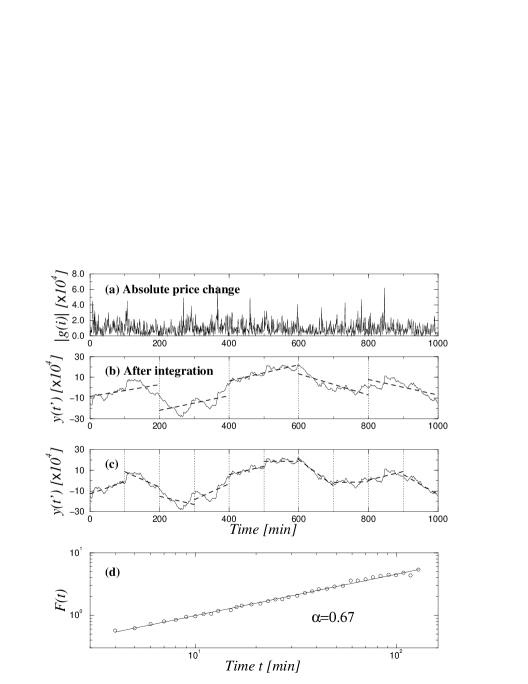
FIG. 13.: Description of DFA method (see text).

REFERENCES

- [1] J.-P. Bouchaud and M. Potters, Theorie des Risques Financieres, (Alea-Saclay, Eyrolles 1998); I. Kondor and J. Kertesz (eds) Econophysics: An Emerging Science (Kluwer, Dordrecht, 1999).
- [2] B. B. Mandelbrot, J. Business 36, 393 (1963).
- [3] R. N. Mantegna, Physica A 179, 232 (1991).
- [4] H. Takayasu, A. H. Sato, and M. Takayasu, Phys. Rev. Lett. 79, 966 (1997); H. Takayasu, H. Miura, T. Hirabayashi and K. Hamada, Physica A 184, 127 (1992); H. Takayasu and K. Okuyama, Fractals 6, 67 (1998).
- [5] M. Marsili and Y.-C. Zhang, Phys. Rev. Lett. 80, 2741 (1998); G. Caldarelli, M. Marsili, and Y.-C. Zhang, Europhys. Lett. 40, 479 (1997); S. Galluccio et al, Physica A 245, 423 (1997).
- [6] N. Vandewalle and M. Ausloos, Int. J. Mod. Phys. C 9, 711 (1998); Eur. Phys. J. B 4, 257 (1998); N. Vandewalle et al, Physica A 255, 201 (1998).
- [7] J.-P. Bouchaud and D. Sornette, J. Phys. I (France) 4, 863 (1994); J.-P. Bouchaud and R. Cont, Eur. Phys. J. B 6, 543 (1998); M. Potters, R. Cont, and J.-P. Bouchaud, Europhys. Lett. 41, 239 (1998).
- [8] A. Johansen and D. Sornette, Int. J. Mod. Phys. C 10 (1999); D. Sornette, A. Johansen, and J.-P. Bouchaud, J. Phys. I (France) 6, 167 (1996); A. Arnoedo, J.-F. Muzy and D. Sornette, Eur. Phys. J. B 2, 277 (1998).
- [9] D. Chowdhury and D. Stauffer, Eur. Phys. J. B (in press); I. Chang and D. Stauffer, Physica A 264, 1 (1999); D. Stauffer and T. J. P. Penna, Physica A 256, 284 (1998); D. Stauffer, P. M. C. de Oliveria and A. T. Bernardes, Int. J. Theor. Appl. Finance (in press).
- [10] T. Lux and M. Marchesi, Nature 297, 498 (1999); T. Lux, J. Econ. Behav. Organizat. 33, 143 (1998); J. Econ. Dyn. Control 22, 1 (1997); Appl. Econ. Lett. 3, 701 (1996).
- [11] M. Levy, H. Levy and S. Solomon, Economics Letters 45, 103 (1994); M. Levy and S. Solomon, Int. J. Mod. Phys C 7, 65 (1996).
- [12] S. Ghashghaie, W. Breymann, J. Peinke, P. Talkner and Y. Dodge, Nature 381, 767 (1996).
- [13] R. N. Mantegna and H. E. Stanley, Nature 376, 46 (1995); R. N. Mantegna and H. E. Stanley, Nature 383, 587 (1996); R. N. Mantegna and H. E. Stanley, Physica A 239, 255 (1997).
- [14] A. Pagan, J. Empirical Finance 3, 15 (1996); and references therein.
- [15] Z. Ding, C. W. J. Granger and R. F. Engle, J. Empirical Finance 1, 83 (1983).
- [16] M. M. Dacorogna, U. A. Muller, R. J. Nagler, R. B. Olsen and O. V. Pictet, J. International Money and Finance 12, 413 (1993).
- [17] T. Bollerslev, R. Y. Chou and K. F. Kroner, J. Econometrics 52, 5 (1992); G. W. Schwert, The Journal of Finance 44, 1115 (1989); A. R. Gallant, P. E. Rossi and G. Tauchen, The Review of Financial Studies 5, 199 (1992); B. Le Baron, Journal of Business 65, 199 (1992); K. Chan, K. C. Chan and G. A. Karolyi The Review of Financial Studies 4, 657 (1991).
- [18] R. Cont, Statistical Finance: Empirical study and theoretical modeling of price variations in financial markets, PhD thesis, Universite de Paris XI, 1998; see also cond-mat/9705075.
- [19] Y. Liu, P. Cizeau, M. Meyer, C.-K. Peng, and H. E. Stanley, Physica A 245, 437 (1997).
- [20] P. Cizeau, Y. Liu, M. Meyer, C.-K. Peng, and H. E. Stanley, Physica A 245, 441 (1997).
- [21] M. Pasquini and M. Serva, cond-mat/9810232.
- [22] P. Bak, K. Chen, J. A. Scheinkman and M. Woodford, Richerche Economichi 47, 3 (1993); J. A. Scheinkman and J. Woodford, American Economic Review 84, 417 (1994). P. Bak, How nature works: the science of self-organized criticality, (New York, NY, 1996).
- [23] P. R. Krugman, The Self-Organizing Economy (Blackwell Publishers, Cambridge, 1996).
- [24] P. Gopikrishnan, M. Meyer, L. A. N. Amaral and H. E. Stanley, Eur. Phys. J. B 3, 139 (1998).
- [25] F. Black and M. Scholes, J. of Political Economy 81, 637 (1973).
- [26] J. Cox, S. Ross and M. Rubinstein, J. of Financial Economics 7, 229 (1979).
- [27] The Trades and Quotes Database, 24 CD-ROM for ’94-’95, published by the New York Stock Exchange.
- [28] P. Gopikrishnan, V. Plerou, M. Meyer, L. A. N. Amaral and H. E. Stanley, to be published.
- [29] The majority of the chosen 500 companies belong to the S&P 500 index. However the companies comprising the S&P 500 index varies by a small fraction every year, but this effect is not considerable for the 2-year period.
- [30] J. Beran, Statistics for Long-Memory Processes (Chapman & Hall, NY, 1994).
- [31] E.-F. Fama, J. Finance 25, 383 (1970).
- [32] R. A. Wood, T. H. McInish and J. K. Ord, J. of Finance 40, 723 (1985).
- [33] L. Harris, J. of Financial Economics 16, 99 (1986).
- [34] A. Admati and P. Pfleiderer, Review of Financial Studies 1, 3 (1988).
- [35] V. Plerou, P. Gopikrishnan, L. A. N. Amaral and H. E. Stanley, to be published.
- [36] P. D. Ekman, The Journal of Futures Markets 12, 365 (1992).
- [37] A. Admati and P. Pfleiderer, Review of Financial Studies 1, 3 (1988).
- [38] C.-K. Peng, S. V. Buldyrev, S. Havlin, M. Simons, H. E. Stanley and A. L. Goldberger, Phys. Rev. E 49, 1684 (1994).
- [39] C.-K. Peng, S. Havlin, H. E. Stanley and A. L. Goldberger, CHAOS 5, 82 (1995).
- [40] N. Iyengar, C.-K. Peng, R. Morin, A. L. Goldberger and L. A. Lipsitz, Am J Physiol 271, R1078 (1997).
- [41] J. M. Hausdorff and C.-K. Peng. Phys Rev E 54, 2154 (1996).
- [42] J. Feder, Fractals, (Plenum Press, New York 1988).
- [43] E. W. Montroll and W. W. Badger, Introduction to Quantitative Aspects of Social Phenomena, (Gordon and Breach Science publishers, New York, 1974).
- [44] A. Bunde and S. Havlin, in Fractals and Disordered Systems, A. Bunde and S. Havlin (editors), ed. (Springer, Heidelberg 1996).
- [45] W. H. Press, Comments Astrophys 7, 103 (1978).