Conformations of Closed DNA

Abstract

We examine the conformations of a model for a short segment of closed DNA. The molecule is represented as a cylindrically symmetric elastic rod with a constraint corresponding to a specification of the linking number. We obtain analytic expressions leading to the spatial configuration of a family of solutions representing distortions that interpolate between the circular form of DNA and a figure-eight form that represents the onset of interwinding. We are also able to generate knotted loops. We suggest ways to use our approach to produce other configurations relevant to studies of DNA structure. The stability of the distorted configurations is assessed, along with the effects of fluctuations on the free energy of the various configurations.

I introduction

If a segment of untwisted rod is forced to close smoothly on itself, it will take on a circular shape in order to minimize the elastic energy. Thermal fluctuations will exert a significant effect on this configuration only if the circumference of the circle is greater than the temperature-dependent persistence length of this segment. When the looped rod is also forced to undergo a twist, the circular shape may prove to be unstable. The rod will then either distort into a non-planar, non-intersecting form, or it may wind about itself, in an interwound, or “plectonemic,” configuration [2, 3, 4, 5, 6, 7, 8].

When torsional and flexing stresses are not too severe, [9] the DNA molecule can be modeled as such a rod. A short enough segment of looped DNA will thus take on shapes determined by the minization of elastic energy. Planar shapes, characteristic of “relaxed” DNA have been observed, as have the plectonemic forms when the molecule is over-or underwound. The distortion, or supercoiling, of DNA under the influence of torsional stresses is widely believed to have significant implications with respect to the action of this molecule in biological settings [10]. That this is so may be inferred from the existence of enzymes known as topoisomerases, which act to facilitate the alteration of the torsional characteristics of DNA configurations [10, 11, 12, 13].

The elastic model of DNA has been the subject of intense research in the past 30 years. Theoretical appraches to this problem include Lagrangian mechanics[14, 15, 16, 17, 18], b-splines and (numerical) molecular dynamics [19], and statistical mechanics[20]. Only recently has it been possible to determine the equilibrium configuration of a closed segment of DNA, as modeled by distorted rod[21]. A comprehensive discussion of the properties of these equilibrium configurations has not yet been published.

In this paper we contribute to the knowledge of this configuration by describing a method by which one can obtain the shape of a closed section of an elastic rod, along with various key properties of this system, including its twist, writhe, linking number and energy. We will use this formalism to generate both unknotted and knotted forms of closed DNA. We will also outline how our formalism can be exploited to produce other shapes of interest to DNA researchers.

The configurations that will be discussed include those that arise as a result of the the supercoiling instability for a closed loop. We will also examine the configurations that represent the evolution of higher energy deformation of a circular loop. In addition, we will briefly discuss configurations that are associated with knotted loops. Such knots include, but are not limited to, the trefoil. All the more elaborate configurations are unstable with respect to fluctuations about the solutions that extremize the energy of the loop. However, it is possible to envision mechanisms, analogous to those leading to the nuclesome structure [10, 22], that stabilize these configurations and, therefore, cause them to be relevant to biological systems.

As noted about, we will discuss the mechanical stability of the configurations to be studied, and will present results with regard to the contribution to the free energy of thermal fluctuations about the minimizing shape. These results will be relevant as long as thermal fluctuations do not give rise to a significantly alteration of the shape that the rod takes, and, as noted above, if the circumference of the rod is not large compared to the rod’s persistence length. The precise criterion for this will be examined later on in this paper.

The most important advance in the work presented here is the algorithm for the generation of various closed structures and the analysis of the stability of the configurations, particularly the one associated with the principal supercoiling instability. On the basis of the stability analysis, it is clear that only some of the configurations that one can generate with the use of the methods described in this paper are, in and of themselves, mechanically stable. However, the existence of devices that support non-interwound supercoiled configurations in the case of open strands of DNA [10, 22] allow one to speculate as to the possible relevance of those configurations to DNA in biological settings. Furthermore, one can envision utilizing these methods in conjunction with other calculational tools to study the mechanical properties and packing configurations of longer strands of DNA.

The paper is organized as follows. First, the mechanical model is described and important parameters are defined. Of especial importance is an identification of the parameters that will be adjusted in order to obtain solutions of the energy extremum equations. Key quantities, including topological invariants, will be defined in terms of those parameters. The stability of the circular configuration of a closed rod under torsional stress is then assessed. The principal instability is identified, and it is shown how to obtain the family of closed curves that represent the evolution of this instability. This family interpolates between the circle and a figure eight, that latter of which lies at the onset of interwinding. The stability of the members of this class is then assessed. It is found that they are, indeed, stable against small fluctuations. Then, it is shown that the method by which the outcome of the supercoiling instability is investigated can be utilized to generate deformed configurations, among which are configurations in which the closed loop is also knotted. Finally, there is a brief discussion of the way in which the contributions of fluctuations about the classical solution configurations. Details and background are relegated to appendices.

II Elastic Model and Expressions of Interest

In previous work we have outlined some developments in the elastic model of DNA[23]. The molecule is represented as a slender cylindrical elastic rod. At each point $s$ the rod is characterized by relating the local coordinate frame ${\cal F}$ to the frame ${\cal F}_{0}$ rigidly embedded in the curve in its relaxed configuration. The relationship between the stressed and unstressed local frames is specified by Euler angles $\theta(s),\phi(s),\psi(s)$ needed to rotate ${\cal F}_{0}$ into $\cal F$.

We begin by summarizing some of the results needed for this paper. We denote the elastic constants of bending and torsional stiffness by $A$ and $C$, respectively. The length of the rod is denoted by $L$. The elastic energy is given by

$$E_{el}=\int_{0}^{L}ds\;\left(\frac{A}{2}\left(\dot{\phi}^{2}\sin^{2}\theta+\dot{\theta}^{2}\right)+\frac{C}{2}\left(\dot{\phi}\cos\theta+\dot{\psi}\right)^{2}\right)$$ (1)

The “dot” notation for derivatives is used interchangeably with the explicit derivative with respect to arc-length, $d/ds$.

The twist is given by

$${\cal T}w=\frac{1}{2\pi}\int_{0}^{L}ds\;\left(\dot{\phi}\cos\theta+\dot{\psi}\right)$$ (2)

A relevant result from our previous work is that ${\cal L}k$, the linking number, can be written as

$${\cal L}k={\cal I}-1+\frac{1}{2\pi}\int_{0}^{L}\left(\dot{\phi}+\dot{\psi}\right)\;ds$$ (3)

Where we have used Fuller’s theorem[24] to obtain the writhe, and White’s theorem[25] for the total link. The quantity ${\cal I}$ is an integer that encodes the knotting of the loop. It is equal to the number of signed crossings of the loop, assuming that it has been flattened out as much as possible.

III Candidates: The Elastic Extrema

A Stability and Excitations of the Circular Loop

As a precursor to the discussion of the possible deformations of a closed loop, we review the family of excitations of a closed, circular loop, and the conditions under which this configurations may become unstable to one or more of these excitations. Detailed discussion of these issues has been relegated to Appendices A and B. The Appendices also contain derivations of key formulas presented below.

The excitation of a circular loop is describable in terms of the deviation of the Euler angle $\theta$ from the constant value of $\pi/2$ that it has in the case of a circle. If we write $\theta(s)=\pi/2+\gamma(s)$, then small excitations about a circular shape will be of the form

$$\gamma(s)\propto\cos\left(\frac{2\pi n}{L}+\delta\right)$$ (4)

where $n$ is an integer (possibly 0) and $\delta$ is an arbitrary phase factor. The energy of such a sinusoidal excitation proportional to

$$E_{n}=\frac{A}{2}\left(\frac{2\pi}{L}\right)^{2}\left\{n^{2}-1-\left(\frac{C}{A}\right)^{2}{\cal L}k^{2}\right\}$$ (5)

The requirement that the fluctuations leave the loop closed and, also, that they not change the linking number of the loop rule out $n=0$ and $n=1$ as possibilities. The allowed deformation with the smallest energy has $n=2$. Substituting this value into Eq. (5), we find for the energy cost of this excitation

$$E_{2}\propto\frac{A}{2}\left(\frac{2\pi}{L}\right)^{2}\left\{3-\left(\frac{C}{A}\right)^{2}{\cal L}k^{2}\right\}$$ (6)

It is clear that this deformation of the circle can give rise to a lowering of the energy. This state of affairs holds if

$${\cal L}k>\frac{A}{C}\sqrt{3}$$ (7)

In fact, the condition in Eq. (7) is just the requirement for the supercoiling instability of the closed loop. Deformations associated with higher values of $n$ lower the energy of the loop when the condition

$${\cal L}k>\frac{A}{C}\sqrt{n^{2}-1}$$ (8)

holds.

It is clear that the instability with the earliest onset, and the one that will prove dynamically “strongest” is the one with threshold as given by (7).

B A Family of Curves

We start by looking for a family of closed solutions to the Euler-Lagrange equations that represent the evolution of the deformation associated with the supercoiling instability, i.e. $n=2$ in Eqs (4) and (5) above. This family of curves can be indexed by the writhe, ${\cal W}r$, of a member, which ranges from ${\cal W}r=0$ for a simple circle to ${\cal W}r=1$ of the other limiting member of the family, a “figure eight.” The actual constraint imposed on the closed curves that are of relevance to this discussion is that the link is fixed at a predetermined value. We shall therefore examine the conditions under which the family of writhing curves can satisfy the imposition of a linking number

C Euler-Lagrange Minimization

Our goal is to extremize elastic energy and keep the curve closed. The functional to consider for closed configurations of DNA is

$${\cal H}=\int_{0}^{L}dE_{el}-F{\bf t}{\bf{\hat{z}}}\>ds$$ (9)

The first term of (9) is clear—the elastic energy must be extremized. The second term enforces the constraint that the curve minimizing the elastic energy also closes upon itself. In general, one expects to introduce Lagrange multipliers controlling the extent of the curve in all directions. However, one can concentrate on the net displacement in only the $z$ direction, because it is always possible to transform to a a reference frame in which the curve is closed in the $XY$ plane. Written explicitly as a function of Euler angles (9) becomes

$${\cal H}=\int_{0}^{L}\;ds\hskip 14.45377pt \frac{A}{2}\left(\dot{\phi}^{2}\sin^{2}\theta+\dot{\theta}^{2}\right)+$$ (10)

$$+ \frac{C}{2}\left(\dot{\phi}\cos\theta+\dot{\psi}\right)^{2}-F\cos\theta$$ (11)

The extrema are found by applying Euler-Lagrange equations to (11). Denoting the conserved quantities as $J_{\phi}\equiv\partial{\cal H}/\partial\dot{\phi}$ and $J_{\psi}\equiv\partial{\cal H}/\partial\dot{\psi}$ we obtain

$$\dot{\phi} = \frac{J_{\phi}-J_{\psi}\cos\theta}{A\sin\theta}$$ (12)

$$\dot{\psi} = \frac{J_{\psi}}{C}-\dot{\phi}\cos\theta$$ (13)

The equation for $\theta$ is a quadrature obtained by integrating $\partial{\cal H}/\partial\theta=d/ds\partial{\cal H}/\partial\dot{\theta}$ with $E_{0}$ as the constant of integration. Defining $u\equiv\cos\theta$ we see that the behavior of solutions is governed by a cubic polynomial in $u$:

$${\dot{u}}^{2} = \frac{2\left(1-u^{2}\right)}{A}\left(E_{0}-Fu\right)-\frac{1}{A^{2}}\left(J_{\phi}^{2}+J_{\psi}^{2}-2J_{\phi}J_{\psi}u\right)$$ (14)

$$\equiv \frac{2F}{A}\left(u-a\right)\left(u-b\right)\left(u-c\right)$$ (15)

where we order the roots $c\leq u(\equiv\cos\theta(s))\leq b\leq a$. Eq. (15) requires that $\cos\theta(s)$ oscillates between $c$ and $b$. For the distortions studied here, there are two complete ocillations as the the closed curve is traversed once. All the relevant quantities, including the shape of the curve, can be obtained using (15). For example:

$$\phi(s) = \int_{u(s=0)}^{u(s)}\frac{d\phi}{ds}\frac{ds}{du}du\;\;\;\mbox{ with }$$ (16)

$$\frac{ds}{du} = \sqrt{\frac{A}{2F}}\frac{1}{\sqrt{\left(u-a\right)\left(u-b\right)\left(u-c\right)}}$$ (17)

The key to the solution of the equation for the distorted closed loop is the determination of the parameters $F$, $a$, $b$ and $c$.

D Constraints

To complete the analysis we must determine the parameters generated by the minimization procedure. One choice of parameters is the set of invariants $J_{\phi}$ and $J_{\psi}$, the constant $E_{0}$, and the Lagrange multiplier $F$. However, as indicated above, a better practical choice is the Lagrange multiplier $F$ and the parameters $a$, $b$ and $c$. To determine the parameters we impose constraints on the curve. Figure 1 is a good visual guide to the geometric meaning of the constraints. They are

1. The loop closes on itself in the $z$-direction. Because the curve consists of four segments, in each of which the variable $u(s)$ goes from $b$ to $c$, or from $c$ to $b$, we have

   $$\int_{0}^{L/4}u(s)ds=0$$ (18)

2. The loop goes through one quarter of a turn in each segment. This reduces to

   $$\int_{0}^{L/4}\frac{d\phi(s)}{ds}ds=\frac{\pi}{2}$$ (19)

3. The linking number takes on a predetermined value for the loop. This requirement leads to the following mathematical constraint on the solution to the Euler Lagrange equations.

   $$\int_{0}^{L}\frac{d\psi(s)}{ds}ds={\cal L}k$$ (20)

4. Finally, the length of the loop takes on a predetermined value. Mathematically,

   $$\int_{0}^{L}ds=L$$ (21)

   The above condition is not as tautological as it seems. The actual parameterization of the curve will be in terms of the dependence of quantities on the cosine of the Euler angle $\theta(s)$.

E Reparameterization

At this point we reparameterize the problem in terms of $F,a,b,c$ instead of $F,E_{0},J_{\phi},J_{\psi}$. Parametrizing the problem by the roots of the polynomial is extremely advantageous: it makes the analytic manipulations more transparent; it also streamlines the computational tasks. The two sets of parameters are related in the following manner:

$$E_{0} = F\left(a+b+c\right))$$ (22)

$$J_{\phi} = \sqrt{\frac{AF}{2}}\left(p_{1}\pm p_{2}\right);\;\;\;J_{\psi}=\sqrt{\frac{AF}{2}}\left(p_{1}\mp p_{2}\right)$$ (23)

with $$\;p_{1\choose 2}\equiv\left[(c\pm 1)(b\pm 1)(a\pm 1)\right]^{1/2}$$ (24)

The choice of branch ($\pm$) is imposed by the family of configurations sought. For circular DNA without intrinsic curvature, $J_{\phi}$ takes a $-$, and $J_{\psi}$ correspondingly a $+$. Let us make some definitions that render the notation more transparent:

$$\Delta b\equiv\left(b-c\right)\;\;;\;\;\Delta a\equiv\left(a-c\right)$$ (25)

$$q\equiv\sqrt{\frac{\Delta b}{\Delta a}}$$ (26)

Employing (17) we rewrite the constraint equations, (18), (19), and (21), in terms of the new parameters:

$$aK\left(q\right)=\Delta aE\left(q\right)$$ (27)

$$\pi/2\;\;=\;\;\frac{1}{\Delta a}\left[\left|\frac{(a+1)(b+1)}{(c+1)}\right|^{1/2}\Pi\left(\frac{\Delta b}{-1-c},q\right)\right.-$$ (28)

$$\hskip 61.17325pt-\left.\left|\frac{(a-1)(b-1)}{(c-1)}\right|^{1/2}\Pi\left(\frac{\Delta b}{1-c},q\right)\right]$$ (29)

$$F=\frac{32A}{\Delta aL^{2}}K\left(q\right)\;\;\;\;$$ (30)

Where $K,E\mbox{ and }\Pi$ are complete elliptic integrals of the first, second and third kind, respectively. The issue of the constraint on linking number will be left for later discussion.

F Solving for $a$, $b$, $c$ and $F$

We find that the optimal procedure for calculation of parameters appropriate to a solution is to utilize (30) to eliminate $F$, then (27) and (29) eliminate $\Delta a$ and $c$. Because the writhe, ${\cal W}r$, is a monotonically increasing function of $\Delta b$, we make use of this property to classify distinguish between the members of a family of curves. Once the constants $F,a,b,c$ are determined, the desired solutions and all the relevant quantities are computed via elliptic integrals. For example, the explicit expression for $\theta(s)$ in the first quarter of oscillation is (we have inverted (17)):

$$\cos\theta=\Delta b\mbox{ sn}^{2}\left(\sqrt{\frac{F\Delta c}{2A}}s,\sqrt{\frac{\Delta b}{\Delta a}}\right)-c$$ (31)

$\phi\mbox{ and }\psi$ are obtained similarly from (12) and (13).

Figure 2 displays the family of curves computed in the manner discussed above. Since the constraint equations involve elliptic integrals, finding a solution on a computer is virtually instanteneous; analytically and computationally elliptic integrals are equivalent to, say, $\arcsin$.

G Bounding Members: Circle and Figure Eight

Let us check whether the initial member of our family, a circle with ${\cal W}r=0$ joins smoothly with the previously known stable family of twisted circles[26]. The circle corresponds to ${\cal W}r=0$. A circle in the $XY$ plane the curve must have $b_{0}=c_{0}=0$. (29) now states that

$$\frac{1}{\sqrt{a}_{0}}\left(\sqrt{a_{0}+1}-\sqrt{a_{0}-1}\right)=1$$ (32)

which in turn gives (33)

$${J_{\psi}}_{0}=\frac{2\pi A}{L}\frac{1}{\sqrt{a}_{0}}\left(\sqrt{a_{0}+1}+\sqrt{a_{0}-1}\right)=\frac{2\pi A}{L}\sqrt{3}$$ (34)

Combining (2) and (13) to obtain the twist, ${\cal T}w$, of the circle (34) gives

$${\cal T}w_{0}=\frac{L}{2\pi}{J_{\psi}}_{0}=\sqrt{3}\frac{A}{C}$$ (35)

It is also of interest to compute the ${\cal T}w$ of the figure eight, which, like the circle, can be performed virtually by inspection. The figure lies in the $YZ$ plane, which forces $\phi$ to behave as follows: (refer to Figure 1 for visualization)

$${\dot{\phi}}_{8}=\pi\left(\delta\left(0\right)+\delta\left(\frac{L}{2}\right)\right)$$ (36)

Combining (36) and (12) forces ${J_{\phi}}_{8}={J_{\psi}}_{8}=0$ which immediately sets ${\cal T}w_{8}=0$. The value of $\Delta b_{8}$ is easily determined from the fact that $c_{8}=-1$ (this can be seen from the curve itself) necessitating $a=1$. Then (29) yields $\Delta b_{8}=1.6522\ldots$.

IV Linking Number and the Plectonemic Transition

We have found a family of writhing solutions that are the extrema of elastic energy. The writhe of the curves covers the range $0\leq{\cal W}r\leq 1$. However, the physical constraint imposed on the molecule is ${\cal L}k$, the linking number. The explicit expressions for ${\cal T}w$, ${\cal L}k$ and ${\cal W}r$ are easily obtained:

$${\cal T}w = \frac{2\pi}{\sqrt{\Delta a}}K\left(q\right)\left(p_{1}+p_{2}\right)\frac{A}{C}$$ (37)

$${\cal W}r = \frac{2\pi}{\sqrt{\Delta a}}\left[-K\left(q\right)\left(p_{1}+p_{2}\right)\right.$$ (38)

$$+ \left.\frac{p_{1}}{1+c}\Pi\left(\frac{\Delta b}{-1-c},q\right)+\frac{p_{2}}{1-c}\Pi\left(\frac{\Delta b}{1-c},q\right)\right]$$ (39)

and, using White’s theorem[25]

$${\cal L}k={\cal T}w+{\cal W}r$$ (40)

With reference to Figure 3, we can now describe what happens to a deformed loop of DNA as the linking number is increased. The loop remains a circle until $\Delta{\cal L}k=\sqrt{3}A/C$. After that there are three possibilities. If $A/C\leq 0.5$ then the writhing family supports a steady increase to the linking number limit ${\cal L}k=1$ of the figure eight and the molecule folds continuously until self-crossing occurs. Further increase of ${\cal L}k$ presumably results in a plectonemic configuration. If $0.5\leq A/C\leq 1$ the one can expect the curve to distort continuously until the writhe achieves some value intermediate between zero and one. There is, at this threshold value of the writhe, a transition, almost certainly to an interwound form. When $A/C>1$, none of the members of the writhing family support the neccesary linking number, and as soon as $\Delta{\cal L}k$ exceeds the supercoiling threshold value $\sqrt{3}A/C$ the twisted circle snaps into a plectoneme. An interesting fact is that this behavior is independent of the length of the molecule. That this ought to be so follows from the absence of an absolute length scale in the problem of the deformed loop.

Greater insight into the behavior of the deforming loop is gained if one also investigates the way in which the energy depends on the various properties of the loop. The energy can be expressed in terms of the previously introduced quantities. A straightforward calculation yields for the energy of the loop

$$E=F\left\{\left(a+b+c\right)+\frac{1}{4}\left(p_{1}+p_{2}\right)^{2}\left[\frac{A}{C}-1\right]\right\}\int ds$$ (41)

Where the final integral is over arclength. Expressing the circumference of the loop in terms of $F$, $a$, $b$ and $c$, we obtain the following result for the energy in terms of the total circumference of the loop, $l$, the bending modulus, $A$, and the parmeters $a$, $b$, and $c$:

$$E=\frac{2A}{l}\left\{\left(a+b+c\right)+\frac{1}{4}\left(p_{1}+p_{2}\right)^{2}\left[\frac{A}{C}-1\right]\right\}\left(\int_{c}^{b}\frac{du}{\sqrt{(a-u)(b-u)(u-c)}}\right)^{2}$$ (42)

The energy of the loops as a function of writhe for various values of the modulus ratio $A/C$ is plotted in Figure 4. A few facts about the energies of the deformed configuration can be established numerically (and we do not doubt that analytic demonstrations can also be constructed). First, the energy is a monotonically increasing function of linking number, if not of writhe. This is not immediately evident in Figure 4, although it is indicated, in that the energy increases or decreases monotonically with writhe when the link does so. Furthermore, when there is a maximum in link as a function of writhe, there is also an energy maximum, and, as indicated in Figures 3 and 4, the maxima occur at the same value of the writhe.

In addition, when there is a maximum in the linking number as the writhe increases from zero to one, so that there are two possible writhes associated with the same linking number in for a range of the latter quantity, the configuration with the lower writhe always has the lower energy. This can be established by a separate set of calculations. This implies that when, for instance, $0.5<A/C<1$, the loop, in distorting from its planar form, will not be susceptible to a discontinuous distortion to a more highly writhed, but not interwound, configuration before it “snaps” to a plectoneme. In the absence of thermal fluctuations or external perturbations, that transition will to occur when the link has reached its maximum value as a function of writhe.

For a more detailed discussion of the energetics of the deforming loop, along with a calcuation of the energy of the plectoneme, the reader is referred to [21]

V Stability of the deformed loop

Given the existence of the solutions for the deformed loop corresponding to the evolution of the supercoiling instability, it is desirable to determine whether these solutions are, themselves, stable against small fluctuations. There is no a priori guarantee that this is so. We will find, in fact, that the stability of the closed configuration is enforced by the relatively large number of constraints that must be satisfied by fluctuations about the extremizing solutions to the Euler-Lagrange equations. A number of technical details associated with the determination of the stability of a configuration are to be found in various appendices.

A Stability in the Absence of Constraints: the Translation Mode

The energy of a fluctuation about a solution to the Euler-Lagrange equation is expressible in terms of solutions to the linear second order differential equation (A14), equivalent to the Schrödinger equation of a particle in the potential (LABEL:potential1). In particular, any fluctuation, $\zeta(s)$ of the Euler angle $\theta(s)$ about the form it takes in an extremizing solution can be written in the form

$$\zeta(s)=\sum_{l}K_{l}\Psi_{l}(s)$$ (43)

where $\Psi_{l}(s)$ is a solution to Eq. (A14), with eigenvalue $\lambda_{l}$. Assuming that the $\Psi_{l}$’s are normalized, the energy of this fluctuation is given by

$$\sum_{l}K_{l}^{2}\lambda_{l}$$ (44)

The extremizing solution will be stable as long as there are no solutions to Eq. (A14) with negative eigenvalues. Now, consider the potential $V(s)$, displayed in Figure 5, associated with one particular member of the family of solutions that we have been considering.

A striking property of this potential is that it is always negative. From this one can infer that there are solutions of the Schrödinger-like equation with negative eigenvalues. In fact, the existence of such states is guaranteed by the existence of the translational mode—the “fluctuation” equal to the derivative with respect to arc length of the extremizing $\theta(s)$. As the system is invariant with respect to translations along the closed loop, the infinitesimal transformation of the extremizing solution $\theta_{cl}(s)\rightarrow\theta_{cl}(s+\delta s)=\theta_{cl}(s)+\delta sd\theta_{cl}(s)/ds$ has no effect on the energy of the configuration. The function $\Phi_{t}(s)\propto d\theta_{cl}(s)/ds$ has the requisite periodicity, in that it is unchanged if $s$ goes to $s\pm nL$. This implies the existence of a solution to the Schrödinger equation with zero eigenvalue. This solution is displayed in Figure 6. In both Figure 5 and 6, the arclength parameter ranges from $-L/2$ to $L/2$. This will prove to be useful later on, when we take advantage of the reflection invariance of the portential $V(s)$.

The important thing to note is that the translational mode has nodes. Note, furthermore, that this mode is odd on reflection about $s=0$. On the basis of a simple node-counting argument, one can readily establish that there will be another antisymmetric solution to the equation (A14), having fewer nodes in the interval $-L/2<s<L/2$, and, hence, a lower eigenvalue than the translational mode. This lower eigenvalue is necessarily negative. As it turns out, there are two symmetric solutions to (A14) having the requisite periodicity and negative $\lambda$’s. The extremizing solution is, thus, nominally unstable with respect to three kinds of fluctuations.

B Effects of Constraints

Certain constraints apply to any fluctuation in a closed loop. In fact, there are five such constraints, listed in Appendix A. These constraints must be incorporated into any calculation of the stability of an extremizing solution. The general effect of such constraints on the stability calculation is outlined in Appendix C. The determination of the stability of a deformed loop amounts to a search for zeros of a determinant obtained by sandwiching a response kernel between five different functions, each associated with one of the five constraints that must be satisfied by any small variation of the solution to the Euler Lagrange equations for the extremal loop configuration. The five functions are readily extracted from the integrals in Eqs. (A23)–(A29). With the use of symmetry arguments, one can verify that the five-by-five matrix constructed out of the response kernel, which is exhibited in Appendix D, reduces to a four-by-for matrix and a one-by-one matrix. The latter matrix consists of the expectation value of the response kernel with respect to the function associated with closure in the $y$ direction. This function is contained in the integral in Eq. (A27).

The matrices are straightforwardly constructed, although the calculation is somewhat tedious. We find that all the configurations associated with the supercoiling instability that interpolate between the circle and the figure eight are mechanically stable in that the for no negative value of the parameter $\lambda$ does the determinant pass through zero. An example of the calculation of this determinant for a particular deformation of the circular loop is displayed in Figures 7, 8 and 9.

VI Generalizations

A Higher Order Deformations

The solution that interpolates between the supercoiling instability and the figure eight deformation bordering on the regime in which the loop interwinds does not represent the only possibility for deformation. One can also generate deformed loops associated with the evolution of higher energy excitations of the circular loop. This is accomplished by altering the requirement on the change in the Euler angle $\phi$ over a complete “period” of the oscillation of the variable $u(s)=\cos\theta(s)$, as it cycles between its limiting values of $b$ and $c$. If, instead of asking that $\phi$ advance by $\pi/2$ in half a period, one requires a change of $\pi/n$, then it is possible to generate a family of solutions to the Euler-Lagrange equations associated with the excitations having $n$ periods around the circumference of the circular loop. Figure 10 displays such a distortion of the circular loop. Here, $n=5$. The stability analysis of this this family of solutions is straightforward. Starting with the translational mode, one counts nodes and determines the number of solutions to the eigenvalue equation for fluctuations for which $\lambda$ must be negative. There are simply too many to allow for stabilization by the action of constraints. In the absence of external stabilizing mechanisms, such as histones or their equivalent, a loop will spontaneously distort out of this configuration.

B Knotted Configurations

It is possible to generate solutions to the Euler Lagrange equations for the extremization of the elastic energy that close and that are, in addition, knotted. Again, one simply alters the requirement on the way in which the Euler angle $\phi$ advances over the course of a “period” in the oscillation of the quantity $u(s)=\cos\theta(s)$ between its two limiting values of $b$ and $c$. Imposing the requirement that the change in $\phi(s)$ is equal to $m\pi/n$, where $m$ and $n$ are relatively prime, and $m<n$, one obtains knotted solutions. For example, setting $n=3$ and $m=2$, one generates closed loops in the form of trefoils. An example of this solution to the Euler-Lagrange equations is displayed in Figure 11. Alternatively, setting $n=5$ and $m=3$, one obtains a knotted solution with fivefold symmetry. This solution is shown in Figure 12. Both displayed loops are members of a family having the same topological characteristics. These closed extremal curves interpolate between nearly circular, “braided” loops and relatively strongly writhing forms, such as are displayed in the figures.

It is possible to assess the stability of the solutions shown in the figure. In this case the constraints on fluctuations do not suffice to stabilize them against deformations that lower their elastic energy. Thus, in the absence of externally imposed stabilizing mechanisms, these extremal configurations are not mechanically stable.

The trefoil solution has also been generated in finite element calculations [19], and knotted configurations of closed DNA have long been known to exist in vivo [32]

VII Entropic Corrections

The analysis of the fluctuations about the classical solution described abve readily lends itself to a calculation of the entropic contributions to the partition function of a loop of DNA at finite temperature. Performing an expansion of the Euler angles about the form taken in a solution to the Euler Lagrange equation and retaining terms that are second order in the deviation of those angles about their classical values, one obtains the following expression for the partition function of a closed DNA segment

$$Z\propto e^{-\beta E_{el}\left(\theta_{0},\phi_{0},\psi_{0}\right)}\int{\cal D}\gamma(s)\exp\left[-\beta\langle\gamma(s)|{\cal L}|\gamma(s)\rangle\right]$$ (45)

where the operator ${\cal L}$ is given by

$${\cal L}=-\frac{d^{2}}{ds^{2}}+V(s)$$ (46)

with $V(s)$ as defined in Eq. (LABEL:potential1). The quantity $\gamma(s)$ is the deviation of the Euler angle $\theta(s)$ from its classical value.

The integral over $\gamma(s)$ in Eq. (45) yields the inverse square root of the Fredholm determinant, $F(0)$, of the operator ${\cal L}$, where

$$F(\lambda)=\prod_{l}\left(\lambda_{l}-\lambda\right)$$ (47)

The quantities $\lambda_{l}$ are the eigenvalues of the operator ${\cal L}$. The Fredholm determinant is readily calculated with the use of a method commonly exploited in the study of instanton effects in nonlinear systems [33]. The application of this method to the case at hand is outlined in Appendix E. One finds that the determinant can be expressed in terms of the quantity $T(\lambda)$, defined in Eq. (E9). This quantity is plotted for a characteristic member of family of deformed loops that interpolate between a circle and a figure eight in Figures 13 and 14. A noteworthy property of the Fredholm determinant as displayed in the plots is the fact that this function of $\lambda$ possesses a zero at $\lambda=0$—this as a consequence of the existence of the translation mode—and the fact that there are zeros at negative values of $\lambda$. These latter features point to the instability of the unconstrained solution to the Euler-Lagrange equations.

Given that $T(0)$, and, by extension, $F(0)$, is equal to zero, one expect the gaussian integration over the variable $\gamma(s)$ to blow up. However, the translational mode has a well-defined influence on the fluctuation spectrum. It simply gives rise to a multiplicative factor reflecting the freedom one has in the fixing location the distortion on the loop. One eliminates this zero from the Fredholm determinant by noting that

$$\left.\frac{d}{d\lambda}\prod_{l}\left(\lambda_{l}-\lambda\right)\right|_{\lambda-\lambda_{l_{0}}}=-\prod_{l\neq l_{0}}\left(\lambda_{l}-\lambda_{l_{0}}\right)$$ (48)

This means that we can eliminate the translational mode from the Fredholm determinant by making the replacement

$$T(0)\rightarrow-\left.\frac{dT(\lambda)}{d\lambda}\right|_{\lambda=0}\equiv-T^{\prime}(0)$$ (49)

The result of an unconstrained gaussian integration over fluctuations is, then, proportional to

$$\beta^{-N/2}\left(-T^{\prime}(0)\right)^{-1/2}$$ (50)

where $N$ is equal to the number of modes contributing to the fluctuation spectrum. In light of the behavior of $T(\lambda)$, as displayed in Figures 13 and 14, this result is clearly pathological.

A Constraints

Of course, one is not allowed to integrate freely over all fluctuations. The constraints on the influence of those fluctuations are the same as applied in the linear stability analysis. The imposition of constraints leads to an additional multiplicative term

$$\left(\det\left(G\left(\lambda=0\right)\right)\right)^{-1/2}$$ (51)

For the generaly principle underlying this result, see Appendix F. The matrix $G$ is a $5\times 5$ version of the matrix introduced in Appendix C. The determinant of this matrix has poles at the negative values of $\lambda$ at which the function $T(\lambda)$ passes through zero. Figures 7, 8 and 9 display the dependence on $\lambda$ of the two quantities that when multiplied together yield this determinant. The plots in these figures are for the same solution to the Euler-Lagrange equation as generated the $T(\lambda)$ displayed in Figures 13 and 14. The quantity

$$\beta^{-N/2}\left(-T^{\prime}(0)\det\left(G\left(\lambda=0\right)\right)\right)^{-1/2}$$ (52)

represents the contributions of fluctuations about the classical solution, to within readily calcuated numerical factors. In the example for which quantities are displayed, the argument of the square root is finite and positive.

VIII Conclusion

We have presented a formalism for obtaining the elastic mimima of a segment of closed DNA subject to a constraint in the linking number. The methods exploited here have been utilized to construct the family of deformations interpolating between the “relaxed” circular form taken by such a segment when the molecule is insufficiently under- or overwound to induce a supercoiling transition and the figure eight form that represents the threshold of interwinding. The members of this family are stable with respect to small fluctuations. The same methods also give rise to solutions that represent the evolution of “higher order” fluctuations about a circle of the twisted loop. These solutions to the Euler-Lagrange equations for the extremization of the elastic energy of a closed loop are unstable with respect to small fluctuations, in that there exist one or more fluctuation modes that lead to a lowering of the energy with respect to the classical solution. It is also possible to construct knotted solutions to the Euler-Lagrange equations. These configurations also represent saddle-point solutions to the extremization equation. However, as previously noted, it is possible to envision stabilizing mechanisms consistent with the known structure of biological sysems.

In this paper, entire closed loops were generated and studied. The same method can, in principle also be utilized to construct a truly “finite” finite-element-analysis in which elastic models can be traced out with the use of non-infinitesimal segments. Given our experience in the project described herein, we are confident that the properties of the segments can be controlled and explicitly displayed. This ought to give rise to a substantial savings in time and effort in numerical studies of DNA structure.

A Stability considerations

Starting with the expression for the elastic energy

$$E_{el}=\int ds{\cal E}_{el}(s)$$ (A1)

where

$${\cal E}_{el}(s)=\frac{A}{2}\left[\left(\frac{d\theta(s)}{ds}\right)^{2}+\sin^{2}\theta(s)\left(\frac{d\phi(s)}{ds}\right)^{2}\right]+\frac{C}{2}\left[\frac{d\psi(s)}{ds}+\cos\theta(s)\frac{d\phi(s)}{ds}\right]^{2}$$ (A2)

See Eq. (1). We expand the Euler angles about their extremizing values as follows

$$\phi(s) = \phi_{cl}(s)+\alpha(s)$$ (A3)

$$\psi(s) = \psi_{cl}(s)+\beta(s)$$ (A4)

$$\theta(s) = \theta_{cl}(s)+\gamma(s)$$ (A5)

The subscript $cl$ stands for the extremizing, or “classical” values of the Euler angles. The deviations from these classical values, $\alpha(s)$, $\beta(s)$ and $\gamma(s)$, are assumed to be small. Substituting from Eqs. (A3) - (A5) into (A2), one finds at quadratic order in the deviations from the extremizing solutions a local energy equal to

$$\frac{A}{2}\left[\dot{\gamma}(s)^{2}+\dot{\phi}_{cl}(s)^{2}\gamma(s)^{2}\left[\cos^{2}\theta_{cl}(s)-\sin^{2}\theta_{cl}(s)\right]\right.$$ (A6)

$$\left.+4\dot{\alpha}(s)\gamma(s)\dot{\phi}_{cl}\sin\theta_{cl}(s)\cos\theta_{cl}(s)+\dot{\alpha}^{2}\sin^{2}\theta_{cl}(s)\right]$$ (A7)

$$+\frac{C}{2}\left[\left[\dot{\beta}(s)+\dot{\alpha}(s)\cos\theta_{cl}(s)-\dot{\phi}_{cl}(s)\gamma(s)\sin\theta_{cl}(s)\right]^{2}\right.$$ (A8)

$$\left.-2\left[\dot{\psi}_{cl}(s)+\dot{\phi}_{cl}(s)\right]\left[\dot{\alpha}(s)\gamma(s)\sin\theta_{cl}(s)+\dot{\phi}(s)\gamma^{2}(s)\cos\theta_{cl}(s)/2\right]\right]$$ (A9)

When it does not lead to confusion, the, the subscripts will be dropped from the “classical,” or extremum, Euler angles. Because the classical Euler angles satisfy an extremum equation, there is no term linear in the deviations.

A cursory investigation Eq. (A9) reveals that the second-order energy depends on $\alpha(s)$ and $\beta(s)$ only through their derivatives. Minimizing the energy with respect to these variables, we are left with the following dependence of the “fluctuation” energy on the angular variable $\gamma(s)$

$$\frac{A}{2}\left(\frac{d\gamma(s)}{ds}\right)^{2}-\frac{\gamma(s)^{2}}{2}\frac{\left(J_{\phi}^{2}+J_{\psi}^{2}\right)\left(2\cos^{2}\theta(s)+1\right)-J_{\phi}J_{\psi}\cos\theta\left(\cos^{2}\theta+5\right)}{A\sin^{4}\theta}$$ (A10)

Recall that the Euler angle $\theta(s)$ in Eq. (A10) is the solution to the minimzation equation.

The equation (A10) for the energy of a fluctuation can be further reduced if one makes use of the relationship between the quantities $J_{\phi}$ and $J_{\psi}$ and the roots $a$, $b$, and $c$ of the cubic polynomial in Eq. (23). The new form of the energy is

$$\frac{1}{2}\left(\frac{d\gamma(s)}{ds}\right)^{2}$$ (A11)

$$- \frac{1}{4}\frac{\left(2-u(s)\right)\left(1-u(s)\right)^{2}(a+1)(b+1)(c+1)+\left(2+u(s)\right)\left(1+u(s)\right)^{2}(a-1)(1-b)(1-c)}{\left(1-u(s)^{2}\right)^{2}}\gamma(s)^{2}$$ (A12)

The quantity $u(s)$ satisfies Eq. (15). This equation is equivalent to the expectation value of the energy of a particle in a one-dimensional potential. This expectation value can be expressed in terms of the eigensolutions and eigenvalues of the corresponding Schrödinger equation. The stationary version of the Schrödinger equation has the form

$$-\frac{d^{2}\Psi(s)}{ds^{2}}+V(s)\Psi(s)=\lambda\Psi(s)$$ (A14)

where

$$V(s)=$$ (A16)

$$\frac{1}{2}\frac{\left(2-u(s)\right)\left(1-u(s)\right)^{2}(a+1)(b+1)(c+1)+\left(2+u(s)\right)\left(1+u(s)\right)^{2}(a-1)(1-b)(1-c)}{\left(1-u(s)^{2}\right)^{2}}$$

The stability of a fluctuation is tied to the sign of the eigenvalues of the stationary Schrödinger equation. If all the allowed values of $\lambda$ are positive, the solution about which fluctuations occur is positive. On the other hand if there is one or more negative $\lambda$, then an instability exists.

1 Constraints

Fluctuations about the classical solution must obey certain constraints. In particular, they cannot change the following properties of the loop:

1. The loop closes smoothly:

   $$\int_{0}^{L}\frac{d\phi(s)}{ds}ds=2\pi n$$ (A18)

   where $n$ is an integer

2. The net linking number is fixed:

   $$\int_{0}^{L}\frac{d\psi(s)}{ds}ds=\mbox{const.}$$ (A19)

3. The loop closes in the $x$ direction:

   $$\int_{0}^{L}\sin\theta(s)\cos\phi(s)ds=0$$ (A20)

4. The loop closes in the $y$ direction:

   $$\int_{0}^{L}\sin\theta(s)\sin\phi(s)ds=0$$ (A21)

5. The loop closes in the $z$ direction:

   $$\int_{0}^{L}\cos\theta(s)ds=0$$ (A22)

In the above expressions, the Euler angles are not necessarily equal to their extremum values.

Expanding the solution about its extremum form and expressing the fluctuations in the Euler angles $\phi$ and $\psi$ in terms of the fluctuation, $\gamma(s)$, in the Euler angle $\theta(s)$, the conditions above take the forms shown below

1. Smooth closure:

   $$\sqrt{\frac{F}{2A}}\int_{0}^{L}\frac{p_{1}\left(u(s)-1\right)^{2}+p_{2}\left(u(s)+1\right)^{2}}{\left(1-u(s)\right)^{3/2}}\gamma(s)\,ds=0$$ (A23)

   Here, and below, the quantity $u(s)$ is $\cos\theta(s)$, where $\theta(s)$ is the solution to the extremum equations.

2. Constancy of the link:

   $$\sqrt{\frac{F}{2A}}\int_{0}^{L}\frac{p_{1}\left(1-u(s)\right)^{2}-p_{2}\left(1+u(s)\right)^{2}}{\left(1-u(s)^{2}\right)^{3/2}}\gamma(s)\,ds=0$$ (A24)

3. Closure in the $x$ direction:

   $$\int_{0}^{L}\left\{u(s)\cos\phi_{cl}(s)+\sqrt{\frac{F}{2A}}\frac{p_{1}\left(1-u(s)\right)^{2}+p_{2}\left(1+u(s)\right)^{2}}{\left(1-u(s)^{2}\right)^{3/2}}{\cal I}_{x}(s)\right\}\gamma(s)\,ds=0$$ (A25)

   Here, the quantity ${\cal I}_{x}(s)$ is given by

   $${\cal I}_{x}(s)=\int_{L/2}^{s}\sqrt{1-u(s^{\prime})^{2}}\sin\phi_{cl}(s^{\prime})\,ds^{\prime}$$ (A26)

4. Closure in the $y$ direction:

   $$\int_{0}^{L}\left\{u(s)\sin\phi_{cl}(s)-\sqrt{\frac{F}{2A}}\frac{p_{1}\left(1-u(s)\right)^{2}+p_{2}\left(1+u(s)\right)^{2}}{\left(1-u(s)^{2}\right)^{3/2}}{\cal I}_{y}(s)\right\}\gamma(s)\,ds=0$$ (A27)

   where

   $${\cal I}_{y}(s)=\int_{L/2}^{s}\sqrt{1-u(s^{\prime})^{2}}\cos\phi_{cl}(s^{\prime})\,ds^{\prime}$$ (A28)

5. Closure in the $z$ direction:

   $$\int_{0}^{L}\sqrt{1-u(s)^{2}}\gamma(s)\,ds=0$$ (A29)

B Stability analysis of the circular loop

The solution of the extremum equations leading to a circular loop is

$$u(s) = 0$$ (B1)

$$\phi_{cl}(s) = \frac{2\pi s}{L}$$ (B2)

$$\psi_{cl}(s) = {\cal L}k\frac{2\pi s}{L}$$ (B3)

the quantity ${\cal L}k$ being the linking number of the circular loop. Making use of Eq. (A10), we find for the eigenvalue equation for fluctuations

$$\frac{A}{2}\left\{-\frac{d^{2}\gamma(s)}{ds^{2}}-\left[\left(\frac{d\phi_{cl}(s)}{ds}\right)^{2}-\left(\frac{C}{A}\right)^{2}\left(\frac{d\psi_{cl}(s)}{ds}\right)^{2}\right]\gamma(s)\right\}=\lambda\gamma(s)$$ (B4)

substituting for the rate of change of the classical Euler angles, $\phi_{cl}(s)$ and $\phi_{cl}(s)$, the eigenvalue equation becomes

$$\frac{A}{2}\left\{-\frac{d^{2}\gamma(s)}{ds^{2}}-\left(\frac{2\pi}{L}\right)^{2}\left[1+\left(\frac{C}{A}\right)^{2}{\cal L}k^{2}\right]\right\}\gamma(s)=\lambda\gamma(s)$$ (B5)

Now, the solutions to the equation above are

$$\gamma(s)\propto\cos\left(\frac{2\pi n}{L}s+\delta\right)$$ (B6)

where $n$ is an integer and $\delta$ is an arbitrary phase angle. Looking at Eq. (B5), one might be tempted to conclude that the circular loop is always unstable, in that solutions of the form (B6) with $n=0$ and $n=1$ give rise to negative eigenvalues. However, those solutions are inconsistent with the constraints on fluctuations. A cursory inspection of the constraints listed in Eqs. (A23) to (18) reveals that the following conditions must hold in the case of the circular loop

$$\int_{0}^{L}\gamma(s)\,ds = 0$$ (B7)

$$\int_{0}^{L}\gamma(s)\cos\left(\frac{2\pi s}{L}\right)ds = 0$$ (B8)

$$\int_{0}^{L}\gamma(s)\sin\left(\frac{2\pi s}{L}\right)ds = 0$$ (B9)

These three constraints on explicitly rule out flucutations of the form (B6) with $n=0$ or $n=1$. All other values of $n$ are allowed. If we substitute a fluctuation given by (B6) with $n\geq 2$, the equation for the eigenvalue $\lambda$ is

$$\lambda=\frac{A}{2}\left(\frac{2\pi}{L}\right)^{2}\left[n^{2}-1-\left(\frac{C}{A}\right)^{2}{\cal L}k^{2}\right]$$ (B10)

The lowest value of $\lambda$ is associated with the smallest allowed value of $n^{2}$, corresponding to $n=2$. Replacing $n$ by 2 in Eq. (B10), we find

$$\lambda=\frac{A}{2}\left(\frac{2\pi}{L}\right)^{2}\left[3-\left(\frac{C}{A}\right)^{2}{\cal L}k^{2}\right]$$ (B11)

According to Eq. (B11), $\lambda$ will be negative, corresponding to an instability in the circular configuration, when ${\cal L}k>\sqrt{3}(A/C)$.

C General Effect of Constraints on a Stability Calculation

The question of the stability of a solution to the Euler-Lagrange equations is posed in terms of the eigenvalue spectrum of a linear operator. This, in turn, can be recast in terms of the problem of finding extremal values for the expectation value

$$\langle\xi|{\cal L}|\xi\rangle$$ (C1)

where ${\cal L}$ is the linear operator. The constraints are equivalent to requiring that the $\xi$ between which the operator is sandwiched is orthogonal to a set of $m$ $\chi$’s. There is also the constraint on the absolute magnitude of $\xi$. The constraints are, then of the form

$$\langle\xi|\xi\rangle = 1$$ (C2)

$$\langle\xi|\chi_{l}\rangle = 0$$ (C3)

In Eq. (C3), the index $l$ runs from 1 to $m$. The equation for the extremum of the quadratic form (C1), subject to the constraints (C2) and (C3), takes the form

$${\cal L}|\xi\rangle=\lambda|\xi\rangle+\sum_{l=1}^{m}\Lambda_{l}|\chi_{l}\rangle$$ (C4)

The coefficients $\lambda$ and $\Lambda_{l}$ are Lagrange multipliers, which enforce the constraints to which the system is subject. The solution to the above equation is

$$|\xi\rangle=\sum_{l=1}^{m}\frac{\Lambda_{l}}{{\cal L}-\lambda}|\chi_{l}\rangle$$ (C5)

The Lagrange multipliers $\Lambda_{l}$ must now be adjusted to ensure the orthogonality requirements. These requirements are of the form

$$0 = \sum_{l=1}^{m}\Lambda_{l}\langle\chi_{k}|\frac{1}{{\cal L}-\lambda}|\chi_{l}\rangle$$ (C6)

$$\equiv G_{kl}\Lambda_{l}$$ (C7)

This set of $m$ equations for the Lagrange multipliers $\Lambda_{l}$ has non-trivial solutions only if the determinant of the $m\times m$ matrix $G$ is zero. The equation $\left|G_{jk}\right|=0$ represents a condition on the parameter $\lambda$.

Now, given a solution to Eq. (C7), we take the expectation value $\langle\xi{\cal L}\xi\rangle$. Substituting from the right hand side of Eq. (C7), we find for this expectation value

$$\sum_{l=1}^{m}\langle\xi|{\cal L}\frac{\Lambda_{l}}{{\cal L}-\lambda}|\chi_{l}\rangle = \sum_{l=1}^{m}\langle\xi|\left({\cal L}-\lambda\right)\frac{\Lambda_{l}}{{\cal L}-\lambda}|\chi_{l}\rangle+\lambda\sum_{l=1}^{m}\langle\xi|\frac{\Lambda_{l}}{{\cal L}-\lambda}\chi_{l}|\rangle$$ (C8)

$$= \sum_{l=1}^{m}\Lambda_{l}\langle\xi|\chi_{l}\rangle+\lambda\langle\xi|\xi\rangle$$ (C9)

$$= \lambda$$ (C10)

In Eq. (C10) we have made use of the orthogonality of $\xi$ to the $\chi_{l}$’s. We are also assuming that the function $\xi$ is normalized. Thus, in solving for the value of $\lambda$ that satisfies Eq. (C7) we are also determining the effective values of the eigenvalues of the constrained problem.

D The response Kernel

The quantity $1/({\cal L}-\lambda)$ represents the response kernel in the interval $-L/2\leq s\leq L/2$. This kernel, which can be written in the form $K(s,s^{\prime})$, is the inverse of the operator $-d^{2}/ds^{2}+V(s)$ on that interval, and it has the additional property that it maps onto periodic functions. This response is constructed out of two solutions to the differential equation

$$-\frac{d^{2}\Phi(s)}{ds^{2}}+V(s)\Phi(s)=\lambda\Phi(s)$$ (D1)

The first solution, $\Phi_{1}(s)$ is even under reflection about the origin. It has the property

$$\Phi_{1}(0) = 1$$ (D2)

$$\left.\frac{d\Phi_{1}(s)}{ds}\right|_{s=0} = 0$$ (D3)

The second solution, $\Phi_{2}(s)$, is odd with respect under reflection about the origin. It satisfies the following conditions

$$\Phi_{2}(0) = 0$$ (D4)

$$\left.\frac{d\Phi_{2}(s)}{ds}\right|_{s=0} = 1$$ (D5)

That the response kernel below satisfies all requirements above can be established by explicit calculation:

$$K(s,s^{\prime}) = \Phi_{1}(s_{>})\Phi_{2}(s_{<})$$ (D8)

$$-\frac{1}{2}\left[\Phi_{1}(s)\Phi_{2}(s^{\prime})+\Phi_{2}(s)\Phi_{1}(s^{\prime})\right]$$

$$+\frac{\dot{\Phi}_{2}(L/2)}{2\dot{\Phi}_{1}(L/2)}\Phi_{1}(s)\Phi_{1}(s^{\prime})+\frac{\Phi_{1}(L/2)}{\Phi_{2}(L/2)}\Phi_{2}(s)\Phi_{2}(s^{\prime})$$

In Eq. (D8), the argument $s_{>(<)}$ is the greater (lesser) of $s$, $s^{\prime}$, and the dots refer to differentiation with respect to arclength, $s$.

E The construction of the Fredholm determinant

The Fredholm determinant of the operator ${\cal L}-\lambda$, where

$${\cal L}=-\frac{d^{2}}{ds^{2}}+V(s)$$ (E1)

is of the form

$$\prod_{l}\left(\lambda_{l}-\lambda\right)$$ (E2)

where the $\lambda_{l}$’s are the eigenvalues of the operator $L$. In the case of interest the eigenfunctions of this operator are periodic, in that if ${\cal L}\Psi_{l}=\lambda_{l}\Psi_{l}$, then $\Psi_{l}(s+L)=\Psi_{l}(s)$.

The Fredholm determinant is defined in terms of its analytic properties in the complex $\lambda$ plane. It is obvious that this function of the variable $\lambda$ has no poles at finite values of $\lambda$, and that all zeros are on the real axis, at the locations of the eigenvalues of the operator ${\cal L}$. There is another function of $\lambda$ having this property, formed from the solutions $\Phi_{1}(s)$ and $\Phi_{2}(s)$, defined in Appendix D. To construct this function we note that any solution of the equation ${\cal L}\Psi=\lambda\Psi$ can be represented in terms of the two linearly independent functions $\Phi_{1}$ and $\Phi_{2}$ as follows

$$\Psi(s)=\Psi(0)\Phi_{1}(s)+\left.\frac{d\Psi(s)}{ds}\right|_{s=0}\Phi_{2}(s)$$ (E3)

This means that we can express the function $\Psi(s)$ and its derivative, $\dot{\Psi}(s)$ at $s=L$ in terms of the function and its derivative at $s=0$ in the following form

$$\left(\begin{array}[]{l}\Psi(L)\\ \dot{\Psi}(L)\end{array}\right)=\left(\begin{array}[]{ll}\Phi_{1}(L)&\Phi_{2}(L)\\ \dot{\Phi}_{1}(L)&\dot{\Phi}_{2}(L)\end{array}\right)\left(\begin{array}[]{l}\Psi(0)\\ \dot{\Psi}(0)\end{array}\right)$$ (E4)

Given the fact that the Wronskian of $\Phi_{1}$ and $\Phi_{2}$ is equal to one, the matrix on the right hand side of Eq. (E4) has a determinant of one. Now, if the function $\Psi(s)$ is periodic in $s$, then the right hand side of Eq. (E4) is equal to the right hand side. This leads immediately to the characteristic equation for the matrix

$$0 = \left|\begin{array}[]{ll}\Phi_{1}(L)-1&\Phi_{2}(L)\\ \dot{\Phi}_{1}(L)&\dot{\Phi}_{2}(L)-1\end{array}\right|$$ (E7)

$$= 2-\Phi_{1}(L)-\left.\frac{d\Phi_{2}(s)}{ds}\right|_{s=L}$$ (E8)

This means that the function of $\lambda$

$$T(\lambda)=-2+\Phi_{1}(L)+\left.\frac{d\Phi_{2}(s)}{ds}\right|_{s=L}$$ (E9)

is equal to zero at the eigenvalues of the operator ${\cal L}=-d^{2}/ds^{2}+V(s)$. Furthermore, it can be established that this function is free of singularities and zeros at any other finite value of $\lambda$.

The function $T(\lambda)$ is not identically equal to the Fredholm determinant of the operator ${\cal L}-\lambda$, in that the behavior at $|\lambda|=\infty$ of the two quantities is not the same. However, if we define $T_{0}(\lambda)$ as the function corresponding to $T(\lambda)$ when the potential $V(s)$ has been set equal to zero, and if we denote by $F(\lambda)$ and $F_{0}(\lambda)$ the corresponding Fredholm determinants, then the following relationship can be esablished

$$\frac{F(\lambda)}{F_{0}(\lambda)}=\frac{T(\lambda)}{T_{0}(\lambda)}$$ (E10)

Given that the Fredholm determinant of the operator ${\cal L}_{0}-\lambda=-d^{2}/ds^{2}-\lambda$ is readily calculated, Eq. (E10) leads to a direct determination of the desired quantity. Figures 13 and 14 display a characteristic $T(\lambda)$ for one of the writhing solutions that interpolate between a circle and a figure eight. Figure 14 shows in detail the behavior of the Fredholm determinant in the vicinity of $\lambda=0$. Note that this function passes through zero at $\lambda=0$, and that there is a zero of this function at a small, positive value of $\lambda$.

F The effect of constraints on a gaussian integral

Given the quadratic form

$$\sum_{i,j=1}^{n}x_{i}A_{ij}x_{j}\equiv\vec{x}\cdot{\bf A}\cdot\vec{x}$$ (F1)

the gaussian integral

$$\int\prod_{i=1}^{n}dx_{i}\exp\left(-\sum_{i,j=1}^{n}x_{i}A_{ij}x_{j}\right)$$ (F2)

subject to $m$ the constraints

$$\vec{x}\cdot y_{l}=0,\ \ \ \ 1\leq l\leq m$$ (F3)

is equal to

$$\left(\frac{1}{2\pi}\right)^{m}\int\prod_{l=1}^{m}d\omega_{l}\left[\int\prod_{i=i}^{n}dx_{i}\exp\left(-\vec{x}\cdot{\bf A}\cdot\vec{x}+\sum_{l=1}^{m}i\omega_{l}\vec{y}_{l}\cdot\vec{x}\right)\right]$$ (F4)

Performing the integral over $\vec{x}$, we are left with the following integral over the $\omega_{l}$’s:

$$\left[\det\left({\bf A}/\pi\right)\right]^{-1/2}\left(\frac{1}{2\pi}\right)^{m}\int\prod_{j=1}^{m}\exp\left(-\sum_{k,l=1}^{m}\omega_{k}\vec{y}_{k}\cdot{\bf A}^{-1}\cdot\vec{y}_{l}\omega_{l}/4\right)$$ (F5)

$$\equiv\left[\det\left({\bf A}/\pi\right)\right]^{-1/2}\left(\frac{1}{2\pi}\right)^{m}\int\prod_{j=1}^{m}\exp\left(-\sum_{k,l=1}^{m}\omega_{k}B_{kl}\omega_{l}/4\right)$$ (F6)

The gaussian integration over the $\omega_{l}$’s leads to the final result

$$\left[\det\left({\bf A}/\pi\right)\det\left({\bf B}/4\pi\right)\right]^{-1/2}\left(\frac{1}{2\pi}\right)^{n}$$ (F7)

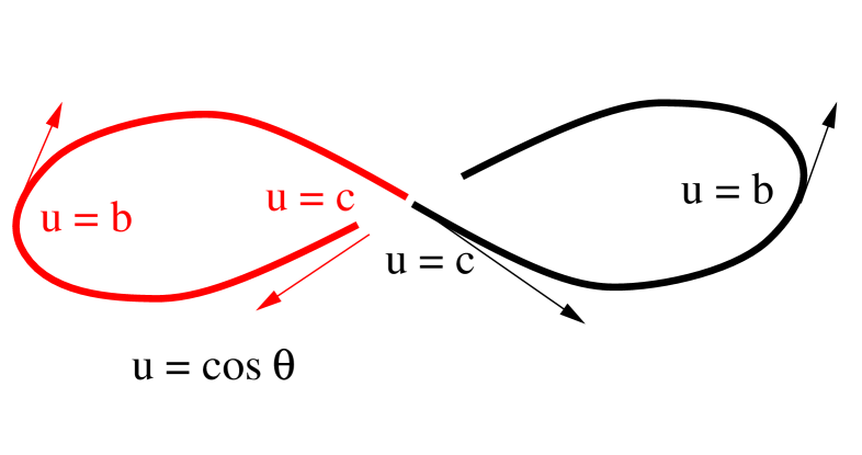
FIG. 1.: The tangent oscillates $c\rightarrow b\rightarrow c\rightarrow b\rightarrow c$. The curve is composed of two symmetric parts.

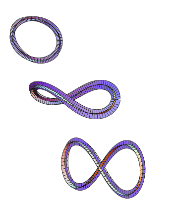
FIG. 2.: The family of curves ranges from the circle in the $XY$ plane to the figure eight in the $YZ$ plane. The perspective is slightly asymmetric to aid visualisation. The “fins” on these, and all other pictured curves, trace out the imbedded $x$ and $y$ axes, and thus depict the twisting of the rod.

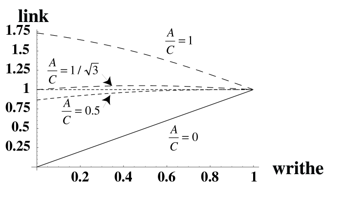
FIG. 3.: The three types of behaviour of ${\cal L}k$ for our writhing family of curves. The ratio $A/C$ controls the plectonemic transition.

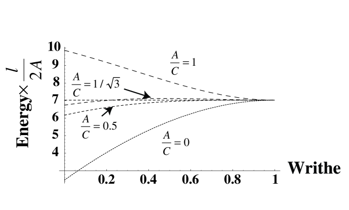
FIG. 4.: The energy as a function of writhe for in the cases plotted in Figure 3. The energy is expressed in units of the combination $2A/l$, where $l$ is the circumference of the writhing loop, and $A$ is the bending modulus. Also shown in this plot is the limiting value of the energy, at the figure eight configuration, which is displayed as a horizontal line.

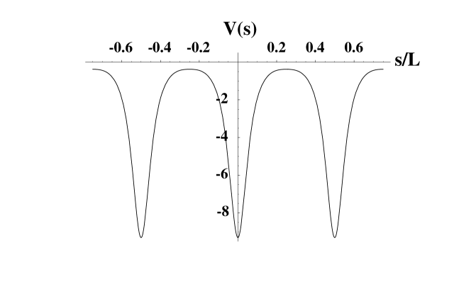
FIG. 5.: Typical potential, as given by Eq. (LABEL:potential1), in the Schrödinger-like equation, (A14), obeyed by fluctuations about the deformed state. The quantity $L$ is the total arclength of the loop.

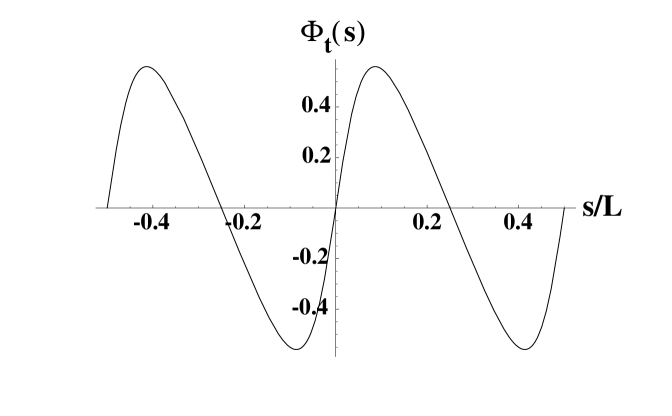
FIG. 6.: The translational mode, $\Phi_{t}(s)$. The normalization of the mode is such that its derivative is unity at $s=0$. The quantity $L$ is the total arclength of the loop.

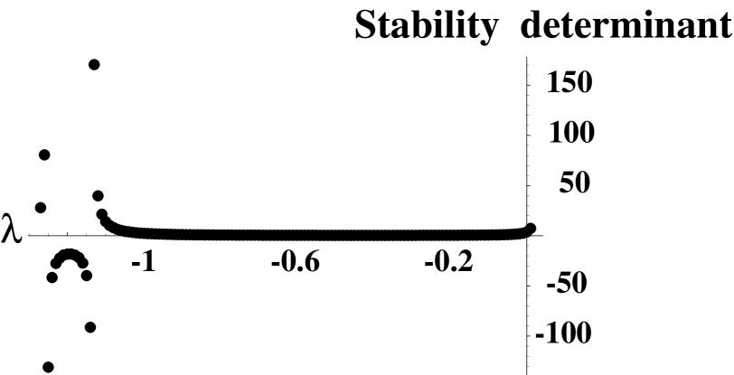
FIG. 7.: The determinant of the four-by-four matrix obtained by sandwiching the response kernel for the deformed loop between four of the five functions associated with the constraints on fluctuations about a solution of the Euler-Lagrange equations for a closed loop. Here the parameter $a$, $b$ and $c$ are equal to 1.14903, 0.145102 and -0.154898, respectively. The poles in the determinant are at the locations of the negative $\lambda$’s associated with unconstrained fluctuations about the extremal solution.

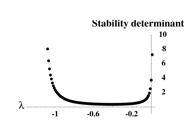
FIG. 8.: A more detailed version of Fig 7, in which the region between the pole at the less negative $\lambda$ and the origin is displayed, to highlight the fact that the determinant does not go through zero when $\lambda$ is negative.

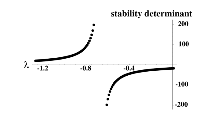
FIG. 9.: The determinant of the one-by-one matrix obtained by sandwiching the response kernel for the deformed loop between the function associated with the constraint of closure in the $y$-direction. The parameters $a$, $b$ and $c$ are equal to 1.14903, 0.145102 and -0.154898, respectively. The pole in the determinant is at the location of the negative $\lambda$ associated with an unconstrained fluctuation about the extremal function.

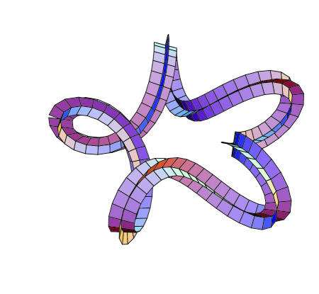
FIG. 10.: The deformation with fivefold symmetry. This represents one of the most “developed” member of the family of fivefold deformed loops. The perspective is off-center to aid the visualization. The actual curve is fivefold symmetric. The “fins” on this curve trace out the imbedded $x$ and $y$ axes, and thus depict the twisting of the rod.

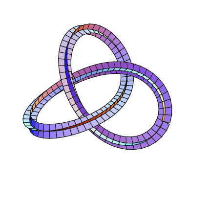
FIG. 11.: A trefoil solution to the Euler-Lagrange equations.This is a member of a family of solutions to the Euler Lagrange equations that knots in this particular way. It represents one of the more strongly “writhed” members of this particular class of solutions.The “fins” on this curve trace out the imbedded $x$ and $y$ axes, and thus depict the twisting of the rod.

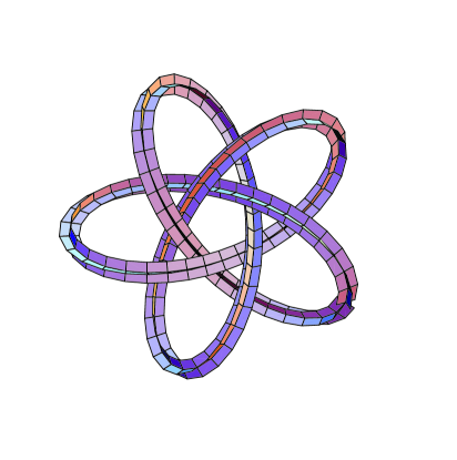
FIG. 12.: A fivefold knotted solution to the Euler-Lagrange equations. This is a member of a family of solutions to the Euler Lagrange equations that knots in this particular way. It represents one of the more strongly “writhed” members of this particular class of solutions. The “fins” on this curve trace out the imbedded $x$ and $y$ axes, and thus depict the twisting of the rod.

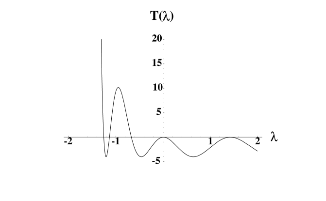
FIG. 13.: The function $T(\lambda)$, as defined by Eq. (E9) for a characteristic supercoiling solution to the Euler-Lagrange equations for a closed loop. Note the zeros of this function at negative values of $\lambda$. The function also passes throught zero at $\lambda=0$ as the result of the existence of the translational mode.

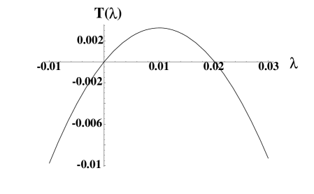
FIG. 14.: A more detailed plot of $T(\lambda)$ in the vicinity of $\lambda=0$. This function passes through zero with a positive slope, and there is, in addition, a zero at small, positive, $\lambda$.

REFERENCES

- [1] Current Address: Department of Structural Biology, Stanford University, Fairchild Building, D-109, Stanford, CA, 94305-5126.
- [2] S. Dustin, et. al. J. Struct. Biol. 107, 15 (1991).
- [3] J. M. Sperrazza, J. C. Register and J. G. Griffith Gene 31, 17 (1984).
- [4] J. Langowski Biophys. Chem. 27, 263 (1987).
- [5] M. Adrian, et. al. EMBO J. 9, 4551 (1990).
- [6] T. C. Boles. J. H. White and N. R. Cozzarelli J. Mol. Biol. 213, 931 (1990).
- [7] J. Bednar, et. al. J. Mol. Biol. 235, 825 (1994).
- [8] T. Odijk and J. Ubbink, Physica A 252, 61 (1998).
- [9] T. R. Strick, J.-F. Allemand, D. Bensimon and V. Croquette Biophys. J. /bf 74, 2016 (1998).
- [10] R. Sinden DNA Structure and Function (Academic Press, San Diego, 1994).
- [11] K. Drlica Trends. Genet. 6, 433 (1990)
- [12] J. C. Wang, Annual Rev. Biochem. 54, 665 (1985)
- [13] M. Gellert, Annual Rev. Biochem. 50, 879 (1981)
- [14] C. J. Benham Biopolymers 22, 2477-2495 (1983).
- [15] M. Le Bret Biopolymers 23, 1835-1867 (1984).
- [16] H. Tsuru and M. Wadati Biopolymers 25 2083-2096 (1986).
- [17] F. Tanaka and H. Takahashi J. Chem. Phys. 83(11) 6017-6026 (1985).
- [18] R. S. Manning , J. H. Maddocks and J. D. Kahn J. Chem. Phys. (submitted) (1996).
- [19] T. Schlick and W. Olsen Science 257, 1110-1115 (1992).
- [20] J. F. Marko and E. D. Siggia Phys. Rev. E 52, 2912-2938 (1995).
- [21] F. Jülicher Phys. Rev. E, 49, 2429 (1994).
- [22] H. Lodish, D. Baltimore, A. Berk, S. L. Zipursky, P. Matsudura, J. Darnell, Molecular Cell Biology (Scientific American Books, New York, 1995).
- [23] B. Fain, J. Rudnick and S. Östlund Phys. Rev. E 55, 7364 (1997).
- [24] F. B. Fuller Proc. Natl. Acad. Sci. USA No.8, 3357-3561 (1978).
- [25] J. H. White Am. J. Math. 91 No.3, 693-727 (1969).
- [26] C. J. Benham Phys. Rev. A 39 2582-2586 (1988)
- [27] W. R. Bauer , R. A. Lund and J. H. White Biochemistry v. 90 833-837, (1992).
- [28] I. Tobias and W. K. Olsen, Biopolymers v. 33 639-646, (1993).
- [29] Z. Nussinov, private communication.
- [30] J. F. Marco and E. D. Siggia Science 265 506-508, (1994).
- [31] S. A. Safran, Stat. Phys. of Surfaces, Interfaces, and Membranes, ch. 6.5, Addison Wesley (1994).
- [32] L. F. Lin, R. E. Depew and J. W. Wang J. Mol. Biol. 106, 439 (1976).
- [33] S. Coleman Aspects of Symmetry (Cambridge University Press, 1985) p. 265-350.