[

Renormalization group analysis of the small-world network model

Abstract

We study the small-world network model, which mimics the transition between regular-lattice and random-lattice behavior in social networks of increasing size. We contend that the model displays a normal continuous phase transition with a divergent correlation length as the degree of randomness tends to zero. We propose a real-space renormalization group transformation for the model and demonstrate that the transformation is exact in the limit of large system size. We use this result to calculate the exact value of the single critical exponent for the system, and to derive the scaling form for the average number of “degrees of separation” between two nodes on the network as a function of the three independent variables. We confirm our results by extensive numerical simulation.

]

Folk wisdom holds that there are “six degrees of separation” between any two human beings on the planet—i.e., a path of no more than six acquaintances linking any person to any other. While the exact number six may not be a very reliable estimate, it does appear that for most social networks quite a short chain is needed to connect even the most distant of the network’s members[1], an observation which has important consequences for issues such as the spread of disease[2], oscillator synchrony[3], and genetic regulatory networks[4]. At first sight this does not seem too surprising a result; random networks have average vertex–vertex distances which increase as the logarithm of the number of vertices and which can therefore be small even in very large networks[5]. However, real social networks are far from random, possessing well-defined locales in which the probability of connection is high and very low probability of connection between two vertices chosen at random. Watts and Strogatz[6] have recently proposed a model of the “small world” which reconciles these observations. Their model does indeed possess well-defined locales, with vertices falling on a regular lattice, but in addition there is a fixed density of random “shortcuts” on the lattice which can link distant vertices. Their principal finding is that only a very small density of such shortcuts is necessary to produce vertex–vertex distances comparable to those found on a random lattice.

In this paper we study the model of Watts and Strogatz using the techniques of statistical physics, and show that it possesses a continuous phase transition in the limit where the density of shortcuts tends to zero. We investigate this transition using a renormalization group (RG) method and calculate the scaling forms and the single critical exponent describing the behavior of the model in the critical region.

Previous studies have concentrated on the one-dimensional version of the small-world model, and we will start with this version too, although we will later generalize our results to higher dimensions. In one dimension the model is defined on a lattice with $L$ sites and periodic boundary conditions (the lattice is a ring). Initially each site is connected to all of its neighbors up to some fixed range $k$ to make a network with average coordination number $z=2k$[7]. Randomness is then introduced by independently rewiring each of the $kL$ connections with probability $p$. “Rewiring” in this context means moving one end of the connection to a new, randomly chosen site. The behavior of the network thus depends on three independent parameters: $L$, $k$ and $p$. In this paper we will study a slight variation on the model in which shortcuts are added between randomly chosen pairs of sites, but no connections are removed from the regular lattice. For sufficiently small $p$ and large $L$ this makes no difference to the mean separation between vertices of the network for $k\geq 2$. For $k=1$ it does make a difference, since the original small-world model is poorly defined in this case—there is a finite probability of a part of the lattice becoming disconnected from the rest and therefore making an infinite contribution to the average distance between vertices, and this makes the distance averaged over all networks for a given value of $p$ also infinite. Our variation does not suffer from this problem and this makes the analysis significantly simpler. In Fig. 1 we show some examples of small-world networks.

We consider the behavior of the model for low density $p$ of shortcuts. The fundamental observable quantity that we measure is the shortest distance between a pair of vertices on the network, averaged both over all pairs on the network and over all possible realizations of the randomness. This quantity, which we denote $\ell$, has two regimes of behavior. For systems small enough that there is much less than one shortcut on the lattice on average, $\ell$ is dominated by the connections of the regular lattice and can be expected to increase linearly with system size $L$. As the lattice becomes larger with $p$ held fixed, the average number of shortcuts will eventually become greater than one and $\ell$ will start to scale as $\log L$. The transition between these two regimes takes place at some intermediate system size $L=\xi$, and from the arguments above we would expect $\xi$ to take a value such that the number of shortcuts $pk\xi\simeq 1$. In other words we expect $\xi$ to diverge in the limit of small $p$ as $\xi\sim p^{-1}$. The quantity $\xi$ plays a role similar to the correlation length in an interacting system in conventional statistical physics, and its divergence leaves the small-world model with no characteristic length scale other than the fundamental lattice spacing. Thus the model possesses a continuous phase transition at $p=0$, and, as we will see, this gives rise to specific finite-size scaling behavior in the region close to the transition. Note that the transition is a one-sided one, since $p$ can never take a value less than zero. In this respect the transition is similar to transitions seen in other one-dimensional systems such as 1D bond or site percolation, or the 1D Ising model.

Barthélémy and Amaral[8] have suggested that the arguments above, although correct in outline, are not correct in detail. They contend that the length-scale $\xi$ diverges as

$$\xi\sim p^{-\tau}$$ (1)

with $\tau$ different from the value of 1 given by the scaling argument. On the basis of numerical results, they conjecture that $\tau=\frac{2}{3}$. Barret[9], on the other hand, has given a simple physical argument which directly contradicts this, indicating that $\tau$ should be greater than or equal to 1. Amongst other things, we demonstrate in this paper that in fact $\tau$ is exactly 1 for all values of $k$.

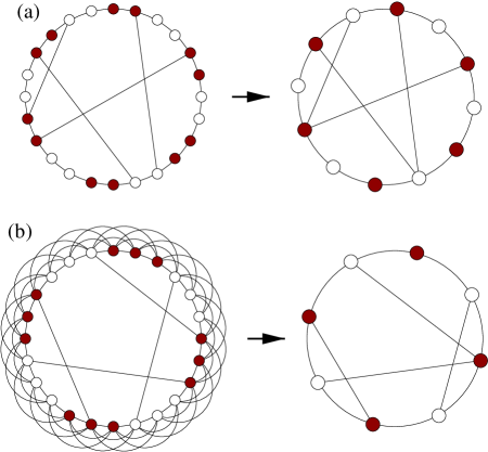
FIG. 1.: The RG transformations used in the calculations described in the text: (a) the transformation used for the $k=1$ system; (b) the transformation used for $k>1$, illustrated in this case for $k=3$. The coloring of the sites indicates how they are grouped under the transformations.

Let us first consider the small-world model for the simplest case $k=1$. As discussed above, the average distance $\ell$ scales linearly with $L$ for $L\ll\xi$ and logarithmically for $L\gg\xi$. If $\xi$ is the only non-trivial length-scale in the problem and is much larger than one (i.e., we are close to the phase transition), this implies that $\ell$ should obey a finite-size scaling law of the form

$$\ell=Lf(L/\xi),$$ (2)

where $f(x)$ is a universal scaling function with the limiting forms

$$f(x)\sim\Bigl{\{}\begin{array}[]{ll}\mbox{constant}&\mbox{for $x\ll 1$}\\ (\log x)/x&\mbox{for $x\gg 1$.}\end{array}$$ (3)

In fact, it is easy to show that the limiting value of $f(x)$ as $x\to 0$ is $\frac{1}{4}$. A scaling law similar to this has been proposed previously by Barthélémy and Amaral[8] for the small-world model, although curiously they suggested that scaling of this type was evidence for the absence of a phase transition in the model, whereas we regard it as the appropriate form for $\ell$ in the presence of one[10].

We now assume that, in the critical region, $\xi$ takes the form (1), and that we do not know the value of the exponent $\tau$. Then we can rewrite Eq. (3) in the form

$$\ell=Lf(p^{\tau}L),$$ (4)

where we have absorbed a multiplicative constant into the argument of $f(x)$, but otherwise it is the same scaling function as before, with the same limits, Eq. (3).

Now consider the real-space RG transformation on the $k=1$ small-world model in which we block sites in adjacent pairs to create a one-dimensional lattice of a half as many sites. (We assume that the lattice size $L$ is even. In fact the transformation works fine if we block in groups of any size which divides $L$.) Two vertices are connected on the renormalized lattice if either of the original vertices in one was connected to either of the original vertices in the other. This includes shortcut connections. The transformation is illustrated in Fig. 1a for a lattice of size $L=24$.

The number of shortcuts on the lattice is conserved under the transformation, so the fundamental parameters $L$ and $p$ renormalize according to

$$L^{\prime}=\mbox{$\frac{1}{2}$}L,\qquad p^{\prime}=2p.$$ (5)

The transformation generates all possible configurations of shortcuts on the renormalized lattice with the correct probability, as we can easily see since the probability of finding a shortcut between any two sites $i$ and $j$ is uniform, independent of $i$ and $j$ both before and after renormalization. The geometry of the shortest path between any two points is unchanged under our transformation. However, the length of the path is, on average, halved along those portions of the path which run around the perimeter of the ring, and remains the same along the shortcuts. For large $L$ and small $p$, the portion of the length along the shortcuts tends to zero and so can be neglected. Thus

$$\ell^{\prime}=\mbox{$\frac{1}{2}$}\ell$$ (6)

in this limit.

Eqs. (5) and (6) constitute the RG equations for this system and are exact for $n\gg 1$ and $p\ll 1$. Substituting into Eq. (4) we then find that

$$\tau={\log(L/L^{\prime})\over\log(p^{\prime}/p)}=1.$$ (7)

Now we turn to the case of $k>1$. To treat this case we define a slightly different RG transformation: we group adjacent sites in groups of $k$, with connections assigned using the same rule as before. The transformation is illustrated in Fig. 1b for a lattice of size $L=24$ with $k=3$. Again the number of shortcuts in the network is preserved under the transformation, which gives the following renormalization equations for the parameters:

$$L^{\prime}=L/k,\qquad p^{\prime}=k^{2}p,\qquad k^{\prime}=1,\qquad\ell^{\prime}=\ell.$$ (8)

Note that, in the limit of large $L$ and small $p$, the mean distance $\ell$ is not affected at all; the number of vertices along the path joining two distant sites is reduced by a factor $k$, but the number of vertices that can be traversed in one step is reduced by the same factor, and the two cancel out. For the same reasons as before, this transformation is exact in the limit of large $L$ and small $p$.

We can use this second transformation to turn any network with $k>1$ into a corresponding network with $k=1$, which we can then treat using the arguments given before. Thus, we conclude, the exponent $\tau=1$ for all values of $k$ and, substituting from Eq. (8) into Eq. (4), the general small-world network must satisfy the scaling form

$$\ell={L\over k}f(pkL).$$ (9)

This form should be correct for $L^{\prime}\gg 1$ and $p^{\prime}\ll 1$, which implies that $L/k\gg 1$ and $k^{2}p\ll 1$. The first of these conditions is trivial—it merely precludes inaccuracies of $\pm k$ in the estimate of $\ell$ because positions on the lattice are rounded off to the nearest multiple of $k$ by the RG transformation. The second condition is interesting however; it is necessary to ensure that the average distance traveled along shortcuts in the network is small compared to the distance traveled around the perimeter of the ring. This condition tells us when we are moving out of the scaling regime close to the transition, which is governed by (9), into the regime of the true random network, for which (9) is badly violated and $\ell$ is known to scale as $\log L/\log k$[5]. It implies that we need to work with values of $p$ which decrease as $k^{-2}$ with increasing $k$ if we wish to see clean scaling behavior, or conversely, that true random-network behavior should be visible in networks with values of $p\simeq k^{-2}$ or greater.

FIG. 2.: Collapse of numerical data for $\ell$ according to Eq. (9) as described in the text. Error bars are in all cases smaller than the data points. Note that the horizontal axis is logarithmic. Inset: the collapse is noticeably poorer for $\tau=\frac{2}{3}$.

We have tested our predictions by extensive numerical simulation of the small-world model. We have calculated exhaustively the minimum distance between all pairs of points on a variety of networks and averaged the results to find $\ell$. We have done this for $k=1$ (coordination number $z=2$) for systems of size $L$ equal to a power of two from $128$ up to $8192$ and $p=1\times 10^{-4}$ up to $3\times 10^{-2}$, and for $k=5$ ($z=10$) with $L=512\ldots 32\,768$ and $p=3\times 10^{-6}\ldots 1\times 10^{-3}$. Each calculation was averaged over 1000 realizations of the randomness. In Fig. 2 we show our results plotted as the values of $\ell k/L$ against $pkL$. Eq. (9) predicts that when plotted in this way, the results should collapse onto a single curve and, as the figure shows, they do indeed do this to a reasonable approximation.

As mentioned above, Barthélémy and Amaral[8] also performed numerical simulations of the small-world model and extracted a value of $\tau=\frac{2}{3}$ for the critical exponent. In the inset of Fig. 2 we show our simulation results for $k=1$ plotted according to Eq. (4) using this value for $\tau$. As the figure shows, the data collapse is significantly poorer in this case than for $\tau=1$. It is interesting to ask then how Barthélémy and Amaral arrived at their result. It seems likely that the problem arises from looking at systems that are too small to show the true scaling behavior. In our calculations, we find good scaling for $L/k\gtrsim 60$. Barthélémy and Amaral examined networks with $k=5$, 10 and 15 ($z=10$, 20, 30) so we should expect to find good scaling behavior for values of $L$ larger than about 600. However, the systems studied by Barthélémy and Amaral ranged in size from about $L=50$ to about $500$ in most cases, and in no case exceeded $L=1000$. Their calculations therefore had either no overlap with the scaling regime, or only a small overlap, and so we would not expect to find behavior typical of the true value of $\tau$ in their results.

It is possible to generalize the calculations presented here to small-world networks built on lattices of dimension $d$ greater than one. For simplicity we consider first the case $k=1$. If we construct a square or (hyper)cubic lattice in $d$ dimensions with linear dimension $L$, connections between nearest neighbor vertices, and shortcuts added with a rewiring probability of $p$, then as before the average vertex–vertex distance scales linearly with $L$ for small $L$, logarithmically for large $L$, and the length-scale $\xi$ of the transition diverges according to Eq. (1) for small $p$. Thus the scaling form (4) applies for general $d$ also. The appropriate generalization of our RG transformation involves grouping sites in square or cubic blocks of side 2, and the quantities $L$, $p$ and $\ell$ then renormalize according to

$$L^{\prime}=\mbox{$\frac{1}{2}$}L,\qquad p^{\prime}=2^{d}p,\qquad\ell^{\prime}=\mbox{$\frac{1}{2}$}\ell.$$ (10)

Thus

$$\tau={\log(L/L^{\prime})\over\log(p^{\prime}/p)}={1\over d}.$$ (11)

As an example, we show in Fig. 3 numerical results for the $d=2$ case, for $L$ equal to a power of two from $64$ up to $512$ (i.e., a little over a quarter of a million vertices for the largest networks simulated) and six different values of $p$ for each system size from $p=3\times 10^{-6}$ up to $1\times 10^{-3}$. The results are plotted according to Eq. (4) with $\tau=\mbox{$\frac{1}{2}$}$ and, as the figure shows, they again collapse nicely onto a single curve.

FIG. 3.: Collapse of numerical data for networks based on the square lattice in two dimensions, as described in the text. Error bars are in all cases smaller than the data points.

A number of generalizations are possible for $k>1$. Perhaps the simplest is to add connections along the principal axes of the lattice between all vertices whose separation is $k$ or less. This produces a graph with average coordination number $z=2dk$. By blocking vertices in square or cubic blocks of edge $k$, we can then transform this system into one with $k=1$. The appropriate generalization of the RG equations (8) is then

$$L^{\prime}=L/k,\quad p^{\prime}=k^{d+1}p,\quad k^{\prime}=1,\quad\ell^{\prime}=\ell,$$ (12)

which gives $\tau=1/d$ for all $k$ and a scaling form of

$$\ell={L\over k}f\bigl{(}(pk)^{1/d}L\bigr{)}.$$ (13)

Alternatively, we could redefine our scaling function $f(x)$ so that $\ell k/L$ is given as a function of $pkL^{d}$. Writing it in this form makes it clear that the number of vertices in the network at the transition from large- to small-world behavior diverges as $(pk)^{-1}$ in any number of dimensions.

Another possible generalization to $k>1$ is to add connections between all sites within square or cubic regions of side $2k$. This gives a different dependence on $k$ in the scaling relation, but $\tau$ still equal to $1/d$.

To conclude, we have studied the small-world network model of Watts and Strogatz using an asymptotically exact real-space renormalization group method. We find that in all dimensions $d$ the model undergoes a continuous phase transition as the density $p$ of shortcuts tends to zero and that the characteristic length $\xi$ diverges according to $\xi\sim p^{-\tau}$ with $\tau=1/d$ for all values of the connection range $k$. We have also deduced the general finite-size scaling law which describes the variation of the mean vertex–vertex separation as a function of $p$, $k$ and the system size $L$. We have performed extensive numerical calculations which confirm our analytic results.

REFERENCES

- [1] S. Milgram, “The small world problem”, Psychol. Today 2, 60–67 (1967).
- [2] L. Sattenspiel and C. P. Simon, “The spread and persistence of infectious diseases in structured populations”, Mathematical Biosciences 90, 367-383 (1988).
- [3] Y. Kuramoto, Chemical Oscillations, Waves and Turbulence, Springer, Berlin (1984).
- [4] S. A. Kauffman, “Metabolic stability and and epigenesis in randomly constructed genetic nets”, J. Theor. Biol. 22, 437–467.
- [5] B. Bollobás, Random Graphs, Academic Press, New York (1985).
- [6] D. J. Watts and S. H. Strogatz, “Collective dynamics of small-world networks”, Nature 393, 440–442 (1998).
- [7] In Ref. [6] is defined to be equal to the coordination number . Here we use to avoid unnecessary factors of 2 in our equations.
- [8] M. Barthélémy and L. A. N. Amaral, “Small-world networks: Evidence for a crossover picture”, cond-mat/9903108.
- [9] A. Barrat, “Comment on ‘Small-world networks: Evidence for a crossover picture’,” cond-mat/9903323.
- [10] Ref. [8] is a little confusing in this respect. It appears the authors may have been referring to the possibility that the system shows a phase transition as the size of the system is varied. This however would not be a sensible suggestion, since it is well-known that systems of finite size do not show sharp phase transitions. The only sensible scenario is a phase transition with varying shortcut probability , which the model does indeed seem to show.