On the theory of Josephson effect in a diffusive tunnel junction

Abstract

Specific features of the equilibrium current-carrying state of a Josephson tunnel junction between diffusive superconductors (with the electron mean free path $l$ smaller than the coherence length $\xi_{0}$) are studied theoretically in the 1D geometry when the current does not spread in the junction banks. It is shown that the concept of weak link with the jump $\Phi\sim 1$ of the order parameter phase exists only for a low transmissivity of the barrier $\Gamma\lesssim\l/\xi_{0}\ll 1$. Otherwise, the presence of the tunnel junction virtually does not affect the distributions of the order parameter modulus and phase. It is found that the Josephson current induces localized states of electron excitations in the vicinity of the tunnel barrier, which are a continuous analog of Andreev levels in a ballistic junction. The depth of the corresponding “potential well” is much greater than the separation between an Andreev level and the continuous energy spectrum boundary for the same transmissivity of the barrier. In contrast to a ballistic junction in which the Josephson current is transported completely by localized excitations, the contribution to current in a diffusive junction comes from whole spectral region near the energy gap boundary, where the density of states differs considerably from its unperturbed value. The correction to the Josephson current $j(\Phi)$ in the second order of the barrier transmissivity, which contains the second harmonic of the phase jump $\Phi$, is calculated and it is found that the true expansion parameter of the perturbation theory for a diffusive junction is not the tunneling probability $\Gamma$, but a much larger parameter $W=(3\xi_{0}/4l)\Gamma$. This simplifies the conditions for the experimental observation of higher harmonics of $j(\Phi)$ in junctions with controllable transmissivity of the barrier.

I Introduction

In recent years, considerable advances have been made in technology of preparing low-resistance tunnel junctions with a comparatively high barrier transmissivity (tunneling probability) $\Gamma$. This primarily applies to controlled break-junctions [1] as well as systems based on 2D electron gas [2], whose conductivity undergoes a crossover from tunnel to metal type upon a change in the barrier parameters. The problem of calculation of the Josephson current through a junction with an arbitrary transmissivity in the ballistic regime (with the electron mean free path $l$ much greater than the coherence length $\xi_{0}$) was solved by many authors [3] on the basis of the model of a single-mode junction with current-carrying banks ensuring a rapid “spreading” of supercurrent and the equality of the order parameter modulus $\Delta$ near the barrier to its bulk value (the “rigidity” condition for $\Delta$).

In the 1D geometry (e.g., a planar junction or a superconducting channel with a tunnel barrier [4]), the problem is complicated considerably due to the change in the order parameter and the quasiparticle energy spectrum in the vicinity of the junction, which makes a contribution to the phase dependence of the current $j(\Phi)$. Antsygina and Svidzinskii [5] determined the corresponding corrections to $j(\Phi)$ of the order of $\Gamma^{2}$ for a pure ($l\gg\xi_{0}$) superconductor in the limit of low transmissivity $\Gamma\ll 1$:

$$\delta j(\Phi)\!=\!-\alpha(T)I(\Delta)\Gamma\left(\sin\Phi\!-\!{1\over 2}\sin 2\Phi\right)\!,\;\;\alpha(T)\!\sim\!1,$$ (1)

$$I(\Delta)=(\pi/4)e\nu_{F}v_{F}\Gamma\Delta=I_{c}(\Delta)/\tanh(\Delta/2T),$$ (2)

where $\nu_{F}$ is the density of states, $v_{F}$ the Fermi velocity, and $I_{c}(\Delta)$ the critical current through the junction.

In a diffusive superconductor (the “dirty” limit $l\ll\xi_{0}=\sqrt{D/2\Delta}$, $D=v_{F}l/3$ is the diffusion constant), the calculation of the Josephson current for an arbitrary $\Gamma$ is hardly possible [6] even in a simple model disregarding the variation of the order parameter in the vicinity of the junction. As a matter of fact, the boundary conditions for isotropic Green’s functions $\hat{g}(\mathchoice{{\hbox{\boldmath$\displaystyle r$}}}{{\hbox{\boldmath$\textstyle r$}}}{{\hbox{\boldmath$\scriptstyle r$}}}{{\hbox{\boldmath$\scriptscriptstyle r$}}},t_{1}t_{2})$ at the junction, obtained by Kupriyanov and Lukichev [9],

$$-l(\hat{g}\nabla\hat{g})_{L}=-l(\hat{g}\nabla\hat{g})_{R}={3\over 4}\left<{\mu d(\mu)\over r(\mu)}\right>\left[\hat{g}_{L},\hat{g}_{R}\right],$$ (3)

where $d(\cos\theta)$ is the tunneling probability for an electron impinging the barrier at an angle $\theta$, and the subscripts $R$ and $L$ mark the value to the right and left of the barrier, are valid only within the first order in small angle-averaged transmissivity $\Gamma=\langle\mu d(\mu)\rangle$. Lambert et al. [10] proved that the derivation of the boundary conditions in the general case ($d\lesssim 1$) is reduced to an analysis of a system of nonlinear integral equations for the terms in the expansion of the averaged Green’s function $\hat{g}(\mathchoice{{\hbox{\boldmath$\displaystyle r$}}}{{\hbox{\boldmath$\textstyle r$}}}{{\hbox{\boldmath$\scriptstyle r$}}}{{\hbox{\boldmath$\scriptscriptstyle r$}}},\mathchoice{{\hbox{\boldmath$\displaystyle p$}}}{{\hbox{\boldmath$\textstyle p$}}}{{\hbox{\boldmath$\scriptstyle p$}}}{{\hbox{\boldmath$\scriptscriptstyle p$}}})=\hat{g}(\mathchoice{{\hbox{\boldmath$\displaystyle r$}}}{{\hbox{\boldmath$\textstyle r$}}}{{\hbox{\boldmath$\scriptstyle r$}}}{{\hbox{\boldmath$\scriptscriptstyle r$}}})+\mathchoice{{\hbox{\boldmath$\displaystyle p\hat{g}$}}}{{\hbox{\boldmath$\textstyle p\hat{g}$}}}{{\hbox{\boldmath$\scriptstyle p\hat{g}$}}}{{\hbox{\boldmath$\scriptscriptstyle p\hat{g}$}}}_{1}(\mathchoice{{\hbox{\boldmath$\displaystyle r$}}}{{\hbox{\boldmath$\textstyle r$}}}{{\hbox{\boldmath$\scriptstyle r$}}}{{\hbox{\boldmath$\scriptscriptstyle r$}}})+\ldots$ over Legendre polynomials. This problem can be solved only for $\Gamma\ll 1$ by expanding the right-hand side of Eq. (3) into a power series in $\Gamma$, which was used in Ref. [10] for calculating the corrections to the Josephson current of the order of $\Gamma^{2}$.

In this paper, we pay attention, first of all, to the fact that the problem of calculation of the current–phase relation for a diffusive junction in the 1D geometry has the sense only in the case of low transmissivity of the barrier. Indeed, simple estimates obtained on the basis of the well-known formula for $j(\Phi)$ in the first order in $\Gamma$,

$$j_{0}(\Phi)=I(\Delta)\tanh(\Delta/2T)\sin\Phi$$ (4)

(which coincides, according to the Anderson theorem, with the Ambegaokar–Baratoff result for a pure superconductor [11]), show that even for small $\Gamma\sim l/\xi_{0}\ll 1$ the critical current through the junction becomes of the order of the bulk thermodynamic critical current $n_{s}ev_{sc}$, where $v_{sc}\sim 1/m\xi_{0}$ is the critical velocity of the condensate, $n_{s}\sim m\nu_{F}D\Delta$ its density, $m$ the electron mass ($\hbar=1$). Thus, for $\Gamma\gg l/\xi_{0}$ the tunnel junction does not play any longer the role of “weak link” with the jump of the order parameter phase $\Phi$ and other features of a Josephson element. This follows even from the boundary conditions Eq. (3) if we use the estimate $\nabla\hat{g}\sim\hat{g}/\xi_{0}$ in the vicinity of the junction, which leads to $[\hat{g}_{L},\hat{g}_{R}]\sim\sin\Phi\sim\xi_{0}/l\Gamma\ll 1$ for $\Gamma\gg l/\xi_{0}$ [12]. This criterion of weak link can be also formulated in terms of the conductance of the system in the normal state: the resistance of the junction must exceed the resistance of a metal layer of thickness $\xi_{0}$.

From this it follows that the parameter

$$W=(3\xi_{0}/4l)\Gamma\gg\Gamma$$ (5)

plays a fundamental role in the theory of Josephson effect for diffusive junction (the factor 3/4 is chosen for convenience of notation). We can attach to this parameter the meaning of the effective tunneling probability for Cooper pairs, which is higher than the conventional probability $\Gamma$ of quasiparticle tunneling. Small values of $W\ll 1$ correspond to “weak link” conditions (Josephson effect); for $W>1$, the presence of a tunnel barrier virtually does not affect the supercurrent flow and the distribution of the order parameter in a diffusive superconductor. Moreover, we can expect that just $W$ and not $\Gamma$ is a true parameter of the expansion of $j(\Phi)$ in the barrier transmissivity. Indeed, the dependence of the Josephson current on the mean free path is absent only within the main approximation in $\Gamma$, Eq. (4) and, therefore, it must be manifested in higher-order terms of the expansion of $j(\Phi)$ in the emergence of additional dimensionless parameter $\xi_{0}/l$ in them, which vanishes at $l\rightarrow\infty$. An analysis of corrections to the current–phase dependence of Eq. (4), carried out in Sec. 4 of this article in the next order in $W$, confirms these considerations and proves that the corrections $\sim\Gamma^{2}$ to the Josephson current obtained in Ref. [10] and associated with the corrections to boundary conditions Eq. (3), are much smaller and insignificant in fact.

Another important result of the analysis of the current-carrying state of a diffusive Josephson junction is the conclusion concerning the emergence of localized states of electron excitations in the vicinity of the barrier. This phenomenon is well known for a ballistic tunnel junction [13, 14] in which discrete energy levels

$$\epsilon_{n}(\Phi)=\pm\Delta(1-d\sin^{2}\Phi/2)^{1/2},$$ (6)

associated with Andreev localization of electron excitations near the jump in the order parameter phase, split from the continuous spectrum in the current-carrying state. A similar phenomenon also takes place in a diffusive junction in which, however, isolated coherent energy levels cannot exist due to electron scattering at impurities and defects. In this case, the most adequate description of the variation of the energy spectrum of excitations is the deformation of their local density of states $N(\epsilon,\mathchoice{{\hbox{\boldmath$\displaystyle r$}}}{{\hbox{\boldmath$\textstyle r$}}}{{\hbox{\boldmath$\scriptstyle r$}}}{{\hbox{\boldmath$\scriptscriptstyle r$}}})=\;\mbox{Re}\;u^{R}(\epsilon,\mathchoice{{\hbox{\boldmath$\displaystyle r$}}}{{\hbox{\boldmath$\textstyle r$}}}{{\hbox{\boldmath$\scriptstyle r$}}}{{\hbox{\boldmath$\scriptscriptstyle r$}}})$ ($u^{R}$ is the diagonal component of the retarded Green’s function for the superconductor) which is assumed for brevity to be normalized to its value $\nu_{F}$ in the normal metal. In the absence of current, the density of states in a homogeneous superconductor has the standard form $N_{0}(\epsilon)=|\epsilon|\Theta(\epsilon^{2}-\Delta^{2})/\sqrt{\epsilon^{2}-\Delta^{2}}$ ($\Theta(x)$ is the Heaviside function) with root singularities at the gap boundaries. In the current state, the momentum $p_{s}$ of the superfluid condensate plays the role of a depairing factor smoothing the singularities of $N(\epsilon)$ and reducing the energy gap $2\epsilon_{\ast}$ by $\Delta-\epsilon_{\ast}(p_{s})\sim(Dp_{s}^{2})^{2/3}$ [15]. In the vicinity of a weak link, a similar (and main) factor of the energy gap suppression is the phase jump $\Phi$ which leads to the formation of a “potential well” around the junction having a width of the order of $\xi_{0}$ and containing localized excitations with an energy $|\epsilon|<\Delta$ (see Sec. 3). In contrast to the ballistic case, the Josephson transport in a diffusive junction is performed not only by the states in the potential well, but by excitations within the whole energy region near the gap edge where the density of states differs significantly from the unperturbed value.

II Equations for Green’s function of a low-transparent Josephson junction

In order to calculate the density of states and equilibrium supercurrent

$$j={e\over 4}\nu_{F}v_{F}D\int^{+\infty}_{-\infty}\!\!\!\!d\epsilon f_{0}(\epsilon)\mbox{Tr}\sigma_{z}(\hat{g}^{R}\nabla\hat{g}^{R}\!-\!\hat{g}^{A}\nabla\hat{g}^{A})(\epsilon)$$ (7)

we must solve equations for the matrix retarded (advanced) Green’s functions $\hat{g}^{R,A}(\mathchoice{{\hbox{\boldmath$\displaystyle r$}}}{{\hbox{\boldmath$\textstyle r$}}}{{\hbox{\boldmath$\scriptstyle r$}}}{{\hbox{\boldmath$\scriptscriptstyle r$}}},\epsilon)$ averaged over the ensemble of scatterers:

$$[\sigma_{z}\epsilon+\Delta\exp(i\sigma_{z}\chi)i\sigma_{y},\hat{g}]=iD\nabla(\hat{g}\nabla\hat{g}),$$ (8)

Here $\Delta$ and $\chi$ are the modulus and phase of the order parameter and $f_{0}(\epsilon)=(1/2)(1+\tanh(\epsilon/2T))$ is the equilibrium distribution function.

According to the normalization condition $\hat{g}^{2}=1$ for the Green’s function, the matrix $\hat{g}$ can be presented as $\hat{g}=\mathchoice{{\hbox{\boldmath$\displaystyle\sigma u$}}}{{\hbox{\boldmath$\textstyle\sigma u$}}}{{\hbox{\boldmath$\scriptstyle\sigma u$}}}{{\hbox{\boldmath$\scriptscriptstyle\sigma u$}}}$, where $\textstyle\sigma$ is the vector formed by Pauli matrices. Using the well-known relations $(\mathchoice{{\hbox{\boldmath$\displaystyle\sigma a$}}}{{\hbox{\boldmath$\textstyle\sigma a$}}}{{\hbox{\boldmath$\scriptstyle\sigma a$}}}{{\hbox{\boldmath$\scriptscriptstyle\sigma a$}}})(\mathchoice{{\hbox{\boldmath$\displaystyle\sigma b$}}}{{\hbox{\boldmath$\textstyle\sigma b$}}}{{\hbox{\boldmath$\scriptstyle\sigma b$}}}{{\hbox{\boldmath$\scriptscriptstyle\sigma b$}}})=\mathchoice{{\hbox{\boldmath$\displaystyle ab$}}}{{\hbox{\boldmath$\textstyle ab$}}}{{\hbox{\boldmath$\scriptstyle ab$}}}{{\hbox{\boldmath$\scriptscriptstyle ab$}}}+i\mathchoice{{\hbox{\boldmath$\displaystyle\sigma$}}}{{\hbox{\boldmath$\textstyle\sigma$}}}{{\hbox{\boldmath$\scriptstyle\sigma$}}}{{\hbox{\boldmath$\scriptscriptstyle\sigma$}}}[\mathchoice{{\hbox{\boldmath$\displaystyle a$}}}{{\hbox{\boldmath$\textstyle a$}}}{{\hbox{\boldmath$\scriptstyle a$}}}{{\hbox{\boldmath$\scriptscriptstyle a$}}}\times\mathchoice{{\hbox{\boldmath$\displaystyle b$}}}{{\hbox{\boldmath$\textstyle b$}}}{{\hbox{\boldmath$\scriptstyle b$}}}{{\hbox{\boldmath$\scriptscriptstyle b$}}}]$, $[\sigma_{z},\mathchoice{{\hbox{\boldmath$\displaystyle\sigma$}}}{{\hbox{\boldmath$\textstyle\sigma$}}}{{\hbox{\boldmath$\scriptstyle\sigma$}}}{{\hbox{\boldmath$\scriptscriptstyle\sigma$}}}]=2i[\mathchoice{{\hbox{\boldmath$\displaystyle\sigma$}}}{{\hbox{\boldmath$\textstyle\sigma$}}}{{\hbox{\boldmath$\scriptstyle\sigma$}}}{{\hbox{\boldmath$\scriptscriptstyle\sigma$}}}\times\mathchoice{{\hbox{\boldmath$\displaystyle s$}}}{{\hbox{\boldmath$\textstyle s$}}}{{\hbox{\boldmath$\scriptstyle s$}}}{{\hbox{\boldmath$\scriptscriptstyle s$}}}]$, where $\textstyle s$ is the unit vector of “isotopic spin” directed along the $z$-axis in the space of Pauli matrices, we can obtain from Eqs. (3) and (8) the following equations and the boundary conditions for the vector Green’s function $\textstyle u$:

$$\epsilon[\mathchoice{{\hbox{\boldmath$\displaystyle s$}}}{{\hbox{\boldmath$\textstyle s$}}}{{\hbox{\boldmath$\scriptstyle s$}}}{{\hbox{\boldmath$\scriptscriptstyle s$}}}\times\mathchoice{{\hbox{\boldmath$\displaystyle u$}}}{{\hbox{\boldmath$\textstyle u$}}}{{\hbox{\boldmath$\scriptstyle u$}}}{{\hbox{\boldmath$\scriptscriptstyle u$}}}]+i\Delta[\mathchoice{{\hbox{\boldmath$\displaystyle\chi$}}}{{\hbox{\boldmath$\textstyle\chi$}}}{{\hbox{\boldmath$\scriptstyle\chi$}}}{{\hbox{\boldmath$\scriptscriptstyle\chi$}}}\times\mathchoice{{\hbox{\boldmath$\displaystyle u$}}}{{\hbox{\boldmath$\textstyle u$}}}{{\hbox{\boldmath$\scriptstyle u$}}}{{\hbox{\boldmath$\scriptscriptstyle u$}}}]=(D/2)\nabla[\mathchoice{{\hbox{\boldmath$\displaystyle u$}}}{{\hbox{\boldmath$\textstyle u$}}}{{\hbox{\boldmath$\scriptstyle u$}}}{{\hbox{\boldmath$\scriptscriptstyle u$}}}\times\nabla\mathchoice{{\hbox{\boldmath$\displaystyle u$}}}{{\hbox{\boldmath$\textstyle u$}}}{{\hbox{\boldmath$\scriptstyle u$}}}{{\hbox{\boldmath$\scriptscriptstyle u$}}}],\;\;\mathchoice{{\hbox{\boldmath$\displaystyle u$}}}{{\hbox{\boldmath$\textstyle u$}}}{{\hbox{\boldmath$\scriptstyle u$}}}{{\hbox{\boldmath$\scriptscriptstyle u$}}}^{2}=1,$$ (9)

$$\xi_{0}[\mathchoice{{\hbox{\boldmath$\displaystyle u$}}}{{\hbox{\boldmath$\textstyle u$}}}{{\hbox{\boldmath$\scriptstyle u$}}}{{\hbox{\boldmath$\scriptscriptstyle u$}}}\times\nabla\mathchoice{{\hbox{\boldmath$\displaystyle u$}}}{{\hbox{\boldmath$\textstyle u$}}}{{\hbox{\boldmath$\scriptstyle u$}}}{{\hbox{\boldmath$\scriptscriptstyle u$}}}]_{L,R}=2W[\mathchoice{{\hbox{\boldmath$\displaystyle u$}}}{{\hbox{\boldmath$\textstyle u$}}}{{\hbox{\boldmath$\scriptstyle u$}}}{{\hbox{\boldmath$\scriptscriptstyle u$}}}_{L}\times\mathchoice{{\hbox{\boldmath$\displaystyle u$}}}{{\hbox{\boldmath$\textstyle u$}}}{{\hbox{\boldmath$\scriptstyle u$}}}{{\hbox{\boldmath$\scriptscriptstyle u$}}}_{R}],$$ (10)

where $\mathchoice{{\hbox{\boldmath$\displaystyle\chi$}}}{{\hbox{\boldmath$\textstyle\chi$}}}{{\hbox{\boldmath$\scriptstyle\chi$}}}{{\hbox{\boldmath$\scriptscriptstyle\chi$}}}=(\sin\chi,\cos\chi,0)$ is the symbolic vector of the order parameter phase.

Singling out the component of the vector $\textstyle u$ along the direction $\textstyle s$: $\mathchoice{{\hbox{\boldmath$\displaystyle u$}}}{{\hbox{\boldmath$\textstyle u$}}}{{\hbox{\boldmath$\scriptstyle u$}}}{{\hbox{\boldmath$\scriptscriptstyle u$}}}=\mathchoice{{\hbox{\boldmath$\displaystyle s$}}}{{\hbox{\boldmath$\textstyle s$}}}{{\hbox{\boldmath$\scriptstyle s$}}}{{\hbox{\boldmath$\scriptscriptstyle s$}}}u+i\mathchoice{{\hbox{\boldmath$\displaystyle v$}}}{{\hbox{\boldmath$\textstyle v$}}}{{\hbox{\boldmath$\scriptstyle v$}}}{{\hbox{\boldmath$\scriptscriptstyle v$}}}$ ($\mathchoice{{\hbox{\boldmath$\displaystyle vs$}}}{{\hbox{\boldmath$\textstyle vs$}}}{{\hbox{\boldmath$\scriptstyle vs$}}}{{\hbox{\boldmath$\scriptscriptstyle vs$}}}=0$), we project Eq. (9) onto the $(x,y)$-plane in the space of Pauli matrices:

$$\epsilon\mathchoice{{\hbox{\boldmath$\displaystyle v$}}}{{\hbox{\boldmath$\textstyle v$}}}{{\hbox{\boldmath$\scriptstyle v$}}}{{\hbox{\boldmath$\scriptscriptstyle v$}}}-\Delta u\mathchoice{{\hbox{\boldmath$\displaystyle\chi$}}}{{\hbox{\boldmath$\textstyle\chi$}}}{{\hbox{\boldmath$\scriptstyle\chi$}}}{{\hbox{\boldmath$\scriptscriptstyle\chi$}}}=(iD/2)\nabla(u\nabla\mathchoice{{\hbox{\boldmath$\displaystyle v$}}}{{\hbox{\boldmath$\textstyle v$}}}{{\hbox{\boldmath$\scriptstyle v$}}}{{\hbox{\boldmath$\scriptscriptstyle v$}}}-\mathchoice{{\hbox{\boldmath$\displaystyle v$}}}{{\hbox{\boldmath$\textstyle v$}}}{{\hbox{\boldmath$\scriptstyle v$}}}{{\hbox{\boldmath$\scriptscriptstyle v$}}}\nabla u),\;\;u^{2}-\mathchoice{{\hbox{\boldmath$\displaystyle v$}}}{{\hbox{\boldmath$\textstyle v$}}}{{\hbox{\boldmath$\scriptstyle v$}}}{{\hbox{\boldmath$\scriptscriptstyle v$}}}^{2}=1$$ (11)

and introduce the unit vector $\mathchoice{{\hbox{\boldmath$\displaystyle\psi$}}}{{\hbox{\boldmath$\textstyle\psi$}}}{{\hbox{\boldmath$\scriptstyle\psi$}}}{{\hbox{\boldmath$\scriptscriptstyle\psi$}}}=(\sin\psi,\cos\psi,0)$ directed along $\textstyle v$: $\mathchoice{{\hbox{\boldmath$\displaystyle v$}}}{{\hbox{\boldmath$\textstyle v$}}}{{\hbox{\boldmath$\scriptstyle v$}}}{{\hbox{\boldmath$\scriptscriptstyle v$}}}=\mathchoice{{\hbox{\boldmath$\displaystyle\psi$}}}{{\hbox{\boldmath$\textstyle\psi$}}}{{\hbox{\boldmath$\scriptstyle\psi$}}}{{\hbox{\boldmath$\scriptscriptstyle\psi$}}}v$, where $\psi(\mathchoice{{\hbox{\boldmath$\displaystyle r$}}}{{\hbox{\boldmath$\textstyle r$}}}{{\hbox{\boldmath$\scriptstyle r$}}}{{\hbox{\boldmath$\scriptscriptstyle r$}}},\epsilon)$ is the phase of “anomalous” Green’s function $v$ ($\nabla\mathchoice{{\hbox{\boldmath$\displaystyle\psi$}}}{{\hbox{\boldmath$\textstyle\psi$}}}{{\hbox{\boldmath$\scriptstyle\psi$}}}{{\hbox{\boldmath$\scriptscriptstyle\psi$}}}=[\mathchoice{{\hbox{\boldmath$\displaystyle\psi$}}}{{\hbox{\boldmath$\textstyle\psi$}}}{{\hbox{\boldmath$\scriptstyle\psi$}}}{{\hbox{\boldmath$\scriptscriptstyle\psi$}}}\times\mathchoice{{\hbox{\boldmath$\displaystyle s$}}}{{\hbox{\boldmath$\textstyle s$}}}{{\hbox{\boldmath$\scriptstyle s$}}}{{\hbox{\boldmath$\scriptscriptstyle s$}}}]\nabla\psi$). The obtained system of scalar equations is a possible representation of Usadell equations:

$$\epsilon v\!-\!\Delta u\cos(\psi\!-\!\chi)\!=\!{i\over 2}D\left[\nabla(u\nabla\!v\!-\!v\nabla\!u)\!-\!uv(\nabla\!\psi)^{2}\right]\!,$$ (12)

$$\Delta v\sin(\psi-\chi)=(iD/2)\nabla(v^{2}\nabla\psi),$$ (13)

$$u^{2}-v^{2}=1,$$ (14)

and its solutions determine the supercurrent

$$j(\Phi)=-e\nu_{F}D\int_{-\infty}^{+\infty}d\epsilon f_{0}\;\mbox{Im}\;(v^{R})^{2}\nabla\psi^{R}.$$ (15)

Choosing the coordinate axis $x$ orthogonally to the contact plane $x=0$ ($\chi(+0)=-\chi(-0)=\Phi/2$) and taking into account the continuity of Green’s function and antisymmetry of their derivatives, we can easily obtain from Eq. (10) the boundary conditions to Eqs. (12), (13) for $x\rightarrow+0$:

$$\xi_{0}(u\nabla v-v\nabla u)(0)=4Wu(0)v(0)\sin^{2}\psi(0),$$ (16)

$$\xi_{0}\nabla\psi(0)=2W\sin 2\psi(0).$$ (17)

Far away from the junction, the behavior of the order parameter and Green’s function phases is described by linear asymptotic form corresponding to the given value of current

$$\chi(+\infty)\!=\!\psi(+\infty)\!=\!\chi_{\infty}+2p_{s}x,\;\;p_{s}\!=\!(W/\xi_{0})\sin\Phi,$$ (18)

i.e., of the superfluid momentum $p_{s}$ whose magnitude is determined in the main approximation by the condition of equality of the current Eq. (4) through the junction to its value $j=\pi e\nu_{F}Dp_{s}\Delta\tanh(\Delta/2T)$ in the bulk of the metal. The Green’s functions tend to their asymptotic values satisfying Eqs. (12)–(14) for $\psi=\chi$ and $\nabla u=\nabla v=0$.

Using the parametrization $u=\cosh\theta,v=\sinh\theta$, which takes into account the normalization condition Eq. (14), we can put in correspondence to the vector Green’s function $\textstyle u$ the following geometrical image [16]. The unit vector $\textstyle u$ in a normal metal is directed along the isospin axis $z$ (which corresponds to a purely electron or hole state of excitation of a Fermi gas), while in a superconductor this vector is deflected from the axis through an imaginary angle $i\theta$ and turned around it through the azimuthal angle $\psi$. In the spatially homogeneous case, this angle obviously coincides with the phase of the order parameter ($\psi=\chi$), and the scalar Green’s functions $u$ and $v$ are described by the formulas

$$u^{R,A}\!=\!\cosh\theta_{s}\!=\!{\epsilon\over\sqrt{(\epsilon\pm i0)^{2}-\Delta^{2}}},\;\;v^{R,A}\!=\!\sinh\theta_{s},$$ (19)

where $\pm i0$ defines the position of singularities of the retarded (advanced) Green’s function in the complex plane $\epsilon$, and the square root in Eq. (20) is defined so that $u^{R,A}\rightarrow\pm 1$ for $\epsilon\rightarrow+\infty$.

Eqs. (12)–(14) for Green’s functions should be supplemented by the self-consistency conditions for the modulus and phase of the order parameter:

$$\Delta=\lambda\int^{+\infty}_{-\infty}d\epsilon f_{0}\;\mbox{Re}\;v^{R},$$ (20)

$$\int_{-\infty}^{+\infty}d\epsilon f_{0}\;\mbox{Re}\;v^{R}\sin(\psi^{R}-\chi)=0,$$ (21)

where $\lambda$ is the constant of superconducting interaction. Taking into account the current conservation law, Eqs. (13) and (21), it is convenient to calculate the value of current at the barrier ($x\rightarrow+0$) by expressing $\nabla\psi(0)$ in Eq. (15) with the help of Eq. (17) through the phase jump $2\psi(0)$:

$$j(\Phi)\!=\!-{e\over 2}\nu_{F}v_{F}\Gamma\!\int_{-\infty}^{+\infty}\!\!\!d\epsilon f_{0}\;\mbox{Im}\;(v^{R}(0))^{2}\sin 2\psi^{R}(0),$$ (22)

which allows us to single out explicitly the small parameter of the theory, i.e., the barrier transmissivity $\Gamma$. It can easily be verified that in the main approximation using the unperturbed values of Green’s function of Eq. (19) and phase $\psi(0)\approx\chi(0)=\Phi/2$, Eq. (22) leads to the result of Eq. (4).

A simplifying factor in the case of a low transmissivity of the barrier is that the quantities $\psi-\chi$ and $\nabla\psi$ proportional to the current through the junction are small (see Eqs. (17) and (13)), and hence we can omit in Eq. (12) the terms quadratic in $W$ and containing the phase gradients. Replacing $\psi(0)\approx\chi(0)=\Phi/2$ in the boundary conditions Eqs. (16), (17), to the same degree of accuracy, we obtain the equation and the boundary conditions for the parameter $\theta$:

$$\epsilon\sinh\theta-\Delta(x)\cosh\theta=(iD/2)\nabla^{2}\theta,$$ (23)

$$\xi_{0}\nabla\theta(0)=2W\sinh 2\theta(0)\sin^{2}\Phi/2,\;\;\theta(+\infty)=\theta_{s}.$$ (24)

Direct application of the perturbation theory to the solution of Eq. (23) ($\theta(x)=\theta_{0}+\theta_{1}(x)$, $\Delta(x)=\Delta_{0}+\Delta_{1}(x)$) leads to an expression for the correction $\theta_{1}(x)$ containing nonintegrable singularities at the gap boundaries, and as a consequence, to the divergence of the corresponding correction to the Josephson current Eq. (4). This is associated with the emergence of localized states of quasiparticles at a tunnel junction in the current-carrying state mentioned in Introduction and considered in the next section.

III Localized states at a tunnel barrier

It will be proved below that the depth of the “potential well” in the vicinity of the barrier is much larger than the scale of variation of the order parameter. Consequently, it is sufficient to confine an analysis of the behavior of the density of states to the model with a constant $\Delta$, in which Eq. (23) has a simple solution describing the attenuation of perturbations of Green’s functions at a distance $\sim\xi_{0}$ from the barrier:

$$\tanh{\theta(x)-\theta_{s}\over 4}=\tanh{\theta(0)-\theta_{s}\over 4}\exp(-k_{\epsilon}|x|),$$ (26)

$$k^{-2}_{\epsilon}=i\xi_{0}^{2}\sinh\theta_{s},\;\;\mbox{Re}\;k_{\epsilon}>0.$$ (27)

The quantity $\theta(0)$ satisfies the boundary condition following from Eqs. (24) and (25):

$$k_{\epsilon}\xi_{0}\sinh{\theta_{s}\!-\!\theta(0)\over 2}\!=\!\gamma\sinh 2\theta(0),\;\gamma\!=\!W\sin^{2}{\Phi\over 2}\!\ll\!1,$$ (28)

which can be reduced to the eighth-power algebraic equation in $z=\exp\theta(0)$:

$$2z^{3}(z-z_{s})^{2}=i\gamma^{2}(z_{s}^{2}-1)(z^{4}-1)^{2},\;\;z_{s}=\exp\theta_{s}.$$ (29)

In the general case (for an arbitrary $\epsilon$), the solution of Eq. (27) can be obtained only numerically, but the presence of the small parameter $\gamma$ in (26) and (27) makes it possible to apply the perturbation theory. Far away from the spectrum boundary, we can put $\theta(0)=\theta_{s}$ on right-hand side of (26), which leads to the following expression for the correction to the density of states at the barrier:

$$N(\epsilon,0)-N_{0}(\epsilon)=-2\gamma\;\mbox{Re}\left(\sqrt{i\sinh^{3}\theta_{s}}\sinh 2\theta_{s}\right),$$ (30)

that becomes obviously inapplicable for $|\epsilon|\rightarrow\Delta$, where $|\theta_{s}|\rightarrow\infty$. In this region, we must apply the improved perturbation theory (IPT) by putting $|z|,|z_{s}|\gg 1$ for an arbitrary (not necessarily small) value of $z-z_{s}$. This not only reduces the power of the general Eq. (27), but also allows us to write it in a universal form which does not contain the depairing parameter $\gamma$:

$$(y\sqrt{E}-1)^{2}=iy^{5},$$ (32)

$$y\!=\!z/\beta\sqrt{2},\;E\!=\!\beta^{2}(\epsilon\!-\!\Delta)/\Delta,\;\beta\!=\!(2/\gamma)^{1/5}\gg 1,$$ (33)

Relations Eq. (29) show that the increase in the density of states is bounded by a quantity of the order of $\beta\sim W^{-2/5}$ as we approach the spectrum boundary. Thus, the range of applicability of the conventional perturbation theory, Eq. (28), is determined by the condition $(\epsilon-\Delta)/\Delta\gg\beta^{-2}$ and overlaps with the region of applicability $(\epsilon-\Delta)/\Delta\ll 1$ of the IPT. The boundary $\epsilon_{\ast}$ of the spectrum (the position of the bottom of the potential well), below which the density of states vanishes, corresponds to the emergence of a purely imaginary root of Eq. (29a) at the point $E_{\ast}=-(25/6)(2/3)^{1/5}\approx-3.842$:

$$\epsilon_{\ast}(\Phi)\!=\!\Delta\!\!\left[\!1\!-\!C\!\!\left(\!\!W\sin^{2}\!{\Phi\over 2}\!\right)^{\!4/5}\right]\!\!,\;C\!=\!{25\over 3\!\cdot\!6^{1/5}}\!\approx\!5.824.$$ (34)

The dependence of the position of the spectrum boundary on the phase jump at the junction is illustrated by Fig. 1 in which a similar dependence of the position of the Andreev level Eq. (6) in a junction between pure superconductors is shown for comparison. It should be noted that the scale of variation of $\epsilon_{\ast}(\Phi)$ is much larger than the splitting of the Andreev level from the boundary of the continuous spectrum for the same barrier transmissivity. This is associated with the large value of the depairing parameter $\gamma$ in the diffusive junction as compared to the splitting parameter $\Gamma$ of the Andreev level as well as with the large numerical value of the constant $C$ defining the shift of the spectrum boundary Eq. (30). Fig. 2 shows the results of numerical calculation of the density of states at the junction on the basis of the general formula Eq. (27) for different values of the depairing parameter, which show that in addition of the root singularity ($\sim\sqrt{\epsilon-\epsilon_{\ast}}$) at the spectrum boundary, the quantity $N(\epsilon)$ has a “beak-type” root singularity for $\epsilon=\Delta$. Its physical nature is associated with an infinite increase in the attenuation length $k_{\epsilon}^{-1}$ of the perturbation of Green’s function in the bulk of the metal, Eq. (25), within the vicinity of the gap boundary.

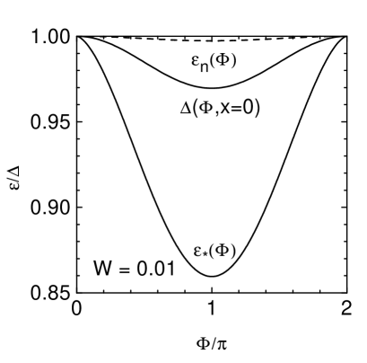
FIG. 1.: Phase dependence of the position of the bottom of the “potential well” $\epsilon_{\ast}$, Eq. (30), and the order parameter $\Delta(0)$, Eq. (48), in the vicinity of the tunnel junction (solid curves) at $T=0,W=0.01$ and $\xi_{0}/l=5$. The dashed curve shows for comparison the position of the Andreev level in a pure single-mode junction, Eq. (5), for the same barrier transmissivity.

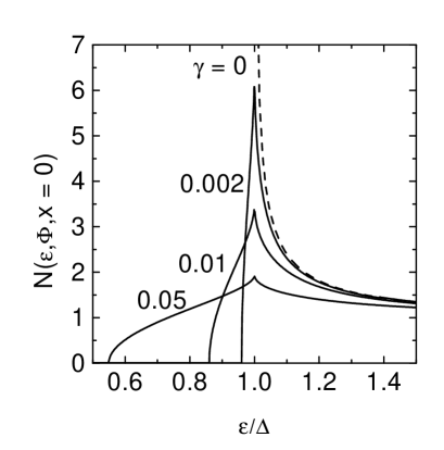
FIG. 2.: Dependence of the density of states $N(\epsilon,\Phi,0)$ at the tunnel junction on the energy of quasiparticles for various values of the depairing parameter $\gamma=W\sin^{2}(\Phi/2)$ (solid curves). The dashed curve shows the energy dependence of the unperturbed density of states $N_{0}(\epsilon)$.

For $\epsilon_{\ast}<\epsilon<\Delta$, the density of states decreases exponentially with increasing distance from the junction (Fig. 3), which corresponds qualitatively to the image of the potential well of depth $\Delta-\epsilon_{\ast}$ and of width $\sim\xi_{0}$ with excitations localized in it.

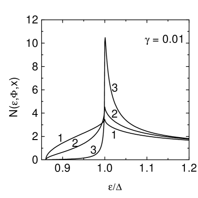
FIG. 3.: Energy dependence of the density of states $N(\epsilon,\Phi,0)$ for $\gamma=0.01$ at different distances $x$ from a diffusive tunnel junction: 0 (curve 1), $\xi_{0}$ (curve 2), and $5\xi_{0}$ (curve 3).

It is well known that the Josephson current is carried through a ballistic junction by localized excitations only and can be presented in the following form:

$$j(\Phi)=-2e\sum_{n}{\partial\epsilon_{n}(\Phi)\over\partial\Phi}\tanh{\epsilon_{n}(\Phi)\over 2T},$$ (35)

where the index $n$ labels Andreev levels. At the same time, Eq. (22) for current expressed in the IPT approximation in terms of the reduced variables of Eq. (29),

$$j(\Phi)\!\approx\!-I(\Delta)\tanh{\Delta\over 2T}\sin\Phi\!\!\!\!\int\limits_{E_{\ast}(\Phi)}^{\infty}\!\!\!\!{dE\over\pi}\mbox{Im}\left(y^{R}\right)^{2}\!\!=\!j_{0}(\Phi),$$ (36)

shows that the charge transfer in a diffusive junction is performed not only by the states within the potential well ($E<0,\epsilon<\Delta$), but also by the excitations with energy $\epsilon>\Delta$ in the region $\epsilon-\Delta\sim\Delta\beta^{-2}$, where the density of states differs significantly from the unperturbed value $N_{0}(\epsilon)$. It should be noted in this connection that Argaman [17] proposed an analog of Eq. (31) for a diffusive system, which can be obtained by the replacement of the energy $\epsilon_{n}(\Phi)$ of Andreev levels by the local value $\epsilon(\xi,\Phi,x)$ of the excitation energy for $x=0$, which is adiabatically deformed by supercurrent, using instead of the discrete number $n$ the continuous variable

$$\xi=\int_{\textstyle{\epsilon_{\ast}(\Phi)}}^{\textstyle{\epsilon(\xi,\Phi,x)}}d\epsilon^{\prime}N(\epsilon^{\prime},\Phi,x)$$ (37)

viz., the number of states with an energy smaller than $\epsilon$ ($\xi=\Theta(\epsilon^{2}-\Delta^{2})\sqrt{\epsilon^{2}-\Delta^{2}}$ for a homogeneous superconductor) [18]. One can assume that the contributions from the bound and delocalized states to the Josephson current are taken into account simultaneously by the formula

$$j(\Phi)=-2e\nu_{F}\int_{0}^{\infty}d\xi\;{\partial\epsilon(\xi,\Phi,0)\over\partial\Phi}\tanh{\epsilon(\xi,\Phi,0)\over 2T},$$ (38)

which, however, leads to correct results only in the case of a homogeneous current-carrying state (where $\nabla\chi$ plays the role of $\Phi$) or a wide $SNS$-junction (with a width $L\gg\xi_{0}$ of the normal layer) and is inapplicable for a narrow bridge and tunnel junction. Nevertheless, the consideration of the function $\epsilon(\xi,\Phi,x)$ is useful in these cases also since this allows us to visualize the variation of the energy distribution of quasiparticle states in the vicinity of the junction (Fig. 4).

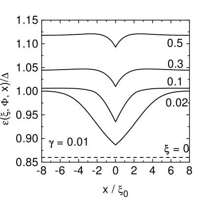
FIG. 4.: Lines corresponding to the number of states of quasiparticles $\xi(\epsilon,\Phi,x)={\rm const}$ (Eq. (33)) for $\gamma=0.01$ in the vicinity of the junction. The dashed line shows the position of the bottom of the “potential well” ($\xi=0,\epsilon=\epsilon_{\ast}(\Phi)$).

IV Current–phase dependence for a junction in the second order in $W$

Although the modified perturbation theory for Green’s function in the energy representation described in the preceding section is the most physically obvious method operating with actual excitation energies, it leads to considerable formal difficulties in the calculation of corrections to the Josephson current Eq. (4). Indeed, it was shown in the previous section that the expression for $j(\Phi)$ calculated on the basis of the IPT for Green’s functions, Eq. (32), coincides with Eq. (4) since the small IPT parameter $\beta^{-2}$ cancels out as we go over to the reduced variables of Eq. (29). Thus, in order to calculate the corrections to Eq. (4) we are interested in, we must leave the approximation of Eq. (29) that describes the behavior of Green’s functions correctly only in a narrow vicinity of singularity in the density of states. For this purpose, it is convenient to use the formalism of temperature Green’s functions by going over from integration over energy in Eqs. (20)–(22) to summation over the Matsubara frequencies $\omega_{n}=\pi T(2n+1),n=0,\pm 1,\pm 2,\ldots$:

$$j(\Phi)=-\pi e\nu_{F}v_{F}\Gamma T\sum_{\omega_{n}>0}\;\mbox{Re}\;v^{2}(0)\sin 2\psi(0),$$ (39)

$$\Delta(x)=-2\pi\lambda T\sum_{\omega_{n}>0}\;\mbox{Im}\;v(x)$$ (40)

and making the substitution $\epsilon\rightarrow i\omega_{n}$ in Eq. (23). This allows us to avoid divergences of the type of Eq. (28) in the perturbation theory which, unlike the IPT, makes it possible to take into account the coordinate dependence $\Delta(x)$.

It is expedient to use as the main approximation in the asymptotic expansion $\theta=\theta_{0}+\theta_{1}+\ldots$ the “adiabatic” value of Green’s function corresponding to the local value of $\Delta(x)=\Delta+\Delta_{1}(x)$, ($\Delta_{1}(\infty)=0$):

$$u_{0}(\!x\!)\!=\!\cosh\theta_{0}(\!x\!)\!=\!{{\omega_{n}}\over{\tilde{\omega}_{n}}(\!x\!)},\;v_{0}(\!x\!)\!=\!\sinh\theta_{0}(\!x\!)\!=\!{\Delta\over{\tilde{\omega}_{n}}(\!x\!)},$$ (41)

where ${\tilde{\omega}_{n}}(x)=\sqrt{{\omega_{n}}^{2}+\Delta^{2}(x)}$. In this case, the correction $\theta_{1}(x)$ satisfies the nonhomogeneous equation

$$\nabla^{2}\theta_{1}-k^{2}_{\omega}\theta_{1}=\nabla^{2}\theta_{0},\quad k^{2}_{\omega}=2{\tilde{\omega}_{n}}/D$$ (42)

with the boundary conditions $\nabla\theta_{1}(+0)=2W\sinh 2\theta_{s}\times\sin^{2}\Phi/2$, $\theta_{1}(\infty)=0$, where $\cosh\theta_{s}={\omega_{n}}/{\tilde{\omega}_{n}}$ is the value of the Green’s function far away from the junction with the unperturbed value of $\Delta$, and ${\tilde{\omega}_{n}}=\sqrt{{\omega_{n}}^{2}+\Delta^{2}}$.

The self-consistency condition for $\Delta_{1}(x)$ following from Eq. (20),

$$\Delta_{1}(q)T\sum_{\omega_{n}>0}{\Delta^{2}\over{\tilde{\omega}_{n}}^{3}}=-T\sum_{\omega_{n}>0}{{\omega_{n}}\over{\tilde{\omega}_{n}}}\;\mbox{Im}\;\theta_{1}(i\omega_{n},q)$$ (43)

completes the system of equations for determining the corrections $\theta_{1}$ and $\Delta_{1}$, whose solution in the Fourier representation has the form

$$\Delta_{1}(q)=-8W\Delta{B(q)\over\xi_{0}A(q)}\sin^{2}\Phi/2,$$ (45)

$$\theta_{1}(i\omega_{n},q)=8W\Delta{i\omega_{n}\over{\tilde{\omega}_{n}}}{1\over q^{2}+k^{2}_{\omega}}{A(0)\over\xi_{0}A(q)}\sin^{2}\Phi/2,$$ (46)

$$A(q)=A(0)+q^{2}B(q),\;\;A(0)=2\pi T\sum_{\omega_{n}>0}{\Delta^{2}\over{\tilde{\omega}_{n}}^{3}},$$ (48)

$$B(q)=2\pi T\sum_{\omega_{n}>0}{\omega_{n}^{2}\over{\tilde{\omega}_{n}}^{3}}{1\over q^{2}+k^{2}_{\omega}}.$$ (49)

$\displaystyle\left(\theta_{1}(i\omega_{n},x),\Delta_{1}(x)\right)\!=\!\!\!\int_{-\infty}^{+\infty}\!\!{dq\over 2\pi}e^{iqx}\!\left(\theta_{1}(i\omega_{n},q),\Delta_{1}(q)\right).$

As regards the correction to the asymptotic value Eq. (18) of the phase $\psi(x)$ of the Green’s function, it is equal to zero in this approximation. In order to prove this, we introduce the quantity $\varphi=\psi-\chi\ll 1$, which, according to Eq. (13), obeys the equation

$$\nabla^{2}\varphi-k^{2}_{\omega}\varphi=-\nabla^{2}\chi_{1},$$ (50)

where $\chi_{1}=\chi(x)-\chi(\infty)$ is a correction to Eq. (18) localized near the junction. Taking into account the boundary condition $\nabla\varphi(0)=-\nabla\chi_{1}(0)$ following from Eqs. (17) and (18), we find that this equation has the simple solution $\varphi(i\omega_{n},q)=-q^{2}\chi_{1}(q)/(q^{2}+k_{\omega}^{2})$ which leads, after the substitution into the self-consistency condition Eq. (21), to the homogeneous integral equation for $\chi_{1}(q)$:

$$T\sum_{\omega_{n}>0}{\Delta\over{\tilde{\omega}_{n}}}\int_{-\infty}^{+\infty}dq{q^{2}\cos qx\over q^{2}+k_{\omega}^{2}}\chi_{1}(q)=0.$$ (51)

The only nonsingular solution of Eq. (43) is $\chi_{1}(q)\equiv 0$, which proves the absence of a correction to the Josephson current due to the deviation of the behavior of the phases of the order parameter and Green’s functions from the linear law Eq. (18). This result can be explained as follows. The correction $\chi_{1}(x)$ is obviously of the order of the small correction $p_{s1}(x)$ to the constant value $p_{s}$ of Eq. (18) in the vicinity of the junction, that ensures the conservation of the current upon a change in $N(\epsilon)$ and $\Delta$. Since the value of $p_{s}\sim W$, the correction to this quantity, and hence $\chi_{1}(x)$ and $\varphi$ have a higher order of smallness ($\sim W^{2}$) than the corrections of the order of $W$ we are interested in.

Substituting Eqs. (40), (41) into Eq. (22), we obtain the required correction to the Josephson current:

$\displaystyle\delta j\!=\!j(\Phi)\!-\!j_{0}(\Phi)\!=\!-{4T\over\Delta}I(\Delta)\sin\Phi\sum_{\omega_{n}>0}\mbox{Re}\left(v^{2}\!+\!{\Delta^{2}\over{\tilde{\omega}_{n}}^{2}}\right)\!=$

$$=-I(\Delta)W_{0}Z(T)\left(\sin\Phi-{1\over 2}\sin 2\Phi\right),$$ (52)

$$Z(T)\!=\!{16\over\pi}\sqrt{\Delta\Delta_{0}}T\!\!\sum_{\omega_{n}>0}\!{\omega_{n}^{2}\over{\tilde{\omega}_{n}}^{4}}\!\int\limits^{+\infty}_{-\infty}\!\!{dk\over k^{2}\!+\!\tilde{k}^{2}_{\omega}}\!\left[\!1\!+\!{\tilde{k}^{2}_{\omega}B(k)\over A(k)}\!\right]\!\!,$$ (53)

where $\tilde{k}_{\omega}={\tilde{\omega}_{n}}/\Delta$, $A(k)$ and $B(k)$ are defined by Eqs. (41) upon the substitution $k_{\omega}\rightarrow\tilde{k}_{\omega}$, and $W_{0}$ and $\Delta_{0}$ are the values of $W$ and $\Delta$ at $T=0$.

At low temperatures ($T\ll\Delta$), the summation over $\omega_{n}$ in Eqs. (41) and (45) can be replaced by integration with respect to the continuous variable $\omega$:

$\displaystyle A(0)=1,\;\;B(k)=\int_{0}^{\infty}{\tanh^{2}v\;dv\over k^{2}+\cosh v}=$

$\displaystyle={1\over k^{4}}\left({\pi\over 2}-2\sqrt{1-k^{2}}\arctan\sqrt{1-k^{2}\over 1+k^{2}}-k^{2}\right),$

which leads to the following asymptotic value of the function $Z(T)$ for $T\rightarrow 0$:

$$Z(T)\!=\!{8\over\pi^{2}}\!\!\int_{0}^{\infty}\!\!\!\!dk\!\left[{\pi k^{2}\over(1\!+\!k^{2})^{9/4}}\!+\!{2B^{2}(k)\over 1\!+\!k^{2}B(k)}\right]\!\approx\!2.178.$$ (54)

In the vicinity of critical temperature ($\Delta\ll T$), the quantity $A(0)\approx 7\zeta(3)\Delta^{2}/4\pi^{2}T^{2}$ is small, and the main contribution to integral of Eq. (45) comes from the region of small wave vectors $k\sim\Delta/T$ corresponding to damping of perturbations at large distances of the order of $\xi(T)\propto(T_{c}-T)^{-1/2}$. This allows us to replace the function $B(k)$ by its value $\pi\Delta/4T$ for $k=0$:

$\displaystyle Z(T)={32\sqrt{\Delta\Delta_{0}}\over\pi^{3}T}\sum_{n\geq 0}{1\over(2n+1)^{2}}\!\int_{0}^{\infty}\!\!{B(0)\;dk\over A(0)+k^{2}B(0)}=$

$$=2\pi\sqrt{\pi\Delta_{0}\over 7\zeta(3)T_{c}}\approx 5.099.$$ (55)

The results of numerical calculations of the $Z(T)$ dependence within the entire temperature range $0<T<T_{c}$ are presented in Fig. 5.

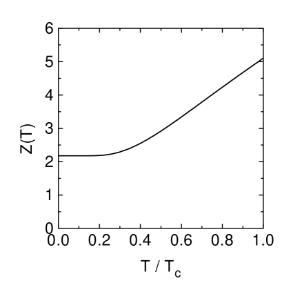
FIG. 5.: The function $Z(T)$, Eq. (46), defining the temperature dependence of the ratio $\delta j(\Phi)/I(\Delta)$, Eq. (44).

Similarly, we can calculate by using Eqs. (40) and (41) the asymptotic values of the correction $\Delta_{1}(0)$ to the unperturbed value of the order parameter at the junction:

$${\Delta_{1}\over\Delta_{0}}\!\!=\!-\alpha(T)W_{0}\sin^{2}\!{\Phi\over 2},\;\alpha(0)\!=\!3.037,\;\alpha(T_{c})\!=\!5.782.$$ (56)

The dependence of the order parameter $\Delta(0)$ on the phase jump at the junction at $T=0$ presented in Fig. 1 shows that the main contribution to the energy gap suppression comes from the depairing mechanism considered in Sec. 3, and the change in the order parameter is smaller than the variation of $\epsilon_{\ast}(\Phi)$.

The structure of the phase and temperature dependences of the correction to the Josephson current of Eq. (44) in a diffusive superconductor virtually coincide with expression Eq. (1) for a junction between pure metals except the following circumstance noted in Introduction: the parameter of the expansion of $j(\Phi)$ in the transmissivity of the junction for $l\ll\xi_{0}$ is not the tunneling probability $\Gamma$, but a considerably larger parameter $W$, Eq. (5). This allows one to observe higher harmonics of the current–phase dependence in diffusive tunnel junction with a comparatively high resistance. Koops et al. [21] apparently reported on the first experimental results in this field.

The theory discussed above describes the current–phase dependence for a diffusive Josephson junction in the whole temperature range $0\leq T<T_{c}$ except a narrow neighborhood of $T_{c}$ in which $\Delta/T_{c}\sim W_{0}$ ($\Delta/T_{c}\sim\Gamma$ in a pure superconductor), and the magnitude of corrections Eqs. (44) and (1) becomes comparable with $j_{0}(\Phi)$, while the correction Eq. (48) to $\Delta$ becomes of the order of its unperturbed value. This means that in the definition Eq. (5) of the parameter $W$ near $T_{c}$ the coherence length $\xi_{0}(T)$ describing the characteristic scale of spatial variations of Green’s function and density of states should be replaced by the characteristic length $\xi(T)$ of variation of the order parameter (healing length) in the Ginzburg–Landau theory, whose order of magnitude is the same as $\xi_{0}$ far away from $T_{c}$. Taking into account the results of calculations of $j(\Phi)$ for a pure superconductor in the vicinity of $T_{c}$ [7], we can obtain the following interpolation estimate of the effective transmissivity $W$ suitable for any temperatures and mean free paths:

$$W\sim\Gamma\xi(T)\left({1\over l}+{1\over\xi(0)}\right).$$ (57)

As we approach $T_{c}$, the value of $W$ increases infinitely, which is accompanied with a decrease in the phase jump for a given external current bounded by its critical value. Thus, in the 1D geometry for an arbitrarily large normal resistance of the junction, there exists a narrow region near $T_{c}$ in which the phase difference of the order parameter at the junction is small up to values of current of the order of the bulk critical current.

The authors are grateful to T.N. Antsygina and V.S. Shumeiko for fruitful discussions.

This research was supported by the Foundation for Fundamental Studies at the National Academy of Sciences of the Ukraine (grant No. 2.4/136).

REFERENCES

[1]
N. van der Post, E.T. Peters, I.K. Yanson, and J.M. van Ruitenbeek, Phys. Rev.
Lett. 73, 2611 (1994).
[2]
H. Takayanagi, T. Akazaki, and J. Nitta, Phys. Rev. Lett. 75, 3533
(1995).
[3]
W. Haberkorn, H. Knauer, and S. Richter, Phys. Status Solidi 47, K161
(1978); A.V. Zaitsev, Sov. Phys.–JETP 59, 1015 (1984); G.B. Arnold,
J. Low Temp. Phys. 59, 143 (1985).
[4]
The transverse size of the junction is assumed to be smaller than the
Josephson penetration depth, which ensures the uniform distribution of the
current over the cross section of the junction.
[6]
The only exception is the case of temperatures close to critical, when the
presence of the small parameter makes it possible to formulate
the effective computational algorithm of the solution of this problem
[7, 8].
[11]
V. Ambegaokar and A. Baratoff, Phys. Rev. Lett. 10, 486 (1963).
[12]
Strictly speaking, this relation contains the jump in the phase of Green’s
function instead of the jump in the order parameter phase, but these
quantities virtually coincide for (see Sec. 4).
[13]
A. Furusaki and M. Tsukada, Phys. Rev. B43, 10164 (1991).
[14]
S.V. Kuplevakhskii and I.I. Fal’ko, Sov. J. Low Temp. Phys. 17, 501
(1991).
[16]
Yu.V. Nazarov, Phys. Rev. Lett. 73, 1420 (1994).
[17]
N. Argaman, cond-mat/9709001 (1997).
[18]
The concept of adiabatic deformation of “energy levels” in the continuous
spectrum of a superconducting diffusive system in the current-carrying state
and their classification on the basis of the continuous “quantum number”
was introduced for the first time in Ref. [19] and systematically
used in Ref. [20].