A 2-D asymmetric exclusion model for granular flows

I Introduction

Among the numerous problems dealing with granular materials, one of the most challenging is granular sheared flow[1, 2, 3]. Thus, although granular materials might exhibit solid, liquid or gas-like properties[1], the granular flows cannot be described simply. Granular sheared flow arises in many different contexts such as pipe flow, pyroclastic flows[4], or even traffic jams[5]. Experiments performed in 2-D and 3-D geometries show surprising velocity profiles. First, the flow occurs only in a sheared region whose width is typically on the order of ten particle sizes (the shear zone). Also, velocity profiles appear to behave differently in 2 and 3 spatial dimensions. The velocity decreases exponentially with the distance to the wall in 2-D with a small Gaussian correction[6], while in 3-D the profile is almost purely Gaussian[7]. The goal of this paper is to present a two dimensional “toy model” where the velocity profile evolves correspondingly from an exponential like form to an almost Gaussian form. The model consists of vertically coupled layers. Each layer follows the well known asymmetric exclusion (ASEP) model. In one dimension, the ASEP model has been widely studied and under certain conditions, exact solutions have been found using the infinite dimension matrix method[8]. However, to our knowledge, very little is known concerning 2-D ASEP model. Our numerical simulations will in fact show a cross-over between an exponential velocity profile and a Gaussian velocity profiles when the control parameter crosses the value $1/2$. This could be interpreted as a phase transition in infinite size systems, as the study of the clusters size distribution will indicate. Finally a mean field approach will be developed for the low values of the control parameter.

II The model

The 1-D ASEP model with periodic boundary conditions describes a one-dimensional lattice of N sites, where each site $i$ ($1\leq i\leq N$) is either occupied by a particle or empty. During time interval $dt$, each particle has a probability $dt$ of jumping to the adjacent site to its right if that site is empty. Our 2-D has a simplified dynamics since the time is now discretized ($t_{n}=n$). Each layer is a one dimensional lattice of $N$ sites, with periodic boundary conditions. The layers are labeled $L_{k}$ ($k\geq 0$). Each site is either occupied or empty and the density along each layer is set to be constant ($=\rho$). A shift of one half of the grid spacing is applied between consecutive layers, so that for $k$ even $i$ is an integer and for $k$ odd, $i$ is an half integer (see figure 1). The 2-D lattice is composed of an infinite number of layers occupying the half space $y\geq 0$. At time $t_{n}$, each particle has a probability $P_{i,k}(t_{n})$ of hoping to the right. The quantity $P_{i,k}(t_{n})$ is determined by the dynamics of the four nearest neighbors of the site $(i,k)$: two in the row $L_{k-1}$ at time $t_{n}$ and two in the row $L_{k+1}$ at time $t_{n-1}$. $P_{i,k}(t_{n})$ is simply proportional to the number of these neighbors that are moving with a proportionality coefficient $\alpha$. In addition, the exclusion principle imposes that the particle cannot jump to an occupied site. However, if the particle on site $(i+1,k)$ is jumping to its right at time $t_{n}$ then the particle on site $(i,k)$ is allowed to move. If $Q_{i,k}(t)$ is the characteristic function of the motion for the site $(i,k)$ at time $t$ ($Q_{i,k}(t)=1$ if there is a particle at time $t$ that is jumping from site $(i,k)$, and is zero otherwise) the equation for $P_{i,k}(t_{n})$ reads:

$$P_{i,k}(t_{n})=\alpha(Q_{i-1/2,k-1}(t_{n})+Q_{i+1/2,k-1}(t_{n})+Q_{i-1/2,k+1}(t_{n-1})+Q_{i+1/2,k+1}(t_{n-1}))$$ (1)

For consistency, if the right hand side of the formula (1) is bigger than $1$ then we define $P_{i,k}(t_{n})=1$. Eventually, our boundary condition will represent a moving wall situated at $k=-1$: all the sites of $L_{-1}$ are filled and are moving at each time step. No boundary condition is required for $k=\infty$. The velocity $V_{k}(t_{n})$ is defined as the probability that a particle located on row $L_{k}$ moves at time $t_{n}$. Then, the mean value of the velocity on row $L_{k}$ is denoted $V(k)$ and defines the velocity profile.

The only control parameter of the dynamics is $\alpha$. Experimental observations suggest that $\rho$ should be taken close to $1$. It appears from the simulations that the dependence on $\rho$ is trivial, and we consider results for $\rho=0.9$. On the other hand, $\alpha$ reveals how much a moving particle pushes on its neighbors. Therefore, it has to be a (non trivial a priori) function of the material properties such as the friction, the shape of the grains, their roughness, etc…

The model does not allow exchange of particles from one row to another (along the $y$ direction). This strong constraint is in opposition with the experimental observations, where the density profile seems to reach a steady state where the exchanges between rows just balance. We assume in fact in this model that this interchange of particles is not relevant compared to the friction effects. We also checked that by imposing a reasonable density profile from the moving boundary to the bulk, the qualitative results of the model are not affected.

III Numerical results.

Figure (2) shows different velocity profiles for $\rho=0.9$ and $\alpha$ increasing from $0.2$ to $0.65$. For $\alpha\geq 1/2$, an abrupt change in the velocity profile is observed. In fact, we can expand the logarithm of the velocity in a Taylor serie:

$$ln(V(k))=a+b\cdot k+c\cdot k^{2}+d\cdot k^{3}...$$ (2)

We remark that the three first terms on the right hand side of (2) give a qualitatively good approximation of the velocity profiles. It correspond to a Gaussian fit of the profile. However, the ratio $b/c$ indicates the typical width for which the quadratic term becomes of the same order as the linear one. For $\alpha<0.5$ this ratio is of order of hundreds, i.e. much larger than the shear width and the dynamics can be considered almost purely exponential. On the other hand, the ratio $b/c$ becomes of the order of $1$ when $\alpha$ crosses the critical value $\alpha_{c}=0.5$, so that one can approximate the velocity profiles for $\alpha>\alpha_{c}$ with a Gaussian centered near the row $k=0$. Such property appears clearly on the insert of figure (2), where the velocity profile for $\alpha=0.65$ as a function of $k^{2}$ is shown. Notice that for small $k$ ($k^{2}<500$), the logarithm of the velocity is almost linear in $k^{2}$, so that one can consider that the velocity profile is Gaussian at least near the wall.

The instantaneous velocity $V_{k}(t)$ shows also different behaviors wether $\alpha$ is larger or smaller than $\alpha_{c}$. Thus, for $\alpha\geq 0.5$, transitory dynamics occur for small time ($t_{n}<100$) until the velocity reaches a stationary behavior. Such transitory states cannot be seen for $\alpha$ smaller than $0.5$.

In order to investigate more carefully the transition occurring at $\alpha=\alpha_{c}$, as well as the velocity profiles, a simplified version of the model is introduced. It exhibits the same properties as the model explained above, and can be more easily studied analytically. It consists of neglecting the effect of the row $L_{k+1}$ on the dynamics in row $L_{k}$. The model breaks the symmetry along the $y$ direction. However, experimentally, the sheared flows exhibit a spontaneous symmetry breaking as well. A transition from exponential to Gaussian velocity profile occurs in the same way for this simplified model at $\alpha=\alpha_{c}$. Notice that $\alpha_{c}$ corresponds to the value of $\alpha$ at which the probability becomes $1$ to move if the two neighbors above are moving (the exclusion condition still holds).

We define $P(n)$ as the probability that, given a hole, the next hole on its right is located after $n$ filled sites. $P(n)$ gives the probability distribution function (PDF) for the size of the clusters (if two consecutive sites are empty, it is considered as a cluster of size $0$). A priori, the function $P(n)$ depends on $\rho$, $\alpha$ and the row number $k$. However, if we consider that the particles are placed randomly on the sites with a density $\rho$ (as do the initial conditions), one obtains the Poisson distribution $P_{0}(n)=(1-\rho)\rho^{n}$. As shown on figure (3), for $\alpha<\alpha_{c}$, $P(n)$ corresponds almost exactly to $P_{0}(n)$ for any $k$ and $\alpha$. Therefore, at each time step, the particles are distributed on the sites as if they were randomly placed with density $\rho$. On the other hand, for $\alpha\geq\alpha_{c}$, the function $P(n)$ differs from $P_{0}(n)$ in that the small size clusters are more frequent, while large clusters follow a Poisson-like law. In this case, $P(n)$ does not vary as $\alpha$ increases for a given row, but changes as the row number increases: the bigger $k$, the closer $P(n)$ approaches $P_{0}(n)$.

When $\alpha$ approaches $\alpha_{c}$ the PDF differs slightly from $P_{0}(n)$, so for $k=1$ we can expand $P(n)$ in the form (see insert of figure 3):

$$P(n)=a\delta_{n,0}+(1-a)\rho_{eff}^{n}(1-\rho_{eff}),$$

with $\rho_{eff}=\rho/(1-a(1-\rho))$ (mean density has to be $\rho$). Figure (4) shows the evolution of $a$ as a function of $\alpha$ for $\rho=0.9$. For $\alpha>\alpha_{c}$, $a$ is a constant since $a=a_{c}=0.25\pm 0.01$ which corresponds to $\rho_{eff}\sim 0.92$. However, for $\alpha\leq\alpha_{c}$ we observe that for $a\sim a_{c}$:

$$a_{c}-a\propto(\alpha_{c}-\alpha)^{\nu}$$

and we found $\nu\sim 2/3$. Therefore, we identify the behavior of the system when $\alpha$ reaches $\alpha_{c}$ as a phase transition. Notice that when $\alpha$ increases above $\alpha_{c}$, the PDF shows a more complex behavior since not only the value of $P(0)$ is disturbed, but also a larger range of small clusters size $n$ (see figure 3).

IV Mean field theory

As the correlations can be neglected for $\alpha<\alpha_{c}$, a mean field approach is appliable. Defining $P^{(k)}(n)$ as the probability that $n$ successive particles are moving on the row $L_{k}$ (knowing that an empty site is before such a cluster), $P^{(0)}(n)$ can be computed exactly: $P^{(0)}(n)=(2\alpha\rho)^{n}(1-2\alpha\rho)$ and by noticing that $V(0)=\frac{(1-\rho)}{\rho}\sum nP^{(0)}(n)$, we obtain:

$$V(0)=\frac{2\alpha(1-\rho)}{1-2\alpha\rho}$$

It is remarkable that the numerical simulations and this mean–field solution agree within an error of less than one percent. Also, one can write the constitutive relation between $P^{(0)}$ and $P^{(1)}$:

$$P^{(1)}(n)=\sum_{l=n-1}^{\infty}W(l\rightarrow n)P^{(0)}(l)$$ (3)

where $W(l\rightarrow n)$ is the probability that if a cluster of size $l$ at row $k=0$ is moving, then a cluster of size $n$ at row $k=1$ is moving. It follows that:

$$W(l\rightarrow n)=(1-\rho)(2\alpha\rho)^{n}\left((l-n+1)-(l-n)2\alpha\rho\right)\quad{\rm for}\quad l>n$$

$$W(n\rightarrow n)=(1-\rho)\alpha\rho(2\alpha\rho)^{n-1}(2-\alpha\rho);W(n-1\rightarrow n)=(1-\rho)(\alpha\rho)^{2}(2\alpha\rho)^{n-2}$$

and we obtain for $V(1)$:

$$V(1)=\frac{1-\rho}{\rho}\sum_{n=1}^{\infty}nP^{(1)}(n)=\frac{2\alpha^{2}\rho(1-\rho)^{2}(2+\alpha\rho(1-2\alpha\rho)^{2})}{(1-2\alpha\rho)^{2}(1+2\alpha\rho)}.$$

Again, this mean–field solution is in good agreement with the numerical results, although not as accurate than for $V(0)$. Unfortunately, the next order step, for obtaining the analytical solutions of $P^{(1)}$ and then $V(2)$ are much more complicate. However, one can consider that for the exponential behavior, the knowledge of $V(0)$ and $V(1)$ is sufficient. Then, we can compare the numerical exponential profile with the exponential law predicted by the mean–field. We define $r(\alpha,\rho)$ such that for $\alpha<\alpha_{c}$, the velocity profile obtained numerically is fit by: $V(k)=V(0)(r(\alpha,\rho))^{k}$

Figure (5) shows $log(r)$ as function of $\alpha$ for $\rho=0.9$, compared with the mean–field $r_{mf}$ solution taken as:

$$r_{mf}=\frac{V(1)}{V(0)}=\frac{\alpha\rho(1-\rho)(2+\alpha\rho(1-2\alpha\rho)^{2})}{1-(2\alpha\rho)^{2}}$$

Thus, the mean–field approximation, deducing the exponential law from the ratio between the two first velocities, gives a quantitative good approximation of the exponential decay for $\alpha<\alpha_{c}$.

But, for $\alpha\geq\alpha_{c}$, the mean–field approach fails and we are not able to show analytical results. Although we were able to quantify the coorelations for $\alpha\sim\alpha_{c}$, numerical simulations show correlations along the $y$ direction as well. However, we believe that the phase transition exhibited by the model might have interesting features in granular flows. Particularly, it might be interesting to perform an experiment where the friction coefficient of the granular materials would change. Also, the model shows a phase transition between exponential and Gaussain behavior as $\alpha$ increases, while experimentally, the different behaviors occur between 2 and 3 spatial dimensions. In fact, one can imagine, for example, that the 3-D experiment can be linked to this 2-D ASEP model with an effective friction coefficient $\alpha_{3D}$. Then, if one consider that in 3-D each particle has more neighbors that can push it, it is plausible to assume that $\alpha_{3D}>\alpha_{2D}$ and possibly $\alpha_{3D}>\alpha_{c}\alpha_{2D}$ under certain conditions. Also, we would like to point out other applications of this model such as non-newtonian flows or molecular frictions.

Finally, notice that he model is based mainly on probabilistic properties of granular flows. Other stochastic approaches have already been proposed in this context[9, 10], although in granular materials there is no justification such as thermal fluctuations for stochastic processes. However, the shape of the grains, and therefore the contact network in granular materials can be considered as random variables (this has been argued for the chain forces in static bead pile[11]). Additionally, the motion of the particles in shear flows changes the configuration of the contact network of the system.

It is my pleasure to thank Eli Ben-Naim, Dan Mueth, Georges Debregeas and Leo Kadanoff for their advice and their interest on this work. I also acknowledge the ONR (grant: N00014-96-1-0127), the MRSEC with the National Science Foundation DMR grant: 9400379 and the ASCI Flash Center at the University of Chicago under DOE contract B341495 for their support.

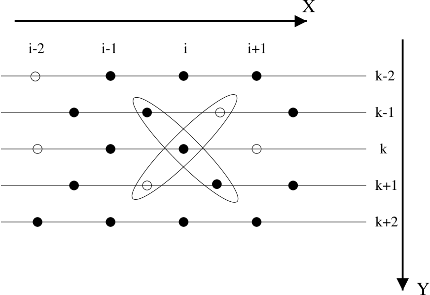
FIG. 1.: 2-D lattice with sites (circle) at time $t_{n}$: the white circles represent the empty sites or holes, while the black circles represent particles. The motion of the particle located at the position $(i,k)$ is determined as indicated by the motion of its four closest neighbors on rows $L_{k+1}$ and $L_{k-1}$.

FIG. 2.: Velocity profile for a density $\rho=0.9$ for different values of the control parameter $\alpha$. $\alpha$ increases from $0.2$ to $0.65$ in increments of $0.05$ as the curves are plotted from the left to the right. For $\alpha$ smaller than one half the profile is almost exponential and it is far from exponential for $\alpha\geq 0.5$. The insert shows the velocity profile for $\alpha=0.65$ as a function of $k^{2}$. It shows that the profile is better approximated by a Gaussian law, particularly for the low values of $k$. The number of sites per row is $20000$ and the average is computed over $4000$ time iterations for $5$ different initial conditions for each $\alpha$.

FIG. 3.: The probability distribution function of the cluster size for different values of $\alpha$ and $k$, and for $\rho=0.9$. The straight line corresponds to $P_{0}(n)$ and is $P(n)$ for $\alpha=0.45$ and $k=1$. The two others PDF shown are for value of $\alpha$ larger than $\alpha_{c}$. The one that is maximum for $n=0$ is for $\alpha=0.5$ and $k=1$ while the nest highest is for $\alpha=0.6$ and $k=4$. Notice that they show Poisson-like tails at large $n$, with different slopes. Insert: for $\alpha=0.49$ and $k=1$, the PDF differs from $P_{0}(n)$ only at $n=0$.

FIG. 4.: The density of holes $a$ as a function of $\alpha$ near the phase transition ($\alpha=\alpha_{c}=0.5$). $a$ is approximately constant for $\alpha>\alpha_{c}$ and exhibits a critical exponent of $2/3$ for $\alpha\leq\alpha_{c}$.

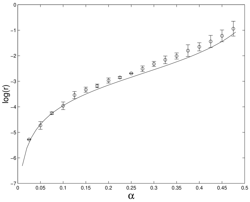
FIG. 5.: $log(r(\rho,\alpha))$ obtained by numerical simulation (circles) for $\rho=0.9$ compared to the mean–field approximation $log(V(1)/V(0))$ (line). $log(r)$ is computed by a Gaussian fit of the numerical results. The error bars have been evaluated by comparing it with an exponential fit.

REFERENCES

- [1] H. Jaeger, S. Nagel and R. Behringer, Rev. Mod. Phys. 68, 1259 (1996).
- [2] J. Rajchenbach, in Physics of Dry Granular Media, NATO ASI Series E350, 421 (1998).
- [3] L. Kadanoff, Rev. Mod. Phys. 71, 435 (1999).
- [4] S. Straub, Geol. Rundsch. 85, 85 (1996).
- [5] E. Ben-Naim, P.L. Krapivsky and S. Redner, Phys. Rev. E 50, 822 (1994)
- [6] C. Veje, D. Howell, R. Behringer, S. Schöllmann, S. Luding and H. Herrmann, in Physics of Dry Granular Media, NATO ASI Series E350, 237 (1998); C.T. Veje, D.W, Howell and R.P. Behringer, Phys. Rev. E 59, 739 (1999).
- [7] D. M. Mueth, G. F. Debregeas, G. Karczmar, H. M. Jaeger and S.R. Nagel, preprint (1999).
- [8] B. Derrida, M. Evans, V. Hakim and V. Pasquier, J. Phys. A: Math. Gen 26, 1493 (1993).
- [9] O. Pouliquen and R. Gutfraind, Phys. Rev. E 53, 552 (1996).
- [10] G. Debregeas and C. josserand, cond-mat/9901336.
- [11] C. Liu, S. Nagel, D. Schecter, S. Coppersmith, S. Majumdar, O. Narayan and T. Witten, Science 269, 513 (1995); D.M. Mueth, H.M. Jaeger and S.R. Nagel, Phys. Rev. E 57, 3164 (1998)