[

Triangular anisotropies in Driven Diffusive Systems: reconciliation of Up and Down

Abstract

Deterministic coarse-grained descriptions of driven diffusive systems (DDS) have been hampered by apparent inconsistencies with kinetic Ising models of DDS. In the evolution towards the driven steady-state, “triangular” anisotropies in the two systems point in opposite directions with respect to the drive field. We show that this is non-universal behavior in the sense that the triangular anisotropy “flips” with local modifications of the Ising interactions. The sign and magnitude of the triangular anisotropy also vary with temperature. We have also flipped the anisotropy of coarse-grained models, though not yet at the latest stages of evolution. Our results illustrate the comparison of deterministic coarse-grained and stochastic Ising DDS studies to identify universal phenomena in driven systems. Coarse-grained systems are particularly attractive in terms of analysis and computational efficiency.

]

Driven steady-state systems are common in many fields of physics including device physics and materials processing, and are also found in many biological processes. The simplest example of a driven system is one in which a uniform external drive is applied. For closed boundary conditions, a final equilibrium state is reached in which the external drive is balanced by other forces — as in a closed system in a gravitational field. For open boundaries, equilibrium will never be reached and a non-equilibrium steady state will continue “indefinitely”. Electrical circuits provide prosaic examples of this. In both open and closed systems, the introduction of local interactions provide a rich phenomenology that is only slowly being explored.

To model a driven system we must describe both the energetics and the dynamics. One of the simplest such model is a lattice driven diffusive system (DDS). This is simply an interacting lattice gas with biased motion in the direction of the uniform external field. Early work on this model concentrated on steady-state properties near the critical point, which survives from the underlying zero-field Ising model. More recently there has been increasing emphasis on the approach to the steady state. This dynamical regime is independent of the open or closed boundary conditions, and hence is common to both. See the book by Schmittmann and Zia [1] for an introduction to the literature.

One of the most important questions we can ask about any model is whether the behavior that it displays is universal. To whit: is the observed behavior seen in a broad class of systems, or is it specific to that precise model? For example, we can ask whether a lattice DDS and related coarse-grained models display the same universal behavior. This question has proven remarkably controversial in DDS, and this paper aims towards a reconciliation between lattice and coarse-grained approaches.

Near the critical point separating the low-temperature ordered and high-temperature disordered DDS phases, coarse-grained descriptions lead to analytic solutions of the steady-state structure [2]. Ising DDS simulations have been consistent with these results [3] on balance, though they have been performed mainly at infinite fields [4]. [There have been claims that different approaches, though still coarse-grained, should apply in that infinite-field limit [5, 6].] Away from the critical point, the focus has been on the approach towards the final steady state and the question has been whether any coarse-grained model recovers the phenomenology of a stochastic Ising DDS. In the ordered steady-state of both the lattice gas and related continuum descriptions, the domain walls align with the field direction and fluctuations are suppressed to a remarkable degree [1]. The main difference occurs in the approach to the steady-state, and is easiest to visualize in a system with a marked minority of one of the ordered phases (so-called “off-critical” systems). There, separated droplets nucleate and diffusively coarsens [for the zero-field limit see [7]]. As the drops grow, they elongate in the field direction — ultimately forming the stripes of the steady-state. This phenomena is seen both in the lattice DDS [8] and in continuum models [9]. However, the drop shapes are triangular and point in opposite directions with respect to the field in the Ising and coarse-grained models (see, however, [10]). As seen in Fig. 1, the tips of the triangles point against the field direction (up) in the lattice model, while they point with the field (down) in the continuum simulations. The same triangular anisotropy, and discrepancy, is seen at other volume fractions as well.

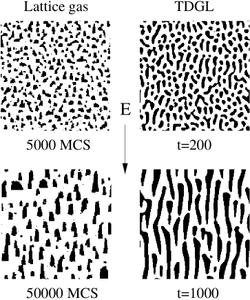
FIG. 1.: Evolution of domains for an off-critical quench in a lattice gas with nearest neighbor hops (left) and for a TDGL coarse-grained model with isotropic mobility (right). The field ${\bf E}$ biases the motion of the particles (dark) downwards. For the lattice gas the tips of the triangular domains point “up”, opposite the field, for the coarse-grained model the domains point “down”.

Does this indicate that either the Ising DDS models, or the coarse-grained models (or both!) are non-universal? Either would be less than ideal, since stochastic (Ising) models are needed for temperature-dependent studies near the critical point, and deterministic coarse-grained models are both analytically tractable and more computationally efficient at lower temperatures. An attractive resolution would be that there are regimes of parameter space in both stochastic Ising and deterministic coarse-grained models which exhibit either sign of triangular anisotropy, down or up with respect to the field, with the previously studied models being in the two different regimes. We take that as a working assumption, and try to flip the anisotropy by varying model parameters in the Ising and coarse-grained approaches. We report partial success, with asymptotic reversal in the Ising DDS and reversal up to intermediate times in the coarse-grained DDS, and we have by no means exhausted the phase-space of model parameters.

Even if we achieve full success, fundamental questions remain. Is the triangular anisotropy simply a non-universal amplitude, or does it lead to different phenomenology? How do we understand the temperature and field dependence of the anisotropy, and how does the observed anisotropy in the dynamic correlations reflect anisotropies due to the surface tension, particle mobility, and the external field? Reconciling the Ising and coarse-grained approaches is simply the start of the story.

Lattice Gas Dynamics

The basic discrete DDS model [1, 3, 8] is an extension of an Ising model with conserved Metropolis dynamics: particles hop with probability

$$W=Min\left[1,\exp\left(-\beta\Delta H\right)\right],$$ (1)

where the energy difference $\Delta H=\Delta H_{\rm Ising}+\Delta H_{\rm Field}$ includes an applied field. Restricting ourselves to a two-dimensional square lattice, $\Delta H_{\rm Ising}$ is the standard nearest neighbor Ising Hamiltonian in which a particle interacts with its four nearest sites. [We absorb $J/k_{B}$ into the temperature, which we then measure with respect to the zero-field Ising $T_{c}$.] $\Delta H_{\rm Field}$ is $+E$ if the particle moves one lattice unit opposite the field direction and $-E$ if the particle moves in the field direction, where $E$ is the field strength. The dynamics are conserved, so particles hop rather than being created nor destroyed. Restricting the hops to nearest neighboring sites, Alexander et al. [8] found that the domains formed upward pointing triangles, as shown in Fig. 1.

Natural generalizations of this well studied DDS model include looking at different lattices [triangular, hexagonal, and Kagomé in $2d$], rotating the field away from a lattice direction [11], allowing hops and/or interactions with further neighbor particles, and allowing anisotropic hop rates and interactions. Universal results on the basic model should be robust to these sorts of microscopic differences, as differences will certainly be entailed by experimental realizations. [These changes will affect variously the anisotropic particle mobility and interfacial surface tension of any coarse-grained representation.] In this paper we allow next-nearest-neighbor hops, where we treat all eight immediate neighbors with equal weight. We label these “nnn” dynamics, in contrast to “nn” dynamics where hops are restricted to the four nearest-neighbors.

Coarse-grained Dynamics

The simplest coarse-grained dynamics is the time-dependent Ginzburg-Landau (TDGL) model with a field. The free energy is given as

$$F[{\phi}] = \int dr\left[f(\phi(r))+\frac{1}{2}|\nabla\phi|^{2}+Ez\phi\right],$$ (2)

where $\phi({\bf r},t)$ is the order parameter and the field ${\bf E}$ points down toward lower $z$. Within a uniform phase, we use the following Flory-Huggins type free-energy density:

$$f(\phi)=(1+\phi)\ln(1+\phi)+(1-\phi)\ln(1-\phi)-\frac{a}{2}\phi^{2}.$$

The system will phase separate for $a>2$ with coexistence values depending on $a$. [For $a\approx 2$ this recovers a more familiar $\phi^{4}$ free energy.] This choice of $f(\phi)$ forces $|\phi|<1$, which simplifies the treatment of the particle mobility (below).

We choose standard TDGL dynamics driven by gradients in the chemical potential, so that the particle current is

$$\vec{J} = -M(\phi)\nabla\frac{\delta F}{\delta\phi},$$ (3)

where $M(\phi)$ is an order parameter dependent mobility. A continuity equation is then used to determine the evolution of the order parameter:

$$\frac{\partial\phi}{\partial t} = -\nabla\cdot\vec{J}$$ (4)

$$= \nabla\cdot M(\phi)\left(\frac{df}{d\phi}-\nabla^{2}\phi\right)+E\frac{\partial M(\phi)}{\partial z}.$$ (5)

The choice of a constant mobility $M(\phi)=M_{0}$ leads to the field dependence dropping out of the dynamics. The next simplest choice, $M(\phi)=M_{0}(1-\phi^{2})$, the exact mobility for non-interacting lattice-gases, leads to a non-trivial field-dependent DDS coarsening [8, 12, 13]. Indeed, because the dynamics are deterministic, a semi-quantitative understanding can then be reached for the linear stability of interfaces and other interfacial properties [9]. More generally, we want the mobility to reflect the effective coarse-grained mobility. Starting from a stochastic model with an applied field, the coarse-grained mobility will generally be anisotropic, as can be seen explicitly near the critical point [2]. As a minimal step, we allow for different mobilities for currents in the $x$ and $z$ directions with

$$M_{x}(\phi) = (1+m)M_{o}(1-\phi^{2}),$$ (6)

$$M_{z}(\phi) = M_{o}(1-\phi^{2}),$$ (7)

where $m$ describes the mobility enhancement transverse to the field direction [14]. In the simulations presented here we take $a\approx 2.75$, so that the bulk phases are at $\phi=\pm 0.8$. We always set $M_{0}=1$, which fixes the overall timescale. The initial conditions $\phi({\bf r},0)$ follows a Gaussian distribution around $\langle\phi\rangle$.

Asymmetry Measure

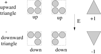
FIG. 2.: The normalized asymmetry measure is $asym=(n_{up}-n_{down})/(n_{up}+n_{down})$, where the configurations on top contribute to $n_{up}$ and those below contribute to $n_{down}$.

In order to quantitatively compare the models, we need a measure of triangular anisotropy. We use the microscopic measure shown in Fig. 2. That is, we examine all squares of four nearest-neighbor sites on our lattice and define $n_{up}$ as the number of squares in which the bottom two sites are positive but the top two sites have opposite signs. These configurations point “upward”. A similar definition is used for $n_{down}$. The normalized asymmetry measure is then

$$asym=\frac{n_{up}-n_{down}}{n_{up}+n_{down}},$$ (8)

so that $asym=1$ if all triangles are upward pointing and $asym=-1$ if all triangles are downward pointing. Squares with more or less than three filled sites are not counted. The same measure is used for the continuum model except we look at four neighboring mesh points and count ‘full’ and ‘empty’ as $\phi>0$ and $\phi<0$, respectively. [In practice an equivalent asymmetry measure for the ‘empty’ phase can be constructed. Similar results are obtained.] Our measure is quantitatively different from that of Alexander et al [8] where normalization drives their asymmetry towards zero as domains grow larger, however we obtain the same qualitative sign of the triangular asymmetry. We prefer our measure since it only depends on the shapes of triangles and not their size, at least in the coarse-grained formulation. It qualitatively agrees with anisotropies seen “by eye”.

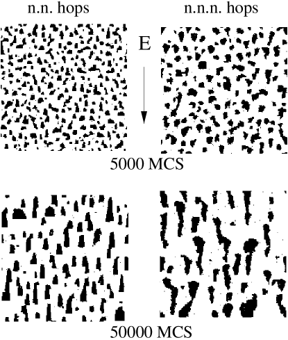
FIG. 3.: Configuration snapshots of the Ising DDS with nn (nearest neighbor) and nnn (next nearest neighbor) hops. The triangles point in opposite directions with respect to the field. In both cases, $\beta E=0.5$ and $T=0.5T_{c}$.

Lattice Gas Results

FIG. 4.: The asymmetry measure as a function of time for the Ising model with nn and nnn hops, where $\beta E=0.5$. The measure seems to approach an asymptotic value.

By including next nearest neighbor jumps we can flip the direction of the triangular domains with respect to the field. Fig. 3 illustrates our results for the Ising model with nn and nnn hops. This indicates that the sign of the triangular anisotropy is non-universal. We also observe that the evolution is more rapid when nnn hops are allowed, as probed by domain size.

The quantitative evolution of the asymmetry as a function of time for both nn and nnn hops is shown in Fig. 4. The data is averaged over 5 to 10 configurations to reduce the noise. The asymmetry starts small and eventually saturates to an asymptotic value. We cannot rule out further change [indeed slight decay is evident for $T=0.75T_{c}$] since there is no known dynamical scaling in the correlations, i.e. no time-independent scaling function.

The asymptotic asymmetry vs. $T/T_{c}$, where $T_{c}\equiv T_{c}(0)$ is the critical temperature for zero field, is shown in Fig. 5. With only nn hops the asymmetry is always positive, indicating upward pointing triangles, and increases with decreasing temperature. We note that the anisotropy measure is continuous across $T_{c}(E)$ (which ranges from $T_{c}(0)$ to approximately $1.4T_{c}(0)$ at $E=\infty$ [3]). At $T_{c}(E)$ we would expect surface tensions and particle mobilities to be isotropic in a small field, and so we attribute the residual anisotropy to the field. [We note that long-range correlations can persist into the high-temperature disordered phase due to violations in detailed balance in driven systems [1].]

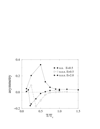
FIG. 5.: The asymptotic asymmetry vs. temperature for the Ising model. The nn model asymmetry is always positive, while the nnn model asymmetry is positive near the critical temperature and at the lowest temperatures. Some field dependence is also shown.

With nnn hops, the triangular asymmetry is small and positive near the critical point. This is consistent with the previous discussion of nn hops. At lower temperatures the asymmetry turns negative. Since the nnn hops should lead to a more isotropic particle mobility, we might infer that the increasing anisotropy of the surface tension with decreasing temperature feeds a negative triangular asymmetry when not sufficiently ‘compensated’ by an anisotropic mobility. Clearly the situation is complicated since to fully characterize the ‘anisotropy’ requires the entire function of, e.g., surface tension vs interfacial orientation. Without actually having a quantitative measure of the coarse-grained properties of the system (surface tension, particle mobility) it is difficult to discuss the exact origins of the triangular asymmetry. Indeed, this difficulty is a primary motivation to explore the coarse-grained picture. Regardless, the particle mobility will depend on the microscopic structure, which in turn depends on the applied field, even at $T=0$. In the limit of small applied field $E$ additional induced anisotropies should become negligible. We see some indications of this through the reduction in the low-temperature positive asymmetry regime with nnn hops as the field is reduced, indicating that the regime is induced by the finite field. This suggests one possible simplifying tactic: to look at the small field limit. Unfortunately this makes the timescales for numerical investigation of the driven system inaccessibly large. Analytically, this limit has been profitably used by one of us in a coarse-grained analysis of surface instabilities in nearly isotropic systems [9].

Coarse-grained Results

The results for the kinetic Ising model indicates that the positive asymmetry measure may be due to anisotropy in the mobility. Therefore to flip the triangles positive in the TDGL model, we allow for different mobilities in the the $x$ and $z$ (field) direction with $M_{x}/M_{z}=1+m$. We also varied the bulk coexistence value, the field strength $E$ and the initial filling fraction. We found that the primary effect came from $m$ and from $E$.

The top snapshot in Fig. 6 shows that the triangles are in the same direction as the n.n. kinetic Ising model at early times. This is confirmed by a positive asymmetry measurement at these times. However, the bottom snapshot in Fig. 6 shows that the asymmetry measure becomes negative at late times when the domains are very elongated in the field direction. This transient behaviour was robustly present at all nonzero values of m and E that we tried. However, the early time “transient” regime with positive asymmetry is quite large and can be extended indefinitely in the limit of $E/m\to 0$. This is shown in Fig. 7 which shows the asymmetry vs. time for critical quenches at fixed $m=1$ and varying $E$. This raises the intruiging question of whether the asymmetries seen in the Ising DDS models, where the underlying dynamics are slower, might switch at later times.

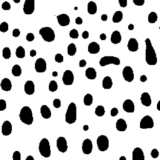
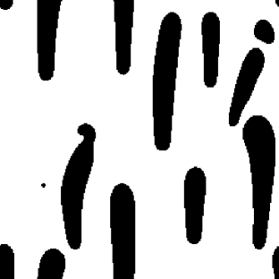
FIG. 6.: Configuration snapshots at $t=1600$ and $t=12800$ of an evolving coarse-grained system with $m=1$ and $E=0.1$. The reversal of the asymmetry, while not dramatic, can be seen. The applied field is downward in both snapshots.

FIG. 7.: The asymmetry as a function of time for fixed mobility anisotropy, $m=1$ and different fields. The asymmetry starts positive but then becomes negative at late times. The time for which the asymmetry is positive is extended for smaller fields.

Conclusion

We have shown that the sign and magnitude of triangular anisotropies of growing domains are non-universal in both stochastic Ising and deterministic coarse-grained DDS models. Hence, we see no qualitative differences between these approaches with finite fields, and rather see great promise in using the strengths of each approach to explore DDS phenomenology.

Questions remain concerning the origins of the triangular anisotropy within a full anisotropic coarse-grained model. This must be understood to intelligently explore the parameter space of coarse-grained models. With this understanding, we might even profitably turn the tables and use the triangular anisotropy as a probe of interfacial properties.

We are not overly concerned with the apparent transient nature of the “flipped” anisotropy in the coarse-grained model, since even the stochastic Ising model has not yet been extensively enough studied to tell if the anisotropies hold asymptotically late. However, we will now focus our efforts on prolonging the reversal in coarse-grained models. This provides a motivation to more fully understand the origins of the triangular anisotropy. In the process we would like to develop a more intrinsically coarse-grained measure of anisotropy that can be used equally well in Ising and coarse-grained approaches. We expect that anisotropies in the Porod tail of the structure factor will be the most robust measure, since they directly probe the distribution of interfacial orientations.

- [1] B. Schmittmann and R. K. P. Zia, Statistical mechanics of driven diffusive systems, v. 17 in the series Phase Transitions and critical phenomena (Academic Press, London, 1995).
- [2] H. K. Janssen and B. Schmittmann, Z. Phys. B 64, 503 (1986); K.-t. Leung and J. Cardy, J. Stat. Phys. 44, 567 (1986); ibid 45, 1087 (1986).
- [3] In see K.-t. Leung, Phys. Rev. Lett 66, 453 (1991); J.-S. Wang, J. Stat. Phys. 82, 1409 (1996); in see K.-t. Leung and J.-S. Wang, cond-mat/9805285.
- [4] The infinite field, , limit in a lattice DDS is singular since no currents can point against the field. This constraint on the currents will then persist in any accurate coarse-grained representation, though the coarse-grained field must be finite to produce finite currents. We might expect some non-universal results from Ising DDS in this limit, both in critical phenomena and away from . Indeed, while simulations of critical phenomena with [3] are consistent with the coarse-grained field-theoretic results with a finite field, some debate remains [5, 6]. Our resolution is simple: we restrict ourselves to finite fields.
- [5] J. Marro, A. Achahbar, P. L. Garrido, and J. J. Alonso, Phys. Rev. E 53, 6038 (1996); see related response by K.-t. Leung and R. K. P. Zia, J. Stat. Phys. 83, 1219 (1996).
- [6] P. L. Garrido, F. de los Santos, and M. A. Muñoz, Phys. Rev. E 57, 752 (1998); F. de los Santos and P. L. Garrido, cond-mat/9805211.
- [7] I. M. Lifshitz and V. V. Slyozov, J. Phys. Chem. Solids 19, 35 (1961).
- [8] F. J. Alexander, C. A. Laberge, J. L. Lebowitz, and R. K. P. Zia, J. Stat. Phys. 82, 1133 (1996).
- [9] C. Yeung, J. L. Mozos, A. Hernández-Machado, and D. Jasnow, J. Stat. Phys. 70, 1149 (1993).
- [10] Larger fields, above around in our units, suppress the triangular anisotropy in both lattice and coarse-grained approaches (R. K. P. Zia, private communication). However, if the anisotropy is not strictly zero, questions about its sign remain.
- [11] By eye, rotating the field with respect to the lattice axes induces an anisotropy reversal.
- [12] K. Kitahara, Y. Oono, and D. Jasnow, Mod. Phys. Lett. B 6, 765 (1988).
- [13] C. Yeung, T. Rogers, A. Hernández-Machado, and D. Jasnow, J. Stat. Phys. 66, 1701 (1992).
- [14] We do not cover the entire phase-space of deterministic coarse-grained models. In general one requires a fully anisotropic surface-tension, which can be selected by higher-order gradients in Eqn. 2. One also can require a fully anisotropic particle mobility, rather the simple elliptical anisotropy of Eqn. 6, with more general order-parameter dependence as well.