The random magnetic flux problem in a quantum wire

I Introduction

The concepts of scaling [2, 3, 4] and of the renormalization group[5] have provided crucial insights into the localization properties of a quantum particle in a random but static environment.[6] Beyond a typical length scale depending on the microscopic details of the disorder, the localization problem can be described by an effective field theory that is uniquely specified by the dimensionality of space and the fundamental symmetries of the microscopic Hamiltonian.[7] Correspondingly, the disorder is said to belong to the orthogonal, unitary and symplectic ensembles, depending on whether time reversal symmetry and spin-orbit coupling are present or not.[7, 8, 9]

However, not all disordered systems belong to one of these three standard symmetry classes. One example is the Integer Quantum Hall Effect, for which the scaling theory in the unitary universality class cannot explain the observed jumps in the Hall resistance,[10] since it predicts that all states are localized in two-dimensions. Instead, a new scaling theory was proposed for the Integer Quantum Hall Effect, where, in addition to the longitudinal conductivity that controls the scaling flow in the unitary ensemble, the Hall conductivity appears as a second parameter.[11, 12]

In this paper we consider a different example. It is the so-called random flux model, which describes the localization properties of a particle moving in a plane perpendicular to a static magnetic field of random amplitude and vanishing mean.[13, 14, 15, 16, 17, 18, 19, 20, 21, 22, 23, 24, 25, 26, 27, 28, 29, 30, 31, 32, 33, 34, 35] In the literature, different points of view have been offered with regard to the localization properties and the appropriate symmetry class of the random flux problem. In Refs. [19, 20, 21, 22, 23, 24, 25] it has been claimed that, since the magnetic field has a vanishing mean, the only effect of the random magnetic field is to break time reversal invariance, and hence that the localization properties are those of the standard unitary symmetry class. On the other hand, Zhang and Arovas[28] have argued that this argument might be too naive and that a scaling theory closely related to that of the Kosterlitz-Thouless transition controls the localization properties of the random magnetic flux problem. They predicted that states are localized in the tails of the spectrum whereas close to the center of the band a line of critical points of the Kosterlitz-Thouless type is formed. Related point of views can be found in Refs. [26, 27, 28, 29, 30, 31, 32, 33]. Finally, it has been proposed in Ref. [34] that the random flux model shows critical behavior at the band center $\varepsilon=0$ only, whereas its localization properties are those of the unitary ensemble for energies $\varepsilon\neq 0$.

In the third scenario, the behavior at $\varepsilon=0$ is governed by an additional symmetry, the so-called chiral or particle-hole symmetry. The chiral symmetry can also be found in the related problem of a particle hopping on a lattice with random (real) hopping amplitudes.[36] In the one-dimensional version of this problem, it is well established that the ensemble-averaged density of states diverges at the band center $\varepsilon=0$[37, 38] and that the ensemble averaged conductance decays algebraically with the length $L$ of the system.[39] For comparison, in the unitary symmetry class, the density of states is continuous at $\varepsilon=0$,[40] while the conductance decays exponentially with $L$. (The one-dimensional random-hopping problem has been studied in many incarnations, cf. Refs. [41, 42, 43, 44, 45, 46, 47].) For two-dimensional systems, the effect of the chiral symmetry was studied by Gade and Wegner[48] (see also Refs. [49, 50, 51, 52, 53, 54, 55, 56, 57, 58, 59]). They argued that the presence of the chiral symmetry results in three new symmetry classes, called chiral orthogonal, chiral unitary, and chiral symplectic. For disordered systems with chiral unitary symmetry, all states are localized except at the singular energy $\varepsilon=0$ at which the average density of states diverges. The relevance of the chiral unitary symmetry class to the random flux problem was pointed out by Miller and Wang.[34] (Only the chiral unitary class is of relevance, since time-reversal symmetry is broken in the random flux model.)

For the two-dimensional random-flux problem, sufficiently accurate numerical data are notoriously hard to obtain. Although a consensus has emerged that states are localized in the tails of the spectrum, it is impossible to decide solely on the basis of numerical simulations whether states are truly delocalized upon approaching the center of the band, or only deceptively appear so as the localization length is much larger than the system sizes that are accessible to the current computers. Moreover, it is very easy to smear out a diverging density of states in a numerical simulation (compare Refs. [14, 23] and [35]). In short, no conclusion has been reached in the debate about the localization properties of the two-dimensional random flux problem.

Here, we focus on the simpler problem of the random flux problem on a lattice and in a quasi one-dimensional geometry of a (thick) quantum wire with weak disorder, and restrict our attention to transport properties, notably the conductance $g$. For a wire geometry, numerical simulations can be performed with very high accuracy, and very good statistics can be obtained. Moreover, precise theoretical predictions for the transport properties can be made, both for the unitary symmetry class, and for the chiral unitary symmetry class. The wire geometry allows us to quantitatively compare the analytical predictions for the various symmetry classes and the numerical simulations for the random flux model. This comparison shows that, away from the critical energy $\varepsilon=0$, the $L$-dependence of the average and variance of the conductance $g$ are those of the unitary ensemble. At the band center $\varepsilon=0$, $\langle g\rangle$ and $\mbox{var}\,g$ are given by the chiral unitary ensemble. Hence, we unambiguously show that in a quasi one-dimensional geometry, the localization properties of the random flux model are described by the third scenario above, in which the $\varepsilon=0$ is a special point, governed by a separate symmetry class. Although our theory is limited to a quasi one-dimensional geometry, it does show the importance of the chiral symmetry at the band center $\varepsilon=0$ and may thus contribute to the debate about the localization properties of the random flux problem in higher spatial dimensions.

This paper was motivated by two recent works. First, in a recent paper, one of the authors[35] computed $\langle g\rangle$ and $\mbox{var}\,g$ numerically for the random flux model in a wire geometry to a very high accuracy. While for nonzero energies $\varepsilon$, the result was found to agree with analytical calculations for the unitary symmetry class,[60, 61, 62] for $\varepsilon=0$ a clear difference with the unitary symmetry class was observed. Second, for the chiral symmetry classes, a scaling equation for the distribution of the transmission eigenvalues in a quasi one-dimensional geometry was derived and solved exactly in the chiral unitary case by Simons, Altland, and two of the authors.[63] This scaling equation is the chiral analogue of the so-called Dorokhov-Mello-Pereyra-Kumar (DMPK) equation,[64, 65, 66] which describes the three standard symmetry classes and was solved exactly in the unitary case by Beenakker and Rejaei.[67] However, for the chiral unitary case, analytical results for the $L$ dependence of $\langle g\rangle$ and $\mbox{var}\,g$ were lacking, so that a comparison between the theory and the numerical results of Ref. [35] was not possible. In the present work this gap is bridged.

In a wire geometry, the chiral unitary universality class undergoes a striking even-odd effect first noticed by Miller and Wang:[34, 68] The conductance $g$ decays exponentially with the length $L$ if the number of channels $N$ is even, while critical behavior is shown if $N$ is odd, even in the limit of large $N$ that we consider here. In the latter case, the average conductance $\langle g\rangle$ decays algebraically, while the conductance fluctuations are larger than the mean. We analyze how the even-odd effect follows from the exact solution of the Fokker-Planck equation of Ref. [63] and compare with numerical simulations of the random flux model.

We close the introduction by pointing out that the random flux problem is also relevant to some strongly correlated electronic systems. In both the Quantum Hall Effect at half-filling [69, 70] and high $T_{c}$ superconductivity,[71, 15] strong electronic correlations can be implemented by auxiliary gauge fields. In this context, the random flux problem captures the contributions from the static transverse gauge fields. Notice that the chiral symmetry is not required on physical grounds both for the Quantum Hall Effect at half-filling and for high $T_{c}$ superconductivity. Another area of applicability for our results is the passive advection of a scalar field [72, 34, 73] and non-Hermitean quantum mechanics.[74, 75, 76, 59, 63] Finally, the striking sensitivity of the localization properties in the random flux problem to the parity of the number $N$ of channels is remarkably similar to that of the low energy sector of a single antiferromagnetic spin-$N/2$ chain to the parity of $N$,[77] on the one hand, or to the sensitivity of the low energy sector of $N$ coupled antiferromagnetic spin-1/2 chains to the parity of $N$,[78] on the other hand.

The paper is organized as follows. The random flux problem in a wire geometry is defined in section II. The average and variance of the conductance are calculated analytically in section III. Analytical predictions are compared to the numerical simulations in section IV. We conclude in Sec. V.

II The random magnetic flux model

In the random flux model one considers a spinless electron on a rectangular lattice in the presence of a random magnetic field with vanishing mean. The magnetic field is perpendicular to the plane in which the electron moves. In this paper, we study the random flux model in a wire geometry and for weak disorder. This system is described by the Hamiltonian

$${\cal H}\,\psi_{m,j} = -t[\psi_{m+1,j}+\psi_{m-1,j}]$$ (3)

$$\mbox{}-t\,(1-\delta_{j,N})e^{i\theta_{m,j}}\psi_{m,j+1}$$

$$\mbox{}-t\,(1-\delta_{j,1})e^{-i\theta_{m,j-1}}\psi_{m,j-1},$$

where $\psi_{m,j}$ is the wavefunction at the lattice site $(m,j)$, labeled by the chain index $j=1,\ldots,N$ and by the column index $m$, see Fig. 1(a). The Peierls phases $\theta_{m,j}$ result from the flux $\Theta_{m,j}=\theta_{m+1,j}-\theta_{m,j}$ through the plaquette between the sites $(m,j)$, $(m+1,j)$, $(m+1,j+1)$, and $(m,j+1)$. (The flux $\Theta_{m,j}$ does not uniquely determine all the phases along all the bonds. We have used this freedom to choose the nonzero phases along the transverse bonds only.)

FIG. 1.: (a) Lattice with $N=3$ threaded by random magnetic fluxes $\Theta_{m,j}$ in the disordered region $0<m<M$. (b) Quantum wire with a disordered region of length $L=Ma$. Incoming amplitudes are $c^{L}_{\nu,+}$ and $c^{R}_{\nu^{\prime},-}$, whereas outgoing amplitudes are $c^{L}_{\nu,-}$ and $c^{R}_{\nu^{\prime},+}$, $\nu,\nu^{\prime}=1,\ldots,N$, in the left and right leads, respectively. In a quasi one-dimensional geometry, $M\gg N$.

We consider a system with Hamiltonian (3) where the phases $\Theta_{m,j}$ take random values in a disordered strip $0<m<M$ only, and are zero outside.[13] We assume that the disordered region is quasi one-dimensional, i.e., $M\gg N\gg 1$, corresponding to a thick quantum wire. In the disordered region, the Peierls phases $\theta_{m,j}$ are chosen at random in such a way that the magnetic flux $\Theta_{m,j}=\theta_{m+1,j}-\theta_{m,j}$ is uniformly distributed in $[-p\pi,p\pi]$ with $0<p\leq 1$. To be precise, with $\theta_{m,j}$ given, $\theta_{m+1,j}$ is chosen from the interval $[\theta_{m,j}-p\pi,\theta_{m,j}+p\pi]$ with uniform probability $1/2p\pi$. The parameter $p$ controls the strength of disorder. We assume weak disorder, i.e., $p\ll 1$.

The boundary conditions in the transverse directions that are implied by the Hamiltonian (3) are “open”, i.e., there are no bonds between the chains $j=1$ and $j=N$. In this case, ${\cal H}$ has a special discrete symmetry, called the particle-hole or chiral symmetry: Under the transformation $\psi_{m,j}\to(-1)^{m+j}\psi_{m,j}$, one has ${\cal H}\to-{\cal H}$. Hence, for each realization of the random magnetic flux, the chiral symmetry ensures that there exists an eigenstate of ${\cal H}$ with energy $-\varepsilon$ for each eigenstate of ${\cal H}$ with energy $+\varepsilon$. Note that the band center $\varepsilon=0$ is a special point. The chiral symmetry is broken by the addition of a random on-site potential to the Hamiltonian (3). Another way to break the chiral symmetry is to add bonds between the chains $j=1$ and $j=N$ and to impose periodic boundary conditions in the transverse direction for $N$ odd. The presence of the chiral symmetry may have dramatic consequences for charge transport through the disordered wire, as we shall see in more detail in the next sections.

In order to find the conductance $g$ of the disordered region with the random flux, we first compute the transfer matrix ${\cal M}$. To the left and to the right of the disordered region, the wavefunction $\psi_{m,j}$ that solves the Schrödinger equation ${\cal H}\psi=\varepsilon\psi$ can be written as a sum of plane waves moving to the right $(+)$ and to the left $(-)$,

$$\psi_{j,m} = \sum_{\nu=1}^{N_{c}}\sum_{\pm}c_{\nu,\pm}^{L}{e^{\pm ik_{\nu}m}\over\sin k_{\nu}}\,\sin{\nu j\pi\over N+1},\ \ m<0,$$

$$\psi_{j,m} = \sum_{\nu=1}^{N_{c}}\sum_{\pm}c_{\nu,\pm}^{R}{e^{\pm ik_{\nu}m}\over\sin k_{\nu}}\,\sin{\nu j\pi\over N+1},\ \ m>M.$$

where $\cos k_{\nu}=-\varepsilon/2t-\cos[\nu\pi/(N+1)]$. The prefactor $1/\sin k_{\nu}$ is chosen such that an equal current is carried in each channel. The number $N_{c}$ is the total number of propagating channels at the energy $\varepsilon$, i.e., the total number of real wavevectors $k_{\nu}$. We are interested in the transport properties for $\varepsilon$ close to $0$, where $N_{c}=N$, and ignore the distinction between $N_{c}$ and $N$ henceforth. The coefficients $c_{\nu,\pm}^{L}$ and $c_{\nu,\pm}^{R}$ are related by the transfer matrix ${\cal M}$ [see Fig. 1(b)],

$${{c_{\nu,+}^{R}}\choose{c_{\nu,-}^{R}}}=\sum_{\nu^{\prime}=1}^{N}{\cal M}_{\nu,\nu^{\prime}}{{c_{\nu^{\prime},+}^{L}}\choose{c_{\nu^{\prime},-}^{L}}}.$$ (4)

Note that ${\cal M}_{\nu,\nu^{\prime}}$ is a $2\times 2$ matrix in Eq. (4). Current conservation requires

$${\cal M}\Sigma_{3}{\cal M}^{\dagger}=\Sigma_{3},$$ (5)

where $\Sigma_{3}=\sigma_{3}\otimes\openone_{N}$, $\sigma_{3}$ being the Pauli matrix and $\openone_{N}$ the $N\times N$ unit matrix. In addition, at the special point $\varepsilon=0$, the chiral symmetry of the Hamiltonian (3) results in the additional symmetry

$$\Sigma_{1}{\cal M}\Sigma_{1}={\cal M},$$ (6)

where $\Sigma_{1}=\sigma_{1}\otimes\openone_{N}$.

The eigenvalues of ${\cal M}{\cal M}^{\dagger}$, which occur in inverse pairs $\exp(\pm 2x_{j})$, determine the transmission eigenvalues $T_{j}=1/\cosh^{2}x_{j}$ and hence the dimensionless conductance $g$ through the Landauer formula[79, 80]

$$g=\sum_{j=1}^{N}T_{j}=\sum_{j=1}^{N}{1\over\cosh^{2}x_{j}}.$$ (7)

In the absence of disorder, all exponents $x_{j}$ are zero, and conduction is perfect, $g=N$. On the other hand, transmission is exponentially suppressed if all $x_{j}$’s are larger than unity. The smallest $x_{j}$ determines the localization properties of the quantum wire.

For the quasi one-dimensional geometry $M\gg N\gg 1$ that we consider here and on length scales much larger than the mean free path associated to the random magnetic field, the microscopic details of the microscopic Hamiltonian ${\cal H}$ should no longer be important. Rather, the crucial ingredients are the symmetries of ${\cal H}$. For nonzero energy, the only symmetry of ${\cal M}$ is given by current conservation, Eq. (5). In this case, for quasi one-dimensional systems with sufficiently weak disorder, the probability distribution $P(x_{1},\ldots,x_{N};L)$ of the parameters $x_{j}$ is governed by the so-called Dorokhov-Mello-Pereyra-Kumar (DMPK) equation,[64, 65, 66]

$$\ell{\partial P\over\partial L} = {1\over 4N}\sum_{j=1}^{N}{\partial\over\partial x_{j}}\left[J{\partial\over\partial x_{j}}(J^{-1}P)\right],$$ (9)

$$J = \prod_{k>j}|\sinh^{2}x_{j}-\sinh^{2}x_{k}|^{2}\prod_{k}|\sinh(2x_{j})|.$$ (10)

Here $L=Ma$ is the length of the disordered region, $a$ being the lattice constant. The mean free path $\ell$ depends on the disorder strength and on the details of the microscopic model. The derivation of Eq. (1) assumes $\ell\gg\lambda$, $\lambda$ being the wave length at the Fermi energy. The initial condition corresponding to perfect transmission at $L=0$ is $P(x_{1},\ldots,x_{N};0)=\prod_{j}\delta(x_{j})$. The Fokker-Planck equation (1) describes the unitary symmetry class. For $\varepsilon=0$, in addition to current conservation, the chiral symmetry (6) has to be taken into account. In Ref. [63] it was shown that for weak disorder ($p\ll 1$) the distribution $P(x_{1},\ldots,x_{N};L)$ satisfies again a Fokker-Planck equation of the form (1), but with a different Jacobian $J$,[81]

$$\ell{\partial P\over\partial L} = {1\over 2N}\sum_{j=1}^{N}{\partial\over\partial x_{j}}\left[J{\partial\over\partial x_{j}}(J^{-1}P)\right],$$ (12)

$$J = \prod_{k>j}|\sinh(x_{j}-x_{k})|^{2}.$$ (13)

This Jacobian describes the chiral unitary symmetry class. As was shown in Ref. [63], and as we shall see in more detail in the next section, as a result of the replacement of the Jacobian (10) by the Jacobian (13), the statistical distribution and the $L$-dependence of the conductance $g$ at energy $\varepsilon=0$ is quantitatively and qualitatively different from that away from $\varepsilon=0$. In Ref. [63] it was shown that there exists a quantum critical point induced by the randomness when $N$ is odd within the chiral unitary symmetry class. Away from zero energy, the transport properties of the disordered wire are those expected from the standard unitary symmetry class. A derivation of Eq. (II) is given in Appendix A.

The physical picture underlying Eqs. (1) and (II) is that the parameters $x_{j}$ undergo a “Brownian motion” as the length $L$ of the disordered region is increased. The Jacobian $J$ describes the “interaction” between the parameters $x_{j}$ in this Brownian motion process. The key difference between the unitary case and the chiral unitary case is the presence of an interaction with “mirror imaged” eigenvalues $x_{j}$ in Eq. (10), which is absent in Eq. (13). To see this, we note that both for the unitary and for the chiral unitary cases, the Jacobian $J$ vanishes if a parameter $x_{j}$ coincides with $x_{k}$, $k\neq j$. However, in the unitary case (10), $J$ also vanishes if $x_{j}$ coincides with a mirror image $-x_{k}$, $k\neq j$, or if $x_{j}=0$ (i.e., $x_{j}$ coincides with its own mirror image). The vanishing of the Jacobian $J$ implies a repulsion of the parameters $x_{j}$ in the underlying Brownian motion process. Hence, whereas $x_{j}$ feels a repulsion from the other $N-1$ parameters $x_{k}$, $k\neq j$, in the chiral unitary case (II), $x_{j}$ feels an additional repulsion from the $N-1$ mirror images $-x_{k}$, $k\neq j$, and from its own mirror image $-x_{j}$ in the standard unitary case (1).

It can be shown[66, 63] that the parameters $x_{j}$ repel each other by a constant force in the large-$L$ limit, irrespective of their separation. This long-range repulsion results in the so-called “crystalization of transmission eigenvalues”: The fluctuations of the parameters $x_{j}$ are much smaller than the spacings between their average positions.[66] Away from zero energy, i.e., in the unitary symmetry class, all $x_{j}$ can be chosen positive because of repulsion from their mirror images, and their average positions are[66]

$$\langle x_{j}\rangle=(2j-1)L/2N\ell,\ \ j=1,\ldots,N.$$ (14)

In the chiral unitary symmetry class, the $x_{j}$ can be both positive and negative since there is no repulsion from the mirror images, and one has[63]

$$\langle x_{j}\rangle=(N+1-2j)L/N\ell,\ \ j=1,\ldots,N.$$ (15)

In the unitary symmetry class and in the chiral unitary class with even $N$ the net force on each parameter $x_{j}$ is finite, and they grow linearly with the length $L$. Hence, by Eq. (7), the conductance $g$ is exponentially suppressed for $L\gg N\ell$. However, for the chiral disordered wire with an odd number of channels $N$, the net force on the middle eigenvalue $x_{(N+1)/2}$ vanishes: it remains in the vicinity of the origin and the conductance is not exponentially suppressed.[63] Thus, the quantum wire with random flux with an odd number $N$ of channels goes through a quantum critical point at zero energy whereas it remains non-critical for an even number $N$ of channels. A more quantitative description of this even-odd effect is developed in the next section.

III Moments of the conductance

A Method of bi-orthonormal functions

To calculate the moments of the conductance $g$, we make use of the exact solution of the Fokker-Planck equation (II),[63]

$$P(x_{1},\ldots,x_{N};L) \propto \prod_{j=1}^{N}e^{-{N{\ell}\over 2L}x^{2}_{j}}$$ (17)

$$\mbox{}\times\prod_{j<k}(x_{j}-x_{k})\sinh(x_{j}-x_{k}).$$

The proportionality constant is fixed by normalization of the probability distribution. A derivation of Eq. (17) is presented in Appendix B.

The moments of $g$ can be computed from the $n$-point correlation functions[82]

$$R_{n}(x_{1},\ldots,x_{n};L)=$$ (18)

$${N!\over(N-n)!}\int_{-\infty}^{+\infty}dx_{n+1}\ldots\int_{-\infty}^{+\infty}dx_{N}P(x_{1},\ldots,x_{N};L),$$ (19)

and the Landauer formula (7). For example, the first and second moments of $g$ are

$$\langle g\rangle = \int_{-\infty}^{+\infty}dx\,{R_{1}(x;L)\over\cosh^{2}x},$$ (21)

$$\langle g^{2}\rangle = \int_{-\infty}^{+\infty}\!\!dx_{1}\int_{-\infty}^{+\infty}\!\!dx_{2}{R_{2}(x_{1},x_{2};L)\over\cosh^{2}x_{1}\cosh^{2}x_{2}}$$ (23)

$$\mbox{}+\int_{-\infty}^{+\infty}dx\,{R_{1}(x;L)\over\cosh^{4}x}.$$

Here we compute $R_{n}(x_{1},\ldots,x_{n};L)$ using the method of bi-orthonormal functions developed by Muttalib[83] and Frahm[62] for a disordered wire in the unitary symmetry class. The idea is to construct, for any given $N$ and $L$, a function $K_{L}(x,y)$ with the following properties,

$$\int_{-\infty}^{+\infty}dx\,K_{L}(x,x)=N,$$ (25)

$$\int_{-\infty}^{+\infty}dy\,K_{L}(x,y)K_{L}(y,z)=K_{L}(x,z),$$ (26)

$$P(\{x_{i}\};L)=c_{N}\,\det\,\left[K_{L}(x_{i},x_{j})\right]_{i,j=1,\ldots,N}.$$ (27)

If such a function exists, it is known from random matrix theory[82] that $c_{N}=1/N!$ and

$$R_{n}(\{x_{i}\};L) = {\rm det}\,\left[K_{L}(x_{i},x_{j})\right]_{i,j=1,\ldots,n}.$$ (28)

Our construction of the function $K_{L}(x,y)$ starts with a representation of $P(x_{1},\ldots,x_{N};L)$ in Eq. (17) as a product of two determinants. Making use of the identities

$$\prod_{j<k}(x_{k}-x_{j}) = \det\left[x_{k}^{j-1}\right]_{j,k=1,\ldots,N},$$

$$\prod_{j<k}\sinh(x_{k}-x_{j}) = \det\left[\frac{1}{2}e^{(N+1-2j)x_{k}}\right]_{j,k=1,\ldots,N},$$

we find

$$P(\{x_{i}\};L) \propto {\rm det}\,\left[\phi_{j}(x_{k})\right]_{j,k=1,\ldots,N}$$ (31)

$$\mbox{}\times{\rm det}\,\left[\eta_{j}(x_{k})\right]_{j,k=1,\ldots,N},$$

where

$$\phi_{j}(x)=x^{j-1},$$ (32)

$$\eta_{j}(x)=e^{-{N{\ell}\over 2L}x^{2}+(N+1-2j)x}.$$ (33)

Note that the way we write $P$ as a product of two determinants in Eq. (III A) is not unique. In particular, we are free to replace the sets of functions $\{\phi_{j}\}$ and $\{\eta_{j}\}$ by an arbitrary set of linear combinations $\{\tilde{\phi}_{j}\}$ and $\{\tilde{\eta}_{j}\}$. This freedom is crucial for the construction of the function $K_{L}(x,y)$, as we shall see below.

Since the product of two determinants equals the determinant of the product of the corresponding matrices and since transposition of a matrix leaves the determinant unchanged, it is tempting to identify $K_{L}(x,y)$ with $\sum_{j=1}^{N}\phi_{j}(x)\eta_{j}(y)$. In this way, Eq. (27) is satisfied. However, with this choice, the remaining two conditions (25) and (26) are not obeyed. This problem can be solved by making use of the above-mentioned freedom to replace the sets of functions $\{\phi_{j}\}$ and $\{\eta_{j}\}$ by linear combinations $\{\tilde{\phi}_{j}\}$ and $\{\tilde{\eta}_{j}\}$. One easily verifies that if we choose these linear combinations such that they are bi-orthonormal,[83]

$$\int_{-\infty}^{+\infty}dx\,\tilde{\phi}_{j}(x)\tilde{\eta}_{k}(x)=\delta_{jk},\qquad j,k=1,\ldots,N,$$ (34)

all three conditions (III A) are met if we set

$$K_{L}(x,y)=\sum_{j=1}^{N}\tilde{\phi}_{j}(x)\tilde{\eta}_{j}(y).$$ (35)

The construction of the bi-orthonormal functions $\tilde{\phi}_{j}$ and $\tilde{\eta}_{j}$ is done below.

First, we define the set $\{\tilde{\eta}_{j}(x)\}$, $j=1,\ldots,N$, by completing the square in the exponent of $\eta_{j}(x)$ and then normalizing $\eta_{j}(x)$,

$$\tilde{\eta}_{j}(x)=\sqrt{1\over 2\pi\sigma}\,e^{-\left(x-{\varepsilon_{j}\sigma}\right)^{2}/2\sigma},$$ (36)

where we abbreviated

$$\sigma=L/N\ell,\qquad\varepsilon_{j} = N+1-2j.$$ (37)

The functions $\tilde{\phi}_{j}$, being linear combinations of $\phi_{j}(x)=x^{j-1}$, are polynomials themselves, too. Their (maximal) degree is $N-1$. As a first step towards their construction, we define the polynomials

$$p_{j}(x)=\sqrt{1\over 2\pi\sigma}\int_{-\infty}^{\infty}dy\,(iy/\sigma)^{j-1}e^{-(y+ix)^{2}/2\sigma},$$ (38)

which satisfy the special property

$$\int_{-\infty}^{\infty}dx\,p_{j}(x)\tilde{\eta}_{k}(x)=(\varepsilon_{k})^{j-1}.$$ (39)

Notice that $p_{j}(x)$ is of degree $j-1$. According to Eq. (39), the overlap matrix between the polynomials $p_{j}$ and the Gaussians $\tilde{\eta}_{j}$ is independent of $L$. Construction of bi-orthonormal functions $\tilde{\phi}_{j}$ and $\tilde{\eta}_{j}$ is thus achieved by choosing $L$-independent linear combinations of the polynomials $p_{j}$ that diagonalize the overlap matrix (39). This is done using the Lagrange interpolation polynomials[62]

$$L_{m}(x)=\prod_{n\neq m}{x-\varepsilon_{n}\over\varepsilon_{m}-\varepsilon_{n}},$$ (40)

which are of degree $N-1$ and obey $L_{m}(\varepsilon_{n})=\delta_{m,n}$. We infer that the desired polynomials $\tilde{\phi}_{j}(x)$ are given by

$$\tilde{\phi}_{j}(x)=\sqrt{1\over 2\pi\sigma}\int_{-\infty}^{+\infty}dy\,L_{j}({i}y/\sigma)\,e^{-\left(y+{i}x\right)^{2}/2\sigma}.$$ (41)

Putting everything together, we find that

$$K_{L}(x,z) = {1\over 2\pi\sigma}\sum_{j=1}^{N}\int_{-\infty}^{+\infty}dy\,L_{j}({i}y/\sigma)\,$$ (43)

$$\mbox{}\times\,\exp\left[-{\left(y+{i}x\right)^{2}+\left(z-{\varepsilon_{j}}\sigma\right)^{2}\over 2\sigma}\right].$$

Now, moments of the conductance $g$ can be calculated with the help of Eq. (28). In particular, we find that the average and variance of $g$ are given by

$$\langle g\rangle = \int_{-\infty}^{+\infty}\!\!dx\,{K_{L}(x,x)\over\cosh^{2}x},$$ (44)

$$\mbox{var}\,g = -\int_{-\infty}^{+\infty}\!\!dx_{1}\int_{-\infty}^{+\infty}\!\!dx_{2}\,{K_{L}(x_{2},x_{1})K_{L}(x_{1},x_{2})\over\cosh^{2}x_{1}\cosh^{2}x_{2}}$$ (46)

$$\mbox{}+\int_{-\infty}^{+\infty}\!\!dx\,{K_{L}(x,x)\over\cosh^{4}x}.$$

B Average conductance

After some shifts of integration variables and with the help of the Fourier transform of $\cosh^{-2}x$,

$$\int_{-\infty}^{+\infty}dx\,{e^{{i}yx}\over\cosh^{2}x} ={\pi y\over\sinh(\pi y/2)}$$ (48)

$$=2\prod_{k=1}^{\infty}\,\left(1+{y^{2}\over 4k^{2}}\right)^{-1},$$

we obtain from Eqs. (43) and (44) an expression for the average conductance $\langle g\rangle$ at the energy $\varepsilon=0$ that involves one integration and one (finite) summation only,

$$\langle g\rangle = \sum_{m=1}^{N}\,c_{m}\,e^{-\varepsilon_{m}^{2}\sigma/2},$$ (49)

$$c_{m} = \int_{-\infty}^{+\infty}\!\!\!\!dy\,{L_{m}(\varepsilon_{m}-{i}y)\,y\,e^{-(y+{i}\varepsilon_{m})^{2}\sigma/2}\,\over 2\sinh(\pi y/2)},$$ (50)

where, as before, $\sigma=L/N\ell$. In the limit $N\gg 1$ at fixed $\sigma$ (the so-called thick-wire limit), Eq. (49) can be further simplified. Hereto we use the second identity of Eq. (48) to cancel the Lagrange interpolation polynomial in the coefficient $c_{m}$,

$$c_{m} = \int_{-\infty}^{+\infty}{dy\over\pi}e^{-{y^{2}\sigma/2}}\prod_{k\in\Lambda_{m}}\left(1-{{i}y+\varepsilon_{m}\over 2k}\right)^{-1},$$ (51)

$$\Lambda_{m} = {\bf Z}-\{-m+1,\ldots,-m+N\}.$$ (52)

In the limit $N\to\infty$, only $m$’s close to $(N+1)/2$ contribute to $\langle g\rangle$. For those $m$, we may replace the infinite product on the r.h.s. of Eq. (52) by unity, and find $c_{m}=(2/\pi\sigma)^{1/2}$. Hence, for $N\gg 1$ even,

$$\langle g\rangle=\sqrt{2\over\pi\sigma}\,\vartheta_{2}(0|2{i}\sigma/\pi)\equiv\sqrt{2\over\pi\sigma}\sum\limits_{{m\in{\bf Z}\atop m\,{\rm odd}}}e^{-{m^{2}\sigma/2}},$$ (54)

whereas for $N\gg 1$ odd,

$$\langle g\rangle=\sqrt{2\over\pi\sigma}\,\vartheta_{3}(0|2{i}\sigma/\pi)\equiv\sqrt{2\over\pi\sigma}\sum\limits_{{m\in{\bf Z}\atop m\,{\rm even}}}e^{-{m^{2}\sigma/2}}.$$ (55)

Here $\vartheta_{2}$ and $\vartheta_{3}$ are the Jacobi’s theta functions.[84]

The dramatic difference between even and odd channel numbers discovered in Refs. [34, 63] follows immediately from Eqs. (49) or (III B) in the regime $L\gg N\ell$. For even $N$, each term in the summation decays exponentially with $L$. The exponential decay of $\langle g\rangle$ is governed by the slowest decaying terms in the summation in Eq. (49), i.e., the contributions from $\varepsilon_{m}=\pm 1$, i.e., from $m=N/2$ or $m=N/2+1$. Hence for $L\gg N\ell$ we find

$$\langle g\rangle\approx\sqrt{8\xi\over\pi L}\,e^{-L/2\xi},\qquad\xi=N\ell,\qquad\mbox{$N$ even}.$$ (56)

Eq. (56) allows us to identify $\xi$ as the localization length.[66] For odd $N$, there is one term in the summation (49) that does not decay exponentially with $L$. It is the contribution from the channel with $\varepsilon_{m}=0$, $m=(N+1)/2$. In this case, we again define $\xi=N\ell$, although it is now merely a crossover length scale, to be the characteristic length scale above which the slow algebraic decay of $\langle g\rangle$ sets in,

$$\langle g\rangle\approx\sqrt{2\xi\over\pi L},\qquad\mbox{$N$ odd},\qquad L\gg\xi.$$ (57)

In Fig. 2 we have shown the average conductance for $N=1,2,3,4$ as a function of $L/\xi$ and the asymptotic result for large $N$.

FIG. 2.: Average conductance at zero energy as a function of $L/\xi$ ($\xi=N\ell$) for a quantum wire with a finite number of channels $N=1,2,3,4$ and in the chiral unitary symmetry class. The even-odd effect is clearly visible for $L/\xi\gg 1$: (i) Exponential decay of $\langle g\rangle$ for $N$ even, (ii) Algebraic decay of $\langle g\rangle$ for $N$ odd.

To study the average conductance in the diffusive regime ${\ell}\ll L\ll\xi$, we use the Poisson summation formula

$$\sum_{m\in{\bf Z}}\delta(x-2m-1)=\frac{1}{2}\sum_{n\in{\bf Z}}e^{{i}\pi n(x-1)},$$ (59)

$$\sum_{m\in{\bf Z}}\delta(x-m)=\sum_{n\in{\bf Z}}e^{2\pi{i}nx},$$ (60)

to convert Eq. (III B) into

$$\langle g\rangle = {\xi\over L}$$ (62)

$$\mbox{}+\cases{{2\xi\over L}\sum\limits_{n=1}^{\infty}(-1)^{n}e^{-\pi^{2}n^{2}\xi/2L},&$N\gg 1$ even,\cr&\cr{2\xi\over L}\sum\limits_{n=1}^{\infty}e^{-\pi^{2}n^{2}\xi/2L},&$N\gg 1$ odd.}$$

Hence the even-odd effect is non-perturbative in $L/\xi$ and we see that $\xi=N\ell$ is the characteristic length scale at which the even-odd effect shows up. Whereas the leading terms are identical, the first non-perturbative correction to $\langle g\rangle$ differs by a sign for even and odd $N$.

In Fig. 3 we plot the average conductance for $N\gg 1$ as a function of $L/\xi$ and compare with the unitary symmetry class, which is appropriate for energies $\varepsilon\neq 0$. In the unitary symmetry class, $\langle g\rangle$ decays exponentially,[60, 61, 62] irrespective of the parity of $N$, but with a different localization length $\xi_{\rm u}$,

$$\langle g\rangle\propto e^{-L/2\xi_{\rm u}},\ \ \xi_{\rm u}=2N\ell.$$ (63)

The unitary symmetry class is appropriate for the random flux model if the energy $\varepsilon$ is nonzero. Hence, moving the energy $\varepsilon$ away from zero causes a factor $2$ increase in the localization length if the number of channels is even, and a dramatic decrease in the average conductance if $N$ is odd.

FIG. 3.: Average conductance as a function of $L/\xi$ for a quantum wire in the limit $N\gg 1$. Curves (a) and (b) are for large odd and even $N$ at zero energy, when the system is in the chiral unitary symmetry class. Curve (c) shows $\langle g\rangle$ for a quantum wire in the unitary symmetry class with the same mean free path as in (a) and (b).

C Variance of the conductance

Proceeding as in the previous subsection, we find from Eqs. (43), (46), and (48),

$${\rm var}\,g = \sum_{m,n=1}^{N}c_{m,n}\,e^{-(\varepsilon_{m}^{2}+\varepsilon_{n}^{2})\sigma/2}$$ (65)

$$\mbox{}+\sum_{m=1}^{N}\,c^{\prime}_{m}\,e^{-{\varepsilon_{m}^{2}\sigma/2}},$$

with the coefficients

$$c_{m,n} = -\int_{-\infty}^{\infty}dy_{1}\,{y_{1}\,L_{m}(\varepsilon_{n}-{i}y_{1})\,e^{-{(y_{1}+{i}\varepsilon_{n})^{2}\sigma/2}}\over 2\sinh\left(\pi y_{1}/2\right)}$$

$$\mbox{}\times\int_{-\infty}^{\infty}dy_{2}\,{y_{2}\,L_{n}(\varepsilon_{m}-{i}y_{2})\,e^{-{(y_{2}+{i}\varepsilon_{m})^{2}\sigma/2}}\over 2\sinh\left(\pi y_{2}/2\right)},$$

$$c^{\prime}_{m} = \int_{-\infty}^{\infty}dy\,{(y^{3}+4y)\,L_{m}(\varepsilon_{m}-{i}y)\,e^{-(y+{i}\varepsilon_{m})^{2}\sigma/2}\,\over 12\sinh(\pi y/2)}.$$

We plot ${\rm var}\,g$, which is computed from Eq. (65) for $N=1,2,3,4$, in Fig. 4, together with the thick wire limit $N\gg 1$. The even-odd effect is clearly seen when $L/\xi\gg 1$.

FIG. 4.: Same as Fig. 2, but for the variance of the conductance.

In the limit $N\to\infty$ at fixed $N\ell/L$ further simplifications are possible. We find

$$\mbox{var}\,g = -{\sum_{m=-\infty}^{\infty}}\!\!\!\!\!\left.\vphantom{M^{M}_{M}}\right.^{\prime}\,{\sum_{n=-\infty}^{\infty}}\!\!\!\!\left.\vphantom{M^{M}_{M}}\right.^{\prime}\,f_{m,n}f_{n,m}+{\sum_{m=-\infty}^{\infty}}\!\!\!\!\!\left.\vphantom{M^{M}_{M}}\right.^{\prime}\,f^{\prime}_{m},$$ (66)

$$f_{m,n} = \sqrt{2\over\pi\sigma}e^{-m^{2}\sigma/2}$$ (68)

$$\mbox{}+{1\over 2}\left[(m-n)\,\mbox{erf}\,\left(m\sqrt{\sigma/2}\right)-|m-n|\right],$$

$$f^{\prime}_{m} = \sqrt{1\over 18\pi\sigma}\left(4-m^{2}+\sigma^{-1}\right)e^{-m^{2}\sigma/2},$$ (69)

where the primed summations are restricted to even (odd) $m$ and $n$ for $N$ odd (even). The error function ${\rm erf}(x)$ is defined as

$${\rm erf}\,(x)={2\over\sqrt{\pi}}\int_{0}^{x}dt\,e^{-t^{2}}.$$

For $L\gg\xi$ Eq. (69) simplifies to

$${\rm var}\ g\approx\cases{\sqrt{\frac{2\xi}{\pi L}}\,e^{-L/2\xi},&$N\gg 1$ even,\cr&\cr\sqrt{\frac{8\xi}{9\pi L}},&$N\gg 1$ odd.\cr}$$ (70)

The variance of the conductance decays exponentially for large even $N$ with the same decay length as the average $\langle g\rangle$, while $\mbox{var}\,g$ decays algebraically for large odd $N$. Note that $\langle g\rangle$ and $\mbox{var}\,g$ decay with the same power of $L$.

After some tedious algebra starting from Eq. (69) to extract an expression well suited for an asymptotic expansion in small $L$, we find for the diffusive regime ${\ell}\ll L\ll\xi$,

$${\rm var}\,g = \cases{{2\over 15}+\frac{\pi^{2}}{3}\left({\xi\over L}\right)^{3}e^{-{\pi^{2}\xi\over 2L}}+\ldots,&$N\gg 1$ even ,\cr&\cr{2\over 15}-\frac{\pi^{2}}{3}\left({\xi\over L}\right)^{3}e^{-{\pi^{2}\xi\over 2L}}+\ldots,&$N\gg 1$ odd.}$$ (71)

Again, we see that the difference between even and odd channel numbers shows up in terms that are non-perturbative in $L/\xi$. The leading term $2/15$ in ${\rm var}\,g$ is universal and twice the value of its counterpart for a disordered quantum wire in the unitary ensemble.[60, 61, 62] Hence, moving the energy $\varepsilon$ away from zero decreases the conductance fluctuations by a factor two in the diffusive regime. The factor two decrease of ${\rm var}\,g$ upon breaking the chiral symmetry is reminiscent of the factor two difference for the conductance fluctuations between the standard orthogonal and unitary symmetry classes.[66] The enhancement of the conductance fluctuations at $\varepsilon=0$ had been observed previously in numerical simulations of the two-dimensional random flux problem by Ohtsuki et al.[18]

Figure 5 contains a plot of ${\rm var}\,g$ versus $L/\xi$, and offers a comparison with the unitary symmetry class.[60, 61, 62] In the unitary symmetry class, $\mbox{var}\,g$ takes the universal value $1/15$ in the diffusive regime $L\ll N\ell$, while $\mbox{var}\,g\propto\exp(-L/2\xi_{\rm u})$, $\xi_{\rm u}=2N\ell$, in the localized regime $L\gg N\ell$.

FIG. 5.: Same as Fig. 3, but for the variance of the conductance.

IV Numerical simulations

In this section we present numerical simulations for the conductance $g$ in the random flux model (3). The average and variance of $g$ were studied previously by Avishai et al.[26] and by Ohtsuki et al.[18] for the random flux model in a square geometry. However, for a comparison with the theory of Sec. III and to identify the symmetry class it is necessary to study a wire geometry and large system sizes. This is done below.

For each disorder configuration, we calculate the conductance using the Landauer formula (7), which we use in the more conventional form

$$g=\sum^{N_{c}}_{\mu,\nu=1}|{\bf t}_{\mu,\nu}|^{2},$$ (73)

Here $N_{c}$ is the number of propagating channels in the leads and ${\bf t}$ is the $N_{c}\times N_{c}$ transmission matrix, which relates the amplitudes of the incoming and outgoing waves on the left and the right of the disordered sample. The eigenvalues $T_{j}$ of the matrix ${\bf t}{\bf t}^{{\dagger}}$ are the same as in Eq. (7). (The simulations are aimed at energies $\varepsilon$ close to zero, where $N_{c}$ equals $N$. Hence, as before, we drop the notational distinction between $N_{c}$ and $N$).

The transmission matrix ${\bf t}$ is computed through the recursive Green function method.[85, 86, 87] In this method, $N\times N$ matrix Green functions $F_{jk}$ for reflection and $G_{jk}$ for transmission through the disordered region are computed using the recursive rule,

$$F(m+1) = [\varepsilon-H^{m}-t^{2}\,F(m)]^{-1},$$ (74)

$$G(m+1) = -t\,G(m)\,F(m+1),$$ (75)

where the matrix elements of $H^{m}$ are

$$H^{m}_{j,k} = -t(1-\delta_{j,N})\,e^{i\theta_{m,j}}\delta_{j+1,k}$$

$$-t(1-\delta_{j,1})\,e^{-i\theta_{m,j-1}}\delta_{j-1,k}.$$

The initial conditions at $m=0$ are those of a Green function at the edge of an isolated perfect lead:

$$F_{jk}(0) = G_{jk}(0)$$ (76)

$$= -\frac{2}{N+1}\sum^{N}_{\nu=1}e^{ik_{\nu}}\sin{\nu j\pi\over N+1}\sin{\nu k\pi\over N+1},$$ (77)

where $\cos k_{\nu}=-\varepsilon/2t-\cos[\nu\pi/(N+1)]$, see Sec. II. The scattering channels are those modes with real wavevectors $k_{\nu}$. The Green function that we need is obtained by taking into account the perfect lead boundary condition on the right of the disordered region,

$$F(M) = \left[F(0)^{-1}-t^{2}\,F(M-1)\right]^{-1},$$

$$G(M) = -t\,G(M-1)\,F(M).$$

The matrix Green function $G(M)$ describes the propagation from $m=0$ to $m=M$. The absolute value of the transmission matrix element at energy $\varepsilon$ is then given by

$$|{\bf t}_{\mu,\nu}|^{2} = 4\sin k_{\mu}\sin k_{\nu}$$

$$\times\left|\frac{2}{N+1}\sum^{N}_{j,k=1}G_{jk}(M)\sin{\mu j\pi\over N+1}\sin{\nu k\pi\over N+1}\right|^{2}.$$

This procedure is repeated for each disorder configuration, and the average and variance of the conductance are obtained by taking an average over $2\times 10^{4}$ samples. The transverse boundary conditions are those of Eq. (3), i.e., open boundaries, unless explicitly indicated otherwise. We present the numerical results as a function of $L/\xi$, where $\xi$ is the characteristic length entering Eq. (56) and Eq. (57). We determine $\xi$ by comparing the numerical data for $L\gg\xi$ to the asymptotic results (56) and (57).

Figure 6 shows the average and variance of the conductance at $\varepsilon=0$ of the random flux model (3) with $N=15$ and $N=16$ and disorder strength $p=0.2$. When $L\gg\xi$, $\langle g\rangle$ decreases algebraically for $N=15$ whereas it decays exponentially for $N=16$. This is precisely the even-odd effect[34, 63] that we discussed at length in the last section. We find excellent agreement between the numerical data and the theory of Sec. III, which is indicated by the solid (odd $N$) and dashed (even $N$) lines in the figure. The characteristic length $\xi$ that governs the crossover to the slow algebraic decay of Eq. (57) is estimated to be $280a$ for $N=15$. The localization length $\xi$ that governs the exponential decay of Eq. (56) is estimated to be $283a$ for $N=16$.

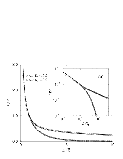
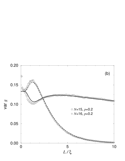
FIG. 6.: The average (a) and the variance (b) of the conductance $g$ for the random flux model (3) at $\varepsilon=0$ for $N=15$ (circle) and $N=16$ (diamond) with disorder strength $p=0.2$. For these parameters, we find that $\xi=280a$ for $N=15$ and $\xi=283a$ for $N=16$. The solid (dashed) lines in (a) are the theoretical result (49) for $\langle g\rangle$ for $N=15$ ($16$); the solid (dashed) lines in (b) are the large odd (even) $N$ analytical results (69) for $\mbox{var}\,g$.

As in the case of the average conductance, for $\mbox{var}\,g$, the even-odd effect can be clearly seen for $L\gtrsim\xi$, where the numerical data coincide with the analytic result in the large $N$ limit, Eq. (69). The slight discrepancy at very small $L$ happens at $M\sim N$ and may be understood as a crossover from quasi one-dimensional to quasi two-dimensional behavior. This type of one- to two-dimensional crossover was reported in a numerical work by Tamura and Ando.[88] The Fokker-Planck approach employed in sections II and III is specifically devised for a quasi one-dimensional geometry and is therefore inapplicable to describe the regime $M\lesssim N$.

In Figs. 7 and 8 we consider the dependence of $\langle g\rangle$ and $\mbox{var}\,g$ on $N$, $p$, and $\varepsilon$. Figure 7(a) shows the average and variance of $g$ for odd $N$ at $\varepsilon=0$ for two choices of $N$ and $p$. We see that the numerical data show fairly good agreement with the analytic large $N$ result (solid lines) for the three cases we examined. For larger disorder strength $p$, the deviations from the analytical result (69) is more prominent, the stronger disorder data being closer to the onset of quasi two-dimensional behavior for small $L$. The agreement between the numerical data for $p=1$ and the theory of Sec. III for $L\gg\xi$ is remarkable, in view of the fact that the theory was derived under the assumption of weak disorder, whereas $p=1$ corresponds to the strongest possible disorder in the random flux model.

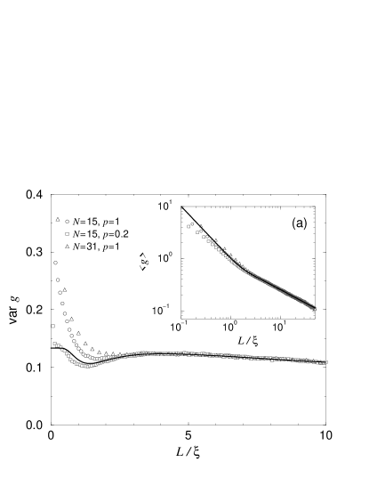
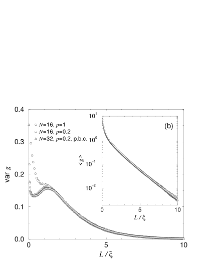
FIG. 7.: The average and the variance of the conductance $g$ for the random flux model (3) at $\varepsilon=0$ for odd $N$ (a) and even $N$ (b). (a) The circles, squares, and triangles are the results for $(N,p)=(15,1.0)$, $(15,0.2)$, and $(31,1.0)$, respectively. The characteristic length $\xi$ is numerically found to be $\xi=23.7a$, $280a$, and $39.8a$, respectively. The solid lines are the large odd $N$ analytical result (69). (b) The circles, squares, and triangles are the results for $(N,p)=(16,1.0)$, $(16,0.2)$, and $(32,0.2)$, respectively. In the last case, periodic boundary conditions (p.b.c.) in the transverse directions are used, whereas for the first two cases open boundary conditions are assumed. The localization lengths $\xi$ are found to be $\xi=27.2a$, $283a$, and $476a$, respectively. The white solid lines are the large even $N$ analytical result for the chiral-unitary class of section III.

Figure 7(b) shows $\langle g\rangle$ and $\mbox{var}\,g$ for the random flux model (3) at $\varepsilon=0$ for an even number $N$ of channels. We show the data for three cases $(N,p)=(16,1)$, (16,0.2), and (32,0.2). In the last example we used periodic boundary conditions in the transverse direction instead of the open boundary conditions of Eq. (3). Since $N$ is even, the periodic boundary conditions do not destroy the chiral symmetry, so that the system remains in the chiral unitary symmetry class. We see that the results of numerical simulations are indistinguishable from the theoretical curves (solid lines) for both $\langle g\rangle$ and ${\rm var}\ g$ except in the quasi two-dimensional regime $M\lesssim N$. We conclude from Fig. 7(a) and 7(b) that the localization properties of the random flux model at $\varepsilon=0$ are governed by the chiral unitary universality class, independent of the disorder strength.

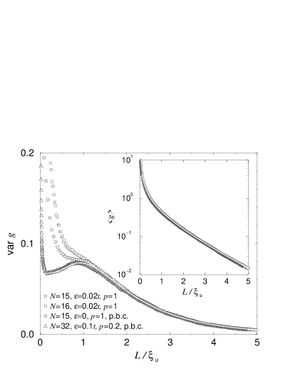
FIG. 8.: Average and variance of $g$ for disorder strength $p=1$ away from the critical energy $\varepsilon=0$. The circles and squares are the data for $N=15$ and $\varepsilon=0.02t$ ($\xi_{\rm u}=47.8a$) and for $N=16$ and $\varepsilon=0.02t$ ($\xi_{\rm u}=50.6a$), respectively. The diamonds and triangles are the data for $N=15$ and $\varepsilon=0$ ($\xi_{\rm u}=45.0a$) and for $N=32$ and $\varepsilon=0.1t$ ($\xi_{\rm u}=1041a$), which are calculated for the periodic boundary condition. For odd $N$, periodic boundary conditions break the chiral symmetry. The white solid lines are the large $N$ analytical result for the unitary class, taken from Refs. [60, 61, 62].

In figure 8 we show some results where the chiral symmetry is broken. In this case, charge transport is no longer governed by the Fokker-Planck equation (II) for the chiral unitary symmetry class, but by the Fokker-Planck equation (1) that is valid for the standard unitary class.[64, 65, 66] In the figure, numerical results are shown for three cases away from the critical energy as well as for one case where the chiral symmetry does not exist because of the periodic boundary condition imposed for odd $N$. With the exception of very short lengths, where the system becomes quasi two-dimensional, all the data for $\langle g\rangle$ and for $\mbox{var}\,g$ agree with the theoretical prediction for the unitary class.[60, 61, 62] The results indicate that the small nonzero energy $\varepsilon=0.02t$ is sufficient to cause a change from the chiral unitary symmetry class at $\varepsilon=0$ to the standard unitary symmetry class. Another interesting feature to note is that the localization length $\xi$ in Fig. 8 is roughly twice as large as that in the chiral case (Fig. 7). (For example, compare the two cases $\varepsilon=0$ and $\varepsilon=0.02t$ for $N=16$ and $p=1$, where we find $\xi=27.2a$ and $\xi_{\rm u}=50.6a$, respectively.) This behavior was observed earlier in Refs. [89, 34, 35]. This result is consistent with the analytic result that $\xi$ differs by a factor of 2 between the chiral ($\xi=N\ell$) and the unitary class ($\xi_{\rm u}=2N\ell$), assuming that the mean free path determined by the short-distance physics is identical in the two classes. (For the numerical results we may expect that the mean free path should not have strong energy dependence on the scale of $|\varepsilon|<0.1t$.)

V Conclusion

In this paper we studied transport properties of a particle on a rectangular lattice in the presence of uncorrelated random fluxes of vanishing mean. This problem is commonly known as the random flux problem. We considered a wire geometry and weak disorder and showed that the symmetries of the random flux problem have dramatic consequences on the statistical distribution of the conductance $g$. If the energy $\varepsilon$ is away from the band center $\varepsilon=0$, the system belongs to the standard unitary symmetry class, while at $\varepsilon=0$, transport is governed by an additional symmetry of the random flux model, the particle-hole or chiral symmetry. We have compared numerical simulations of the average and variance of the conductance $g$ in the random flux model in a thick quantum wire to analytical calculations for the standard unitary and the chiral unitary symmetry classes, and found good agreement for $\varepsilon\neq 0$ and $\varepsilon=0$, respectively.

There are important differences between the conductance distribution in the chiral unitary symmetry class and the standard unitary symmetry class, both in the diffusive and the localized regime. These differences are summarized in Table I. The most striking feature of the chiral unitary symmetry class is the even-odd effect:[34, 63] If the number of channels $N$ in the wire is even, the average conductance $\langle g\rangle$ decays exponentially with length $L$ in the localized regime $L\gg N\ell$, whereas for odd $N$, the decay of $\langle g\rangle$ is algebraic. The sensitivity to the chiral symmetry in transport properties is very strong. For example, removing the chiral symmetry by a change in boundary condition is sufficient to change the universality class to the standard unitary one, even in the thick-wire limit $N\gg 1$.

	unitary	chiral unitary
		even $N$	odd $N$
diffusive
$\langle g\rangle$	${N^{\vphantom{M}}\ell\over L_{\vphantom{M}}}$	${N\ell\over L}$	${N\ell\over L}$
$\mbox{var}\,g$	${1^{\vphantom{M}}\over 15_{\vphantom{M}}}$	${2\over 15}$	${2\over 15}$
localized
$\langle g\rangle$	$\vphantom{M^{M}\over M_{M}}2\left({\pi N\ell\over L}\right)^{3/2}e^{-L/4N\ell}$	$\sqrt{{8N\ell\over\pi L}}e^{-L/2N\ell}$	$\sqrt{{2N\ell\over\pi L}}$
$\mbox{var}\,g$	$\vphantom{M^{M}\over M_{M}}{1\over 2}\left({\pi N\ell\over L}\right)^{3/2}e^{-L/4N\ell}$	$\sqrt{{2N\ell\over\pi L}}e^{-L/2N\ell}$	$\sqrt{{8N\ell\over 9\pi L}}$

TABLE I.: Average and variance of the conductance $g$ of a disordered quantum wire with $N\gg 1$ channels and mean free path $\ell$ in the unitary and chiral unitary symmetry classes, for the diffusive regime $L\ll N\ell$ and for the localized regime $L\gg N\ell$. The results for the unitary ensemble are taken from Refs. [60, 61, 62].

Although our theory is limited to a quasi one-dimensional geometry and cannot account for the crossover from one to two dimensions, it does show the importance of the chiral symmetry to the transport properties of the random flux problem. Taking the prominent role played by symmetry for the random flux model in quasi one-dimension as a guideline, we speculate that a similar picture is appropriate for the two-dimensional random flux problem. Hence, following Gade and Wegner,[48] and Miller and Wang[34] we expect that the localization properties of the two-dimensional random flux problem are controlled by the unitary symmetry class away from the band center $\varepsilon=0$, whereas the band center $\varepsilon=0$ plays the role of a critical energy. The random flux problem would thus share with the Integer Quantum Hall Effect, and with the problem of Dirac fermions in a random vector potential the existence of a single critical energy that lies between energies with localized states. There are however two important differences with the Integer Quantum Hall Effect. First, there is no symmetry that fixes the value of the critical energy in the Integer Quantum Hall Effect, while the chiral symmetry of the random flux model implies that criticality occurs at the band center $\varepsilon=0$. Second, in contrast to the smooth density of states in the Integer Quantum Hall Effect, one expects that the density of states in the random flux problem is singular at $\varepsilon=0$. Such a singularity of the density of states at $\varepsilon=0$ was observed in the single chain random hopping problem, is suggested by the numerical simulations of Refs. [50, 35], and is consistent with Gade’s analysis of the two-dimensional non-linear-$\sigma$ model with chiral symmetry,[48] and with exact results on the problem of Dirac fermions in a random vector potential.[51, 52] (The latter problem shares the same chiral symmetry as the random flux problem although it differs from the random flux problem in that the magnetic fluxes are strongly correlated on all length scales.)

A Derivation of the Fokker-Planck equation

In this paper, we described the transport properties of a quantum wire in the chiral unitary symmetry class in terms of its transfer matrix ${\cal M}$. Our theoretical analysis was focused on a solution of the Fokker-Planck equation (II) that governs the $L$-evolution of the probability distribution $P(x_{1},\ldots,x_{N};L)$ of the eigenvalues $e^{\pm 2x_{j}}$ of ${\cal M}{\cal M}^{\dagger}$. A derivation of this Fokker-Planck equation from a different microscopic model was presented in Ref. [63]. Here we present an alternative derivation of Eq. (II) that is closer in spirit to derivations of the Fokker-Planck equation for the unitary class existing in the literature.[65]

For the statistical distribution of the parameters $x_{j}$, the symmetries of the transfer matrix ${\cal M}(\varepsilon)$ are of fundamental importance. For the random flux model, there are two symmetries (cf. Sec. II):

$${\cal M}(\varepsilon)\,\Sigma_{3}\,{\cal M}^{\dagger}(\varepsilon)=\Sigma_{3},\ \ \mbox{flux conservation},$$ (A1)

$$\Sigma_{1}{\cal M}(\varepsilon)\Sigma_{1}={\cal M}(-\varepsilon),\ \ \mbox{chiral symmetry}.$$ (A2)

Here the transfer matrix ${\cal M}$ is defined in Eq. (4) and $\Sigma_{j}=\sigma_{j}\otimes\openone_{N}$, where $\sigma_{j}$ is the Pauli matrix ($j=1,3$) and $\openone_{N}$ is the $N\times N$ unit matrix.

Because of flux conservation (A1) ${\cal M}(\varepsilon)$ can be parameterized as[66]

$${\cal M} = \pmatrix{{\cal M}_{11}&{\cal M}_{12}\cr{\cal M}_{21}&{\cal M}_{22}\cr}$$ (A3)

$$= \pmatrix{{\cal U}&0\cr 0&{\cal U}^{\prime}\cr}\pmatrix{\cosh X&\sinh X\cr\sinh X&\cosh X\cr}\pmatrix{{\cal V}&0\cr 0&{\cal V}^{\prime}\cr},$$ (A4)

where ${\cal U}$, ${\cal U}^{\prime}$, ${\cal V}$, and ${\cal V}^{\prime}$ are $N\times N$ unitary matrices and $X$ is a diagonal matrix containing the parameters $x_{j}$ on the diagonal. We are interested in the case of zero energy, when the chiral symmetry (A2) results in the further constraints ${\cal U}={\cal U}^{\prime}$ and ${\cal V}={\cal V}^{\prime}$. Notice that in this case, with the parameterization (A4), the parameters $x_{j}$ are uniquely determined by ${\cal M}$. This is an important difference with the unitary symmetry class, where each $x_{j}$ is only defined up to a sign. As a result, in the unitary class, the distribution $P(x_{1},\ldots,x_{N};L)$ has to be symmetric under a transformation $x_{j}\to-x_{j}$ for each $j$ individually, while no such symmetry requirement exists in the chiral unitary class.[90]

FIG. 9.: A thin slice of length $\delta L$ with $a\ll\delta L\ll\ell\ll L$ is added to the disordered region of length $L$.

As the length $L$ of the disordered region is increased (see Fig. 9), the parameters $x_{j}$, $j=1,\ldots,N$ are subjected to a Brownian motion process: As $L$ is increased by an amount $\delta L$, the parameters $x_{j}$ will undergo a (random) shift $x_{j}\to x_{j}+\delta x_{j}$. We first seek the appropriate Langevin equations that describe the statistical distribution of the increments $\delta x_{j}$. Hereto we note that the transfer matrix $\hat{\cal M}\equiv{\cal M}(0;L+\delta L)$ is the product of the individual transfer matrices ${\cal M}\equiv{\cal M}(0;L)$ and ${\cal M}^{\prime}\equiv{\cal M}(0;\delta L)$ for wires of length $L$ and $\delta L$, respectively:

$$\hat{\cal M}={\cal M}{\cal M}^{\prime}.$$ (A5)

We also use that the matrix

$$2{\cal M}_{11}{\cal M}_{12}^{\dagger}={\cal U}\,\sinh(2X)\,{\cal U}^{\dagger}$$ (A6)

is hermitian and has eigenvalues $\sinh 2x_{j}$, $j=1,\ldots,N$. Hence we find that

$$2\hat{\cal M}_{11}\hat{\cal M}_{12}^{\dagger} = {\cal U}\left(\sinh 2X+2\Delta\right){\cal U}^{\dagger},$$ (A7)

$$\Delta = {\cal U}^{{\dagger}}\left(\hat{\cal M}^{\ }_{11}\,\hat{\cal M}^{{\dagger}}_{12}\,-\,{\cal M}^{\ }_{11}\,{\cal M}^{{\dagger}}_{12}\right){\cal U}.$$ (A8)

Making use of the symmetries of ${\cal M}^{\prime}$ and of the parameterization (A4) we can rewrite $\Delta$ as

$$\Delta = \cosh X\,{\cal V}{\cal M}_{12}^{\prime}{\cal M}_{12}^{\prime\dagger}{\cal V}^{\dagger}\,\sinh X$$ (A12)

$$\mbox{}+\sinh X\,{\cal V}{\cal M}_{12}^{\prime}{\cal M}_{12}^{\prime\dagger}{\cal V}^{\dagger}\,\cosh X$$

$$\mbox{}+\cosh X\,{\cal V}{\cal M}_{11}^{\prime}{\cal M}_{12}^{\prime\dagger}{\cal V}^{\dagger}\,\cosh X$$

$$\mbox{}+\sinh X\,{\cal V}{\cal M}_{12}^{\prime}{\cal M}_{11}^{\prime\dagger}{\cal V}^{\dagger}\,\sinh X.$$

We take the length $\delta L$ of the added slice small compared to the mean free path $\ell$. Within the thin slice the disorder is assumed to be uncorrelated beyond a length scale of the order of the lattice spacing $a\ll\delta L$. In this case one has ${\cal M}^{\prime}=1+{\cal O}(\delta L)^{1/2}$, so that the matrix $\Delta$ is of order $(\delta L)^{1/2}$ itself and we can treat it in perturbation theory. As a result, we find that the addition of the slice of width $\delta L$ results in the change

$$\sinh 2\hat{x}_{j}-\sinh 2x_{j} = 2\Delta_{jj}+4\sum_{k\neq j}{\Delta_{jk}\Delta_{kj}\over\sinh 2x_{j}-\sinh 2x_{k}}$$ (A14)

$$\mbox{}+{\cal O}(\delta L^{3/2}),$$

or equivalently

$$\delta x_{j} = {\Delta_{jj}\over\cosh 2x_{j}}-{\Delta_{jj}^{2}\sinh 2x_{j}\over\cosh^{3}2x_{j}}$$ (A17)

$$\mbox{}+2\sum_{k\neq j}{\Delta_{jk}\Delta_{kj}\over(\sinh 2x_{j}-\sinh 2x_{k})\cosh 2x_{j}}$$

$$\mbox{}+{\cal O}(\delta L^{3/2}).$$

It remains to find the first two moments of $\Delta_{jk}$. Hereto we make an ansatz for the distribution of the transfer matrix ${\cal M}^{\prime}$. Because ${\cal M}^{\prime}$ is close to $1$, it is natural to parameterize it in terms of its generator,

$${\cal M}^{\prime}=\exp\,{\cal A}.$$ (A18)

From the symmetry requirements (A1) and (A2) we deduce that ${\cal A}$ has the form

$${\cal A}=iV\otimes\openone_{2}+W\otimes\sigma_{1},$$ (A19)

where $V$ and $W$ are hermitian $N\times N$ matrices. We choose a convenient statistical distribution of ${\cal M}^{\prime}$ by assuming that $V$ and $W$ have independent, Gaussian distributions with zero mean and with variance

$$\langle V_{ij}V_{kl}\rangle=\langle W_{ij}W_{kl}\rangle=\delta_{il}\delta_{jk}{\delta L\over N\ell}.$$ (A20)

Then we find that the first two moments of $\Delta$ are given by

$$\langle\Delta_{jk}\rangle = \delta_{jk}\sinh(2x_{j}){\delta L\over\ell},$$

$$\langle\Delta_{jk}\Delta_{kj}\rangle = \cosh^{2}(x_{j}+x_{k}){\delta L\over N\ell}.$$

Combining this with Eq. (A17), we conclude that under addition of a narrow slice of width $\delta L\ll\ell$, the parameters $x_{j}$ undergo a shift $x_{j}\to x_{j}+\delta x_{j}$ with

$$\langle\delta x_{j}\rangle_{\delta L}={\delta L\over N\ell}\sum_{k\neq j}\coth(x_{j}-x_{k}),$$ (A22)

$$\langle\delta x_{j}\delta x_{k}\rangle_{\delta L}={\delta L\over N\ell}\delta_{jk},$$ (A23)

all higher moments vanishing to first order in $\delta L$. Equation (A) is equivalent to the Fokker-Planck equation (II).

B Solution to the Fokker-Planck equation

In this appendix, we present an exact solution for the Fokker-Planck equation (II), closely following the exact solution of the DMPK equation in the unitary symmetry class by Beenakker and Rejaei.[67] We start by rewriting Eq. (II) as

$$\ell{\partial P\over\partial L} = {1\over 2N}\sum_{j=1}^{N}{\partial\over\partial x_{j}}\left[{\partial P\over\partial x_{j}}+2P\left({\partial\Omega\over\partial x_{j}}\right)\right],$$ (B2)

$$\Omega = -{1\over 2}\sum_{j<k}\ln|\sinh(x_{j}-x_{k})|^{2},$$ (B3)

where the initial condition is

$$P(x_{1},\ldots,x_{N};0)=\prod_{j=1}^{N}\delta(x_{j}).$$ (B4)

The key step towards the exact solution of Eq. (B) is the transformation

$$P(\{x_{j}\};L)=\left[\prod_{j<k}\sinh(x_{j}-x_{k})\right]\Psi(\{x_{j}\};L),$$ (B5)

which changes the Fokker-Planck equation (B) into a Schrödinger equation,

$$-\ell{\partial\Psi\over\partial L} = -{1\over 2N}\sum_{j=1}^{N}{\partial^{2}\Psi\over\partial x^{2}_{j}}+{1\over 2N}\Psi\,\sum_{j=1}^{N}\left[\left({\partial\Omega\over\partial x_{j}}\right)^{2}-{\partial^{2}\Omega\over\partial x^{2}_{j}}\right]$$ (B6)

$$= -{1\over 2N}\sum_{j=1}^{N}{\partial^{2}\Psi\over\partial x^{2}_{j}}+U\Phi.$$ (B7)

Here $U=(N-1)(N-2)/6+(N-1)/2$. Thus, $\Psi(x_{1},\ldots,x_{N};L)$ obeys a Schrödinger equation in imaginary time $L$ that describes $N$ identical free particles on the line, $-\infty<x<\infty$. (For comparison, in the unitary symmetry class, one finds that $\Psi$ obeys a Schrödinger equation for $N$ identical particles moving in the presence of a potential $\propto\sinh^{-2}2x$ which repels the $x$’s away from the origin.[67])

Since the probability distribution $P(x_{1},\ldots,x_{N};L)$ is symmetric under a permutation of the $x_{j}$’s, it follows from Eq. (B5) that $\Psi(x_{1},\ldots,x_{N};L)$ must be antisymmetric, i.e., it must describe the imaginary-time evolution of $N$ identical fermions. At $L=0$, the initial condition (B4) implies that all $x_{j}$ coincide at the origin. Hence, at $L=0$, the transformation (B5) is singular. We avoid this problem by starting with the initial condition[66]

$$P(\{x_{j}\};0|\{y_{k}\}) = {1\over N!}\sum_{\sigma}\prod_{j=1}^{N}\delta(x_{j}-y_{\sigma(j)}),$$ (B8)

$$y_{j}=\epsilon(j-1),$$ (B9)

where all the initial values are different, and send $\epsilon$ to zero at the end of the calculation. The summation is over all permutations $\sigma$ of $1,\ldots,N$.

To solve Eq. (B7), we denote by $G(x;L|y)$ the single-particle Green function of the diffusion equation obeying

$$\ell{\partial G\over\partial L}={1\over 2N}\,{\partial^{2}G\over\partial x^{2}},\qquad G(x;0|y)=\delta(x-y).$$ (B10)

Solution of Eq. (B10) yields

$$G(x;L|y)=\sqrt{N\ell\over 2\pi L}\,e^{-{N\ell\over 2L}(x-y)^{2}}.$$ (B11)

Then the Slater determinant

$$\Psi(\{x_{j}\};L|\{y_{k}\}) = {1\over N!}\,{\rm det}\,\left[G(x_{j};L|y_{k})\right]_{j,k=1,\ldots,N}$$ (B13)

$$\mbox{}\times e^{-UL/\ell}$$

is antisymmetric in $x_{1},\ldots,x_{N}$ and obeys the Schrödinger equation (B7). Using the inverse of the transformation (B5), we obtain that

$$P(\{x_{j}\};L|\{y_{k}\})=$$ (B14)

$$\Psi(\{x_{j}\};L|\{y_{k}\})\prod_{j<k}{\sinh(x_{j}-x_{k})\over\sinh(y_{j}-y_{k})}$$ (B15)

is the solution to the Fokker-Planck equation (B) with the regularized initial condition (B8).

We finally take the limit $\epsilon\to 0$. This limit must be treated with care in view of the denominator of Eq. (B15). With the help of

$${\rm det}\,\left[e^{-{N\ell\over 2L}(x_{j}-y_{k})^{2}}\right]_{j,k=1,\ldots,N}=$$ (B16)

$$e^{-\sum\limits_{j=1}^{N}{N\ell\over 2L}x_{j}^{2}}\left({N\ell\epsilon\over 2L}\right)^{N(N-1)\over 2}\prod_{j<k}(x_{j}-x_{k})+{\cal O}(\epsilon^{2}),$$ (B17)

the singularity $\propto\epsilon^{-N(N-1)/2}$ coming from the denominator in Eq. (B15) is cancelled. We thus recover Eq. (17).

REFERENCES

- [1] Permanent address.
- [2] J. T. Edwards, and D. J. Thouless, J. Phys. C 5, 807 (1972).
- [3] D. C. Licciardello, and D. J. Thouless, J. Phys. C 8, 4157 (1975); 11, 925 (1978).
- [4] F. J. Wegner, Z. Phys. B 25, 327 (1976).
- [5] E. Abrahams, P. W. Anderson, D. C. Licciardello, and T. V. Ramakrishnan, Phys. Rev. Lett. 42, 673 (1979).
- [6] For a review, see P. A. Lee and T. V. Ramakrishnan, Rev. Mod. Phys. 57, 287 (1985).
- [7] F. J. Wegner, Z. Phys. B 35, 207 (1979).
- [8] S. Hikami, A. I. Larkin, and Y. Nagaoka, Prog. Theor. Phys. 63, 707 (1980).
- [9] F. J. Dyson, J. Math. Phys. 3, 140 (1962); 3, 157 (1962); 3, 166 (1962); 3, 1191 (1962); 3, 1199 (1962).
- [10] See, e.g., B. Huckestein, Rev. Mod. Phys. 67, 357 (1995).
- [11] D. E. Khmel’nitskii, Pis’ma Zh. Eksp. Teor. Fiz. 38, 454 (1983) [JETP Lett. 38, 552].
- [12] H. Levine, S. B. Libby, and A. M. M. Pruisken Phys. Rev. Lett. 51, 1915 (1983).
- [13] The Anderson localization in this model was first considered by P. A. Lee and D. S. Fisher, Phys. Rev. Lett. 47, 882 (1981).
- [14] C. Pryor and A. Zee, Phys. Rev. B 46, 3116 (1992).
- [15] B. L. Altshuler and L. B. Ioffe, Phys. Rev. Lett. 69, 2979 (1992).
- [16] D. V. Khveshchenko and S. V. Meshkov, Phys. Rev. B 47, 12 051 (1993).
- [17] G. Gavazzi, J. M. Wheatley, and A. J. Schofield, Phys. Rev. B 47, 15 170 (1993).
- [18] T. Ohtsuki, K. Slevin, and Y. Ono, J. Phys. Soc. Jpn. 62, 3979 (1993).
- [19] T. Sugiyama and N. Nagaosa, Phys. Rev. Lett. 70, 1980 (1993).
- [20] D. K. K. Lee and J. T. Chalker, Phys. Rev. Lett. 72, 1510 (1994); D. K. K. Lee, J. T. Chalker, and D. Y. K. Ko, Phys. Rev. B 50, 5272 (1994).
- [21] A. G. Aronov, A. D. Mirlin, and P. Wölfle, Phys. Rev. B 49, 16 609 (1994).
- [22] Y. B. Kim, A. Furusaki, and D. K. K. Lee, Phys. Rev. B 52, 16 646 (1995).
- [23] J. A. Vergés, Phys. Rev. B 54, 14 822 (1996).
- [24] K. Yakubo and Y. Goto, Phys. Rev. B 54, 13 432 (1996).
- [25] M. Batsch, L. Schweitzer, and B. Kramer, Physica B 249-251, 792 (1998).
- [26] Y. Avishai, Y. Hatsugai, and M. Kohmoto, Phys. Rev. B 47, 9561 (1993).
- [27] V. Kalmeyer, D. Wei, D. P. Arovas, and S. C. Zhang, Phys. Rev. B 48, 11 095 (1993).
- [28] S. C. Zhang and D. P. Arovas, Phys. Rev. Lett. 72, 1886 (1994).
- [29] T. Kawarabayashi and T. Ohtsuki, Phys. Rev. B 51, 10 897 (1995).
- [30] D. Z. Liu, X. C. Xie, S. Das Sarma, and S. C. Zhang Phys. Rev. B 52, 5858 (1995).
- [31] D. N. Sheng and Z. Y. Weng, Phys. Rev. Lett. 75, 2388 (1995).
- [32] K. Yang and R. N. Bhatt, Phys. Rev. B 55, R1922 (1997).
- [33] X. C. Xie, X. R. Wang, and D. Z. Liu, Phys. Rev. Lett. 80, 3563 (1998).
- [34] J. Miller and J. Wang, Phys. Rev. Lett. 76, 1461 (1996).
- [35] A. Furusaki, Phys. Rev. Lett. 82, 604 (1999).
- [36] A. Eilmes, R. A. Römer, and M. Schreiber, Eur. Phys. J. B 1, 29 (1998).
- [37] G. Theodorou and M. H. Cohen, Phys. Rev. B 13, 4597 (1976).
- [38] T. P. Eggarter and R. Riedinger, Phys. Rev. B 18, 569 (1978).
- [39] H. Mathur, Phys. Rev. B 56, 15 794 (1997).
- [40] See F. Wegner, Z. Phys. B 44, 9 (1981).
- [41] F. J. Dyson, Phys. Rev. 92, 1331 (1953).
- [42] B. M. McCoy and T. T. Wu, Phys. Rev. 176, 631 (1968).
- [43] E. R. Smith, J. Phys. C 3, 1419 (1970).
- [44] R. Shankar and G. Murphy, Phys. Rev. B 36, 536 (1987).
- [45] D. S. Fisher. Phys. Rev. B 50, 3799 (1994); 51, 6411 (1995).
- [46] R. H. McKenzie, Phys. Rev. Lett. 77, 4804 (1996).
- [47] L. Balents and M. P. A. Fisher, Phys. Rev. B 56, 12 970 (1997).
- [48] R. Gade, Nucl. Phys. B 398, 499 (1993); R. Gade and F. Wegner, ibid. 360, 213 (1991); F. J. Wegner, Phys. Rev. B 19, 783 (1979).
- [49] S. Hikami, M. Shirai, and F. Wegner, Nucl. Phys. B 408, 413 (1993).
- [50] K. Minakuchi and S. Hikami, Phys. Rev. B 53, 10 898 (1996).
- [51] A. W. W. Ludwig, M. P. A. Fisher, R. Shankar, and G. Grinstein, Phys. Rev. B 50, 7526 (1994).
- [52] A. A. Nersesyan, A. M. Tsvelik, and F. Wenger, Phys. Rev. Lett. 72, 2628 (1994); Nucl. Phys. B 438, 561 (1995).
- [53] C. Mudry, C. Chamon, and X.-G. Wen, Nucl. Phys. B 466, 383 (1996).
- [54] C. de C. Chamon, C. Mudry, and X.-G. Wen, Phys. Rev. Lett. 77, 4194 (1996).
- [55] I. I. Kogan, C. Mudry, and A. M. Tsvelik, Phys. Rev. Lett. 77, 707 (1996).
- [56] H. E. Castillo, C. de C. Chamon, E. Fradkin, P. M. Goldbart, and C. Mudry, Phys. Rev. B 56, 10 668 (1997).
- [57] Y. Hatsugai, X.-G. Wen, and M. Kohmoto, Phys. Rev. B 56, 1061 (1997); Y. Morita and Y. Hatsugai, Phys. Rev. Lett. 79, 3728 (1997), and Phys. Rev. B 58, 6680 (1998).
- [58] J.-S. Caux, N. Taniguchi, and A. M. Tsvelik, Phys. Rev. Lett. 80, 1276 (1998).
- [59] C. Mudry, B. D. Simons, and A. Altland, Phys. Rev. Lett. 80, 4257 (1998).
- [60] M. R. Zirnbauer, Phys. Rev. Lett. 69, 1584 (1992).
- [61] A. D. Mirlin A. Müller-Groeling, and M. R. Zirnbauer, Ann. Phys. (N.Y.) 236, 325 (1994).
- [62] K. Frahm, Phys. Rev. Lett. 74, 4706 (1995).
- [63] P. W. Brouwer, C. Mudry, B. D. Simons, A. Altland, Phys. Rev. Lett. 81, 862 (1998).
- [64] O. N. Dorokhov, Pis’ma Zh. Eksp. Teor. Fiz. 36, 259 (1982) [JETP Letters 36, 318].
- [65] P. A. Mello, P. Pereyra, and N. Kumar, Ann. Phys. (NY) 181, 290 (1988).
- [66] For a reviews, see: A. D. Stone, P. A. Mello, K. A. Muttalib, and J.-L. Pichard in Mesoscopic Phenomena in Solids, edited by B. L. Altshuler, P. A. Lee, and R. A. Webb (North Holland, Amsterdam, 1991); C. W. J. Beenakker, Rev. Mod. Phys. 69, 731 (1997).
- [67] C. W. J. Beenakker and B. Rejaei, Phys. Rev. Lett. 71, 3689 (1993); Phys. Rev. B 49, 7499 (1994).
- [68] This even-odd effect was also observed numerically by W. L. Chan, X. R. Wang, and X. C. Xie, Phys. Rev. B 54, 11213 (1996).
- [69] V. Kalmeyer and S. C. Zhang, Phys. Rev. B 46, 9889 (1992).
- [70] B. I. Halperin, P. A. Lee, and N. Read, Phys. Rev. B 47, 7312 (1993).
- [71] N. Nagaosa and P. A. Lee, Phys. Rev. Lett. 64, 2450 (1990).
- [72] For reviews, see J-P. Bouchaud, and A. Georges, Phys. Rep. 4, 127 (1990); M. B. Isichenko, Rev. Mod. Phys. 64, 961 (1992).
- [73] J. T. Chalker and Z. Jane Wang, Phys. Rev. Lett. 79, 1797 (1997).
- [74] H. J. Sommers, A. Crisanti, H. Sompolinsky, and Y. Stein, Phys. Rev. Lett. 60, 1895 (1988); Y. V. Fyodorov, B. A. Khoruzhenko, H.-J. Sommers, Phys. Lett. A 226, 46 (1997).
- [75] N. Hatano and D. R. Nelson, Phys. Rev. Lett. 77, 570 (1996).
- [76] K. B. Efetov, Phys. Rev. Lett. 79, 491 (1997).
- [77] F. D. M. Haldane, Phys. Lett. 93A, 464 (1983); Phys. Rev. Lett. 50, 1153 (1983).
- [78] For a review, see E. Dagotto and T. M. Rice, Science 271, (1996).
- [79] R. Landauer, Philos. Mag. 21, 863 (1970).
- [80] D. S. Fisher and P. A. Lee, Phys. Rev. B 23, 6851 (1981).
- [81] The mean free path in Eq. (II) differs a factor from the one used in Ref. [63]. The choice made in Eq. (II) ensures that in the diffusive regime the average conductance is given by the Drude formula .
- [82] M. L. Mehta, Random Matrices, (Academic, New York, 1991), 2nd ed., chapter 5.
- [83] K. A. Muttalib, J. Phys. A 28, L159 (1995).
- [84] We use the notation for Jacobi’s theta functions of Gradshteyn and Ryzhik, chapter 8.18, in Table of Integrals Series and Products, fifth edition, Academic Press (1994).
- [85] A. MacKinnon and B. Kramer, Z. Phys. B 53, 1 (1983).
- [86] T. Ando, Phys. Rev. B 40, 5325 (1989) and references therein.
- [87] H. U. Baranger, D. P. DiVincenzo, R. A. Jalabert, and A. D. Stone, Phys. Rev. B 44, 10 637 (1991).
- [88] H. Tamura and T. Ando, Phys. Rev. B 44, 1792 (1991).
- [89] T. Sugiyama, master thesis (unpublished), Univ. of Tokyo (1993).
- [90] An equivalent way to deal with the non-uniqueness of the parameters appearing in the parameterization (A4) for the unitary class is to require that all are positive. In that picture, the are positive for the unitary class, while they can be both positive and negative for the chiral unitary class.