Ground-state dispersion and density of states from path-integral Monte Carlo.
Application to the lattice polaron

Abstract

A formula is derived that relates the ground-state dispersion of a many-body system with the end-to-end distribution of paths with open boundary conditions in imaginary time. The formula does not involve the energy estimator. It allows direct measurement of the ground-state dispersion by quantum Monte Carlo methods without analytical continuation or auxiliary fitting. The formula is applied to the lattice polaron problem. The exact polaron spectrum and density of states are calculated for several models in one, two, and three dimensions. In the adiabatic regime of the Holstein model, the polaron density of states deviates spectacularly from the free-particle shape.

]

I Introduction

Usually, quantum Monte Carlo (QMC) methods are used to study ground-state, thermodynamic, or static properties of quantum-mechanical systems. Some important dynamical characteristics can also be obtained through various forms of fluctuation-dissipation relations. Examples of these are the superfluid fraction of Bose-liquids [1], the Drude weight of conductors [2], the Meissner fraction of superconductors [2], and the effective mass of defects [3, 4] and polarons [5, 6]. Beyond that dynamical calculations are less straightforward. For instance, calculation of the excitation spectrum normally requires measurement of the Green’s function at imaginary times and subsequent analytical continuation to real times.

However, there exists one special type of excitation spectrum that can be measured directly by QMC. This is the ground-state dispersion, i.e., the total energy of the system $E_{\bf P}$ as a function of the total momentum P. In a translationally-invariant system, P is a constant of motion, and the Hamiltonian does not mix subspaces with different P. Then, if a QMC is designed as to operate within a given P-subspace only, it may be able to access the ground state for the given P, thereby providing $E_{\bf P}$. Not for any physical system $E_{\bf P}$ is of interest. For a collection of identical particles, for instance, one has simply $E_{\bf P}={\bf P}^{2}/(2M)$, $M$ being the total mass, which corresponds to free movement of the system as a whole. Positive examples include cases when the system can be divided into a tagged particle and an environment (usually bosons). The best known example of this kind is the polaron, i.e., an electron strongly interacting with phonons. In this case $E_{\bf P}$ is nothing but the polaron spectrum. The polaron spectrum will be the main subject of this paper.

There exist at least two different strategies of how to operate within a restricted P-subspace. The first one is to work in momentum space and to fix the total momentum of the system from outset. An example of this approach is the diagrammatic method of Prokof’ev and Svistunov [7]. In this method QMC is used to sum the entire diagrammatic series for an imaginary-time Green’s function $G({\bf P},\tau)$. Since the total momentum is an external parameter of the series, it is possible to extract $E_{\bf P}$ from the $\tau\rightarrow\infty$ limit behavior of $G$, by fitting it to a single exponential $e^{-E_{\bf P}\tau}$. This method is exact and universal but requires a separate simulation for each P-point.

The second strategy is to work in real space but to use Fourier-type projection operators to project on states with definite P. This amounts to the free boundary conditions in imaginary-time. Usually, the projections are used to calculate the second derivative of the energy with respect to momentum (effective mass) [3, 4]. In Ref. [6] the projection was applied for the first time to the whole polaron spectrum. In this scheme, the ground-state dispersion is measured directly, and all $E_{\bf P}$ are calculated simultaneously. Unfortunately, at non-zero P the weight of the polaron path is no longer positive definite, and one needs to deal with a sign-problem. It turns out, however, that the main idea can be reformulated in a way that does not require a division by the average sign, but only taking its logarithm. While the new formulation does not constitute a complete elimination of the sign-problem, it is more statistically stable and extends the parameter domain accessible in practical simulations. Below we derive the new formula, discuss its properties, and apply to the physically interesting example of the lattice polaron.

II A formula for the ground-state dispersion

Up to our knowledge, the projection relations required for our purposes were first derived by Basile [3] . For completeness a derivation is given below. Let $R$ denote a many-body real-space configuration, and $R+{\bf r}$ a many-body configuration which is a result of the parallel transport of $R$ by a vector ${\bf r}$. (Note that the sum of $R$ and r is only symbolic. The dimensionality of $R$ is equal to the number of degrees of freedom, i.e., very large or infinite, while the dimensionality of r is the dimensionality of space, i.e. 1, 2, or 3.) States $|R\rangle$ form a complete orthogonal basis, ${\bf I}=\int dR\,|R\rangle\langle R|$, and $\langle R|R^{\prime}\rangle=\delta(R-R^{\prime})$. A different basis is formed by the states $|n\rangle$ which are characterized by the definite total momentum ${\bf P}$. One is interested in the projected partition function $Z_{\bf P}$ which includes only states with the given P:

$$Z_{\bf P} \equiv \sum_{n}\langle n|e^{-\beta H}|n\rangle\delta_{{\bf P},{\bf P}_{n}}$$ (1)

$$= \int dR\,dR^{\prime}\langle R^{\prime}|e^{-\beta H}|R\rangle\cdot Q_{\bf P},$$ (2)

$$Q_{\bf P}=\sum_{n}\langle R|n\rangle\langle n|R^{\prime}\rangle\,\delta_{{\bf P},{\bf P}_{n}}=\langle R|{\bf P}\rangle\langle{\bf P}|R^{\prime}\rangle,$$ (3)

where $\beta=(k_{B}T)^{-1}$ is the inverse temperature and $H$ is the full Hamiltonian. The meaning of Eq. (3) is that the two configurations, $R$ and $R^{\prime}$, have to be projected on the given momentum ${\bf P}$. This is achieved as follows (below $\hbar=1$ is set). Any arbitrary configuration $R$ generates a set of states $|{\bf P}_{R}\rangle=V^{-1/2}\int d{\bf r}e^{-i{\bf Pr}}|R+{\bf r}\rangle$, where $V$ is the volume. Inversely, $|R+{\bf r}\rangle=V^{-1/2}\sum_{\bf P}e^{i{\bf Pr}}|{\bf P}_{R}\rangle$. Upon projection, only P-components of both configurations survive. As a result

$$Q_{\bf P} = \frac{1}{V}\int d{\bf r}\langle R+{\bf r}|{\bf P}\rangle\langle{\bf P}|R^{\prime}+{\bf r}\rangle$$ (4)

$$= \frac{1}{V^{2}}\int d{\bf r}\sum_{\bf P^{\prime}P^{\prime\prime}}e^{i({\bf P^{\prime}-P^{\prime\prime}}){\bf r}}\langle{\bf P^{\prime}}_{R}|{\bf P}\rangle\langle{\bf P}|{\bf P^{\prime\prime}}_{R^{\prime}}\rangle$$ (5)

$$= \frac{1}{V}\langle{\bf P}_{R}|{\bf P}_{R^{\prime}}\rangle$$ (6)

$$= \frac{1}{V^{2}}\int d{\bf r}\,d{\bf r^{\prime}}\,\langle R+{\bf r}|R^{\prime}+{\bf r^{\prime}}\rangle\,e^{i{\bf P}({\bf r}-{\bf r^{\prime}})}$$ (7)

$$= \frac{1}{V}\int d(\triangle{\bf r})\langle R+\triangle{\bf r}|R^{\prime}\rangle\,e^{i{\bf P}\triangle{\bf r}}$$ (8)

$$= \frac{1}{V}\int d(\triangle{\bf r})\,e^{i{\bf P}\triangle{\bf r}}\delta((R+\triangle{\bf r})-R^{\prime}),$$ (9)

where $\triangle{\bf r}={\bf r}-{\bf r}^{\prime}$. Substitution in Eq. (2) and integration over $R^{\prime}$ yields

$$Z_{\bf P} = \frac{1}{V}\int\!d(\triangle{\bf r})\,e^{i{\bf P}\triangle{\bf r}}\!\int\!dR\langle R+\triangle{\bf r}|e^{-\beta H}|R\rangle$$ (10)

$$= \frac{1}{V}\int\!d(\triangle{\bf r})\,e^{i{\bf P}\triangle{\bf r}}\!\int\!dR\rho(R,R+\triangle{\bf r};\beta),$$ (11)

where $\rho(R,R^{\prime};\beta)$ is the full many-body density matrix. Next, we assume that for each P the state with the lowest energy $E_{\bf P}$ is non-degenerate, and in the low-temperature limit the projected partition function is dominated by the contribution from this state, $Z_{\bf P}\rightarrow\exp(-\beta E_{\bf P})$. Now take the ratio of $Z_{\bf P}$ and $Z_{{\bf P}=0}$:

$$e^{-\beta(E_{\bf P}-E_{0})} = \lim_{\beta\rightarrow\infty}\frac{Z_{\bf P}}{Z_{{\bf P}=0}}$$ (12)

$$= \lim_{\beta\rightarrow\infty}\frac{\int\!d(\triangle{\bf r})\,e^{i{\bf P}\triangle{\bf r}}\!\int\!dR\rho(R,R+\triangle{\bf r};\beta)}{\int\!d(\triangle{\bf r})\,\int\!dR\rho(R,R+\triangle{\bf r};\beta)},$$ (13)

where $E_{0}$ is the ground-state energy. The rhs is nothing but the average value of $\cos{\bf P}\triangle{\bf r}$ taken over the distribution $\rho$. [We have assumed that $\int dR\rho(R,R+\triangle{\bf r};\beta)$ is an even function of $\triangle{\bf r}$.] A simple formula for $E_{\bf P}$ now follows

$$E_{\bf P}-E_{0}=-\lim_{\beta\rightarrow\infty}\frac{1}{\beta}\ln\langle\cos{\bf P}\triangle{\bf r}\rangle,$$ (14)

which is the main result of this section.

Eq. (14) shows that the ground-state dispersion can be obtained from the end-to-end distribution of many-body paths. It offers a direct way of evaluating the ground-state dispersion by QMC methods in cases when $\rho(R,R^{\prime};\beta)$ is positive-definite. However, the QMC process must be organized in a special way, as apparent from Eq. (12). It must generate only such paths whose end configurations at imaginary time $\tau=\beta$ are exact images of the end configurations at $\tau=0$ except for a parallel transport by an arbitrary vector $\triangle{\bf r}$. It is allowed to change $\triangle{\bf r}$, make simultaneous changes of both end configurations, and to make arbitrary changes of paths at internal times $0<\tau<\beta$, but the end configurations must always be kept identical up to a shift. It is important that this restriction affects neither the ergodicity nor the applicability of the Metropolis algorithm.

Formula (14) involves only one measures quantity, $\langle\cos{\bf P}\triangle{\bf r}\rangle$, instead of two in the previous formulation. Moreover, it does not require division by the measured quantity, but only taking its logarithm. Additionally, Eq. (14) provides the difference between two large numbers, $E_{\bf P}$ and $E_{0}$, and a large cancellation of errors may occur. This makes Eq. (14) much more stable statistically than explicit energy estimators.

On the other hand, at small temperatures, the average cosine becomes exponentially small and it cannot be measured reliably. This reflects the fact that configurations with $E_{\bf P}-E_{0}\gg k_{B}T$ are very rare because of the Boltzmann factor. Thus, the present method is limited to excitation energies of the order of several $k_{B}T$.

III Application to the lattice polaron

We now demonstrate the practical importance of Eq. (14) on the model problem of lattice polaron, which is often considered as a paradigmatic example of a particle strongly interacting with a boson field. We consider a hypercubic lattice with the nearest-neighbor hopping, dispersionless phonons, and the “density-displacement” electron-phonon interaction. The model Hamiltonian reads

$$H=-t\sum_{\langle{\bf nn^{\prime}}\rangle}c^{\dagger}_{\bf n}c_{\bf n^{\prime}}-\sum_{\bf nm}f_{\bf m}({\bf n})c^{\dagger}_{\bf n}c_{\bf n}\xi_{\bf m}+\hbar\omega\sum_{\bf m}b^{\dagger}_{\bf m}b_{\bf m}.$$ (15)

Here $t$ is the hopping amplitude (it will be used as the energy unit), $\omega$ is the phonon (oscillator) frequency, $\xi_{\bf m}$ is the internal coordinate of the mth oscillator, and $f_{\bf m}({\bf n})$ is the force between mth oscillator and the particle at site n ($f$ is a function of distance $|{\bf m-n}|$ only). The model is parametrized by the dimensionless frequency $\bar{\omega}=\hbar\omega/t$ and by the dimensionless coupling constant $\lambda=[\sum_{\bf m}f^{2}_{\bf m}(0)]/(2M\omega^{2}\,D)$, where $M$ is the mass of the oscillator and $D$ is the half-bandwidth of the bare band. (For an isotropic band with nearest-neighbor hopping, $D=zt$, $z$ being the number of neighbors.)

For the polaron problem, a many-body configuration $R$ is specified by the position of the electron r and oscillator displacements $\xi{\bf m}$. Making use of the Feynman’s idea of analytic integration over $\xi{\bf m}$ [8] the problem is reduced to a single-particle system with retarded self-interaction. The latter can be simulated exactly, using the continuous-time representation of polaron paths [9]. The resulting algorithm [6] is very efficient and allow accurate determination of the ground-state energy and effective mass of the polaron for a wide class of models. It this paper, it will be shown that the method also produces accurate polaron spectra, when combined with Eq. (14). There are other reasons why the polaron is an ideal system to try formula (14). First, due to a constant phonon frequency, excited states are, at any P, separated from the restricted ground state by a finite energy gap $\hbar\omega$. Therefore, instead of performing numerically the limit procedure to $\beta=\infty$, one can study the system at finite $\beta$, provided $\exp(\beta\hbar\omega)\gg 1$ and the contribution from excited states is negligible. Second, by increasing the coupling constant $\lambda$ one can always decrease $E_{\bf P}-E_{0}$, i.e., substantially increase $\langle\cos{\bf P}\triangle{\bf r}\rangle$, and stabilise the sumulations. Third, the polaron momentum P is not a parameter of simulations. This implies that statistics can be collected for all momenta simultaneously. In other words, the whole polaron spectrum is measured in a single QMC run. This will enable us to calculate for the first time exact polaron densities of states.

We begin with the simplest Holstein model which has local electron-phonon interaction, $f_{\bf m}({\bf n})=\kappa\delta_{\bf mn}$. In one dimension, the polaron spectrum has been extensively studied by exact diagonalisation [10, 11], strong-coupling perturbation [12], and variational [13] techniques. Our QMC data for the one-dimensional Holstein model are shown in Fig. 1.

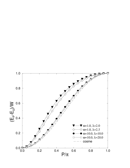
FIG. 1.: Polaron spectrum in the one-dimensional Holstein model, normalized to the bandwidth $W=E_{\pi}-E_{0}$. Triangles: $\bar{\omega}=1.0$, $\lambda=2.0$ [for these parameters the polaron ground-state energy $E_{0}=-4.38(1)$ (in units of $t$), bandwidth $W=0.1243(2)$ (in units of $t$), effective mass $m^{\ast}=10.0(1)$ (in units of $m_{0}=\hbar^{2}/(2ta^{2})$).] Diamonds: $\bar{\omega}=1.0$, $\lambda=2.5$ [$E_{0}=-5.26(1)$, $W=0.0437(3)$, $m^{\ast}=34.5(3)$] . Circles: $\bar{\omega}=10.0$, $\lambda=10.0$ [$E_{0}=-20.35(1)$, $W=0.543(2)$, $m^{\ast}=6.06(2)$] . Squares: $\bar{\omega}=10.0$, $\lambda=20.0$ [$E_{0}=-40.08(1)$, $W=0.0739(2)$, $m^{\ast}=47.6(1)$] .

The most interesting feature of the spectrum is its non-cosine shape in the adiabatic regime $\bar{\omega}\leq 1.0$ (triangles and diamonds). At large momenta, the spectrum is more flat than at small momenta. The nature of this flattening was understood a long time ago [14]. In the weak-coupling limit, the free-particle state hybridizes with the single-phonon state and creates a mixed ground state which is free-particle-like at small P and phonon-like at large P, hence the weak dispersion. With increasing $\lambda$, the free-particle state is replaced with a polaron state with an effective mass $m^{\ast}$, which now hybridizes with the single-phonon state, still leading to a more flat dispersion at large momenta. The flattening effect weakens with growing $\lambda$ and $\bar{\omega}$ because both processes increase the energy separation of the two hybridizing states. In recent years the flattening of the polaron spectrum was observed in numerical studies [10, 12].

Our Quantum Monte Carlo data fully confirm the previous analytical and numerical results, see Fig. 1. We found that the spectrum shape is more sensitive to the phonon frequency than to the coupling constant. At a small frequency $\bar{\omega}=1.0$, the increase of the coupling constant from $\lambda=2.0$ to $\lambda=2.5$ results in a 3.5-times increase of the effective mass, and in a 2.8-times drop of the bandwidth, yet the spectrum shape changes only slightly, cf. triangles and diamonds in Fig. 1. At the same time, a simultaneous 10-times increase of $\lambda$ and $\bar{\omega}$ results in a similar, 4.8 times, increase of effective mass but brings the spectrum shape very close to cosine, cf. triangles and squares in Fig. 1. Again, a doubling of $\lambda$ strongly affects $E_{0}$ and $W$ but not the spectrum shape, cf. circles and squares in Fig. 1.

FIG. 2.: Spectrum of the two-dimensional Holstein model in the adiabatic regime. $\bar{\omega}=1.0$, $\lambda=1.4$. [$E_{0}=-6.12(3)$, $m^{\ast}=8.7(1)$.]

It is instructive to compare the exact QMC results with the Lang-Firsov (LF) approximation [15] which is believed to be the correct description of the polaron in the antiadiabatic regime (high phonon frequency). The LF formula for the spectrum reads

$$E_{P}-E_{0}=2t\,e^{-z\lambda/\bar{\omega}}(1-\cos{P}),$$ (16)

which also implies the relation between the renormalized mass and bandwidth

$$\frac{m^{\ast}}{m_{0}}=\frac{W_{0}}{W}=e^{z\lambda/\bar{\omega}},$$ (17)

where $W_{0}=2zt$ is the bare bandwidth and $m_{0}=\hbar^{2}/(2ta^{2})$ is the bare mass, $a$ being the lattice constant. For $\bar{\omega}=10.0$ and $\lambda=10.0$ QMC results are $W=0.543(2)\,t$ and $m^{\ast}=6.06(2)\,m_{0}$ while LF yields $W_{LF}=0.541\,t$ and $m^{\ast}_{LF}=7.39\,m_{0}$. For $\bar{\omega}=10.0$ and $\lambda=20.0$ one has $W=0.0739(2)\,t$ and $m^{\ast}=47.6(1)\,m_{0}$ from QMC and $W_{LF}=0.0733\,t$ and $m^{\ast}_{LF}=54.6\,m_{0}$ from LF. One can see that LF predicts very accurate values of the polaron bandwidth. This fact was established in the previous studies of the Holstein model [16, 10]. On the other hand, LF slightly overestimates the polaron mass. This is due to small deviations from the cosine shape, still present in the true spectrum at these model parameters. Still, the LF masses are reasonably close to the exact ones, and the agreement improves with the further increase of $\bar{\omega}$ and $\lambda$.

Consider now the two-dimensional Holstein model. The only exact polaron spectra published so far were calculated by Wellein, Fehske, and Loos with the exact diagonalization method [11]. These authors found a flattening of the spectrum in the outer part of the Brillouin zone, even stronger than in the one-dimensional case. We checked that for the model parameters used in [11], formula (14) yields precisely the same values of $E_{\bf P}-E_{0}$ as the exact diagonalization method. A definite advantage of the present method is that it allows simultaneous calculations at any desired number of P-points, while exact diagonalization studies are limited to a small number of P-points due to the finite size of the clusters. On the other hand, the QMC method is limited to the condition $W\ll\hbar\omega$, which prevents us from studying the weak-coupling regime and such an interesting phenomenon as the limit point of the polaron spectrum [14]. (The latter is possible with the diagrammatic QMC [7].) Figure 2 shows our QMC data for a new set of parameters in the adiabatic regime, $\bar{\omega}=1.0$, $\lambda=1.4$, where 30 P-points have been used to represent the spectrum. One can see that the dispersion is indeed weak for $|{\bf P}|>\pi/2$, i.e. in the larger part of the Brillouin zone. Note, that at these parameters the polaron bandwidth is reduced by $8\,t/0.12\,t=67$ times, and the mass enhancement is 8.7, so we are already in the small polaron regime. Yet, the spectrum shape is profoundly non-cosine. With increasing $\lambda$, it will be approaching the cosine shape, but this is expected to happen only at such large $\lambda$ where the polaron is very heavy and is easily localized.

FIG. 3.: Density of states of the two-dimensional Holstein model in the adiabatic regime. $\bar{\omega}=1.0$, $\lambda=1.4$. [$E_{0}=-6.12(3)$, $m^{\ast}=8.7(1)$.]

In two dimensions, the volume of the outer part of the Brillouin zone is larger than that of the inner one. Therefore the linear representation of the spectrum, like in Fig. 2, does not fully convey the changes in the band structure, caused by the flattening of the spectrum. The proper physical quantity which takes into account all the states of the Brillouin zone is the density of states (DOS). The QMC method, coupled with formula (14), provides the unique opportunity to calculate polaron DOS exactly, since it allows a simultaneous measurement of the whole spectrum. In this work, the two-dimensional Brillouin zone was divided in $200^{2}$ points at which the spectrum was measured. In the end, the total of $40\,000$ polaron energies were distributed over 50 energy intervals between 0 and $W$. The resulting DOS for $\bar{\omega}=1.0$, $\lambda=1.4$ (the same parameters as in Fig. 2) is shown in Fig. 3. One can see that the effect of the spectrum flattening is indeed quite dramatic. The upper half-band is jammed into a narrow, $0.015\,t$-width, energy interval, thereby increasing DOS at the top of the band to $\approx 50$ times the DOS at the bottom of the band. The van Hove singularity is shifted from the middle to the top of the band. The lower half of the band contains only $13\%$ of all states. Overall, DOS looks qualitatively different from the free-particle one.

FIG. 4.: Spectrum of the two-dimensional Holstein model in the anti-adiabatic regime. $\bar{\omega}=8.0$, $\lambda=8.0$. [$E_{0}=-32.16(1)$, $m^{\ast}=38.4(1)$.]

FIG. 5.: Density of states of the two-dimensional Holstein model in the anti-adiabatic regime. $\bar{\omega}=8.0$, $\lambda=8.0$. [$E_{0}=-32.16(1)$, $m^{\ast}=38.4(1)$.] Small fluctuations of DOS are artifacts of a finite-mesh integration over the Brillouin zone and not statistical errors.

As in the one-dimensional case, the band structure approaches the free-particle-like as the phonon frequency increases. As an example, we considered a frequency equal to the bare bandwidth, $\bar{\omega}=8.0$, and $\lambda=8.0$. (This value of the coupling constant was chosen to have the polaron bandwidth, $W$, close to the previously considered adiabatic case.) The polaron spectrum and DOS are shown in Figs. 4 and 5, respectively. Deviations from the free-particle behavior are still visible, but they are small and not qualitative. DOS at the top of the band is just $\approx 1.5$ times larger than at the bottom, and the singularity appears close to the middle of the band. The “normalization” of the spectrum at large $\bar{\omega}$ is quite understandable. With increasing phonon frequency, the retardation effects become less important, the lattice deformation more readily follows the particle movement, and the whole complex behaves more like a free particle with a renormalized hopping integral. The Lang-Firsov formula (17) predicts $W_{LF}=0.1465\,t$ and $m^{\ast}_{LF}=54.6\,m_{0}$ which is to be compared with the QMC results $W=0.1510(3)\,t$ and $m^{\ast}=38.4(1)\,m_{0}$. Again, the LF approximation yields the correct bandwidth but overestimates the effective mass by some 40%.

FIG. 6.: Density of states of the three-dimensional Holstein model in the adiabatic regime. $\bar{\omega}=1.0$, $\lambda=1.2$. [$E_{0}=-7.75(4)$, $m^{\ast}=6.2(2)$.]

FIG. 7.: Density of states of the three-dimensional Holstein model in the anti-adiabatic regime. $\bar{\omega}=12.0$, $\lambda=10.0$. [$E_{0}=-60.12(2)$, $m^{\ast}=112(1)$.] Small fluctuations of DOS are artifacts of a finite-mesh integration over the Brillouin zone and not statistical errors.

The most spectacular transformation of DOS occurs in the three-dimensional Holstein model. In three dimensions, the volume of the outer part of the Brillouin zone is much larger than that of the inner part, and it should completely dominate the total DOS. We do not show the polaron spectrum which is not very informative. Density of states was calculated by measuring the polaron spectrum at $60^{3}$ points of the full Brillouin zone, and then distributing them among 50 energy intervals between 0 and $W$. DOS in the adiabatic regime, $\bar{\omega}=1.0$ and $\lambda=1.2$, is shown in Fig. 6. The states of the flat part of the spectrum form a massive peak at the top of the band. The width of the peak is about $10\%$ of the total bandwidth. DOS at the bottom of the band is negligible, the capacity of the lower half-band is less than $1\%$ of the total number of states. The two van Hove singularities are not visible, at least on the chosen level of energy resolution, they are absorbed into the peak. Overall, DOS is completely different from the free-particle one. Should the three-dimensional Holstein model with such parameters exist in nature, an extreme care would be necessary in interpreting experimental data. In any real material, the lowest states would likely be localized, and any response to an external perturbation would be dominated by the peak. Then, for instance, fitting to a free-particle-like form of DOS would lead to wrong estimates of the coupling constant and other errors.

As before, the band structure returns to the free-particle shape in the anti-adiabatic regime. We considered the case of the phonon frequency being equal to the bare bandwidth, $\bar{\omega}=12.0$, and coupling constant $\lambda=10.0$, when the polaron bandwidth is close to the just considered adiabatic case, see Fig. 7. Although still distorted, the DOS shape is close to the free-particle one, with the square-root behavior at the top and the bottom of the band, and with two van Hove singularities fully developed at the “right” places. The polaron bandwidth is $W=0.0827(2)\,t$, which is in good agreement with the Lang-Firsov value $W_{LF}=0.0809\,t$, while the polaron mass $m^{\ast}=112(1)\,m_{0}$ is 24% lighter than the LF mass $m^{\ast}_{LF}=148\,m_{0}$.

FIG. 8.: Density of states of the two-dimensional anisotropic Holstein model. $\bar{\omega}=1.0$, $\lambda=1.4$, $t_{y}/t_{x}=0.2$. [$E_{0}=-3.987(3)$, $m^{\ast}_{x}=3.44(1)\,m_{0x}$, $m^{\ast}_{y}=17.54(3)\,m_{0x}$.]

The polaron QMC algorithm of Ref. [6] is not limited to the Holstein model. In fact, it allows studies of arbitrary forms of the electron-phonon interactions (of the density-displacement type), and arbitrary forms of the particle kinetic energy. Combined with Eq. (14), it provides an efficient and exact way of calculating the band structure of a whole class of polaron models. As possibilities are numerous, we have chosen to illustrate the point on two particular examples.

The first example is the anisotropic two-dimensional Holstein model with $\bar{\omega}=1.0$, $\lambda=1.4$ (these parameters are the same as in Figs. 2 and 3), and the bare anisotropy ratio $t_{y}/t_{x}=0.2$. For a free particle with such an anisotropy, the saddle points at $(\pm\pi,0)$ and $(0,\pm\pi)$ have different energies, which results in two singularities in DOS, positioned symmetrically with respect to the center and edges of the band. Polaron DOS, calculated by QMC, is shown in Fig. 8. The flattening effect creates a strong peak at the top of the band which absorbs the higher-energy singularity [at $(\pm\pi,0)$]. At the same time, the second singularity is still clearly visible. Now it appears in the vicinity of the middle of the band.

FIG. 9.: Density of states of the two-dimensional model with long-range electron-phonon interaction. $\bar{\omega}=1.0$, $\lambda=2.75$. [$E_{0}=-11.83(1)$, $m^{\ast}=20.1(1)$.] Small fluctuations of DOS are artifacts of a finite-mesh integration over the Brillouin zone and not statistical errors.

The second example is the two-dimensional polaron model with long-range electron-phonon interaction [combine with the Hamiltonian (15)]:

$$f_{\bf m}({\bf n})=\frac{\kappa}{(|{\bf m}-{\bf n}|^{2}+1)^{3/2}},$$ (18)

where the distance $|{\bf m}-{\bf n}|$ is measured in lattice constants. For this form of the force, $\lambda=1.742\kappa^{2}/(2M\omega^{2}D)$. The model describes a two-dimensional particle interacting with a parallel plane of ions vibrating perpendicular to the plane. It was proposed in Ref.[18], where it was used to model the interaction of holes doped in copper-oxygen planes, with apical oxygens in the layered cuprates. It was found that this long-range (Fröhlich) polaron is much lighter than the short-range Holstein polaron. Here we present the density of states for $\bar{\omega}=1.0$ and $\lambda=2.75$, see Fig. 9. DOS shape is close to the free-particle one, with a single, well-developed singularity in the middle of the band. Note, that we are in the adiabatic regime, at the same frequency $\bar{\omega}=1.0$ where the two-dimensional Holstein polaron has a very distorted DOS, cf. Fig. 3. The comparison of Figs. 9 and 5 shows that a long-range electron-phonon interaction plays the same role as increasing phonon frequency, as far as the flattening effect is concerned.

IV Discussion and conclusions

The main message of this paper is that a path-integral imaginary-time Quantum Monte Carlo is quite capable of direct measuring of real-time spectra. By relaxing the boundary conditions in imaginary time, one allows many-body paths to have arbitrary real-space shift $\triangle{\bf r}$. Then the Fourier transform projects out configurations with a certain total momentum P. The result, expressed by the formula (14), is the ground-state energy as a function of the total momentum. The physical system, where such a ground-state dispersion is of interest, should be carefully chosen.

The role of temperature in this process is two-fold. On one hand, temperature should be made as low as possible to exclude the contribution from the excited states with the same P. On the other hand, only states with $E_{\bf P}-E_{0}\sim k_{B}T$ are excited in the system. This means that the corresponding configurations will be generated by the QMC process in amounts sufficient for a good statistics. For higher-energy states, configurations will be exponentially rare. This is the reason for the average cosine in Eq. (14) to become exponentially small in the low-temperature limit. In this case, the measurement process will be statistically unstable. Thus, the temperature should be of the order of the energy interval one is interested in. The two conditions on the temperature can be reconciled if the energy scale of the ground-state dispersion is much smaller than the energy gap between the ground state and the excited states within the same P-sector. This is realized in the polaron system where one has $W\ll\hbar\omega$ for a wide range of parameters. If this condition is not satisfied, Eq. (14) will be measuring the difference of projected free energies rather than that of ground-state energies.

Eq. (14) shows that in a many-body system there exists a general and simple relation between the ground-state dispersion and the end-to-end distribution of imaginary-time paths. It does not involve the energy estimator, although the latter is required for the separate calculation of $E_{0}$ and $E_{\bf P}$. This might be useful in cases when the evaluation of the energy estimator is computationally costly. There are other computational advantages. First, Eq. (14) involves only the logarithm of one measured quantity, the average cosine. Second, Eq. (14) calculates the difference of two energies both of which may be large. In the polaron problem, typical energies are of the order of a few $t$ but the bandwidth is $W\sim 0.1\,t$. Both $E_{0}$ and $E_{\bf P}$ can be calculated with typical accuracy $0.3-0.5\,\%$. This may result in a sizable error in their difference if the two energies are calculated separately and then subtracted. Eq. (14) produces much more stable energy differences because of the large cancellation of errors between $E_{\bf P}$ and $E_{0}$. In all the spectra presented in this paper, Figs. 1, 2, 4, the statistical errors are smaller that symbols representing the data. Finally, the whole dispersion (as well as $E_{0}$, and derivatives at any P-point) can be calculated during a single QMC run. This property of Eq. (14) also allows fast computation of the density of states.

To demonstrate the practical usefulness of Eq. (14), we have combined it with an exact continuous-time algorithm for the lattice polaron [6], and calculated first detailed polaron spectra and densities of states in two and three dimensions. Although our method of calculating the spectrum is limited to the condition $W\ll\hbar\omega$, i.e., to the intermediate and strong coupling, this is the most physically interesting regime. Together with the weak- and strong-coupling perturbation expansions, the exact diagonalization, density-matrix renormalization group [19], variational, and diagrammatic QMC techniques, the present method covers the whole parameter range of the polaron problems. One can say, that the problem of calculating the exact polaron spectrum has found its solution.

Apart from being a test for Eq. (14), the lattice polaron still has a considerable interest on its own. We have seen in this paper that the polaron spectrum in the adiabatic limit of the Holstein model is generically non-cosine, as was predicted theoretically and recently observed numerically. The flattening has been found to continue well into the strong-coupling regime, where the polaron mass is a few dozens and approaches a hundred. The same conclusion was reached previously in [11]. For physical applications the most interesting regime is when polarons are not very heavy and can be mobile. We conclude that the non-cosine spectrum is typical for the Holstein model in the physically relevant parameter region, i.e., small phonon frequencies and intermediate couplings.

A surprise finding has been the great extent at which the flattening changes the band structure in high dimensions. Density of states is completely changed, van Hove singularities are shifted, low-lying states are almost irrelevant, relations between the effective mass and the bandwidth is broken. We have seen that the combination of dimensionality, phonon frequency, coupling strength, and anisotropy may produce densities of states of various shapes. In such a situation, one should be careful about the interpretation of any experimental data, like the estimation of $\lambda$ or polaron mass from the bandwidth or from the location of singularities. The use of a “naive” model band structure would lead to wrong conclusions.

We have also found that in all dimensions the polaron band structure becomes free-particle-like with increasing phonon frequency. In particular, the spectrum approaches the cosine shape and the effective mass approaches the inverse of the bandwidth. Moreover, numerical values of $W$ are well described by the Lang-Firsov approximation. Thus, our QMC data support the LF approximation as the right description of the polaron in the antiadiabatic regime. At the same time, we have found that LF could still overestimate the polaron mass by a few dozen percent in cases where the bandwidth is predicted correctly.

Finally, we considered a long-range electron-phonon interaction and found a free-particle-like band structure even in the adiabatic regime. In Ref. [18] it was found that in the adiabatic regime polaron masses are well described by the LF approximation. Two conclusions follow from these facts. First, all the unusual properties of the Holstein model caused by the flattening, may be specific to the local electron-phonon interaction and may not be generic polaron properties. Second, the long-range electron-phonon interaction on a lattice seems to have the same effect on the band structure as the increasing phonon frequency. Although it is clear intuitively that a long-range interaction leads to higher mobility of the lattice deformation, details of this mechanism are yet to be fully understood.

The author is grateful to A. S. Alexandrov, D. M. Ceperley, V. Elser, W. M. C. Foulkes, and V. V. Kabanov for useful discussions and communications. This work was supported by EPSRC under grant GR/L40113.

REFERENCES

- [1] E. L. Pollock and D. M. Ceperley, Phys. Rev. B 36, 8343 (1987).
- [2] D. J. Scalapino, S. R. White, and S. C. Zhang, Phys. Rev. B 47, 7995 (1993).
- [3] A. G. Basile, PhD thesis, (Cornell University, 1992).
- [4] M. Boninsegni and D. M. Ceperley, Phys. Rev. Lett. 74, 2288 (1995).
- [5] C. Alexandrou and R. Rosenfelder, Phys. Rep. 215, 1 (1992).
- [6] P. E. Kornilovitch, Phys. Rev. Lett. 81, 5382 (1998).
- [7] N. V. Prokof’ev and B. V. Svistunov, Phys. Rev. Lett. 81, 2514 (1998).
- [8] R. P. Feynman, Phys. Rev. 97, 660 (1955); Statistical Mechanics (Benjamin, Reading, 1972).
- [9] B. B. Beard and U.-J. Wiese, Phys. Rev. Lett. 77, 5130 (1996).
- [10] G. Wellein, H. Röder, and H. Fehske, Phys. Rev. B 53, 9666 (1996).
- [11] G. Wellein, and H. Fehske, Phys. Rev. B 56, 4513 (1997). H. Fehske, J. Loos, and G. Wellein, Z. Phys. B 104, 619 (1997).
- [12] W. Stephan, Phys. Rev. B 54, 8981 (1996).
- [13] A. H. Romero, D. W. Brown, and K. Lindenberg, J. Chem. Phys. 109, 6540 (1998); cond-mat/9809025.
- [14] Y. B. Levinson and É. I. Rashba, Rep. Prog. Phys. 36, 1499 (1973).
- [15] I. G. Lang and Yu. A. Firsov, Zh. Eksp. Teor. Fiz. 43, 1843 (1962) [ Sov. Phys. JETP 16, 1301 (1963)].
- [16] A. S. Alexandrov, V. V. Kabanov, and D. K. Ray, Phys. Rev. B 49, 9915 (1994).
- [17] The algorithm of Ref. [6] is very fast in the small-polaron regime. It is interesting that in calculation of DOS, most of the CPU time is spent on the “dull” evaluation of the cosine in Eq. (14), about times at each P-point.
- [18] A. S. Alexandrov and P. E. Kornilovitch, Phys. Rev. Lett. 82, 807 (1999).
- [19] E. Jeckelmann and S. R. White, Phys. Rev. B 57, 6376 (1998).