Cohesion and conductance of disordered metallic point contacts

Abstract

The cohesion and conductance of a point contact in a two-dimensional metallic nanowire are investigated in an independent-electron model with hard-wall boundary conditions. All properties of the nanowire are related to the Green’s function of the electronic scattering problem, which is solved exactly via a modified recursive Green’s function algorithm. Our results confirm the validity of a previous approach based on the WKB approximation for a long constriction, but find an enhancement of cohesion for shorter constrictions. Surprisingly, the cohesion persists even after the last conductance channel has been closed. For disordered nanowires, a statistical analysis yields well-defined peaks in the conductance histograms even when individual conductance traces do not show well-defined plateaus. The shifts of the peaks below integer multiples of $2e^{2}/h$, as well as the peak heights and widths, are found to be in excellent agreement with predictions based on random matrix theory, and are similar to those observed experimentally. Thus abrupt changes in the wire geometry are not necessary for reproducing the observed conductance histograms. The effect of disorder on cohesion is found to be quite strong and very sensitive to the particular configuration of impurities at the center of the constriction.

]

I Introduction

In a pioneering experiment published in 1996, Rubio, Agraït and Vieira [1] simultaneously measured the force and conductance during deformation and rupture of gold nanocontacts. They observed nano-Newton force oscillations correlated with conductance steps of order $2e^{2}/h$. Similar results were obtained independently by Stalder and Dürig.[2] An explanation of these force fluctuations, based on the response of the conduction electrons to the mechanical deformation of the contact, was proposed by Stafford et al. [3] In this paper, we give an exact numerical solution to the model of Ref. [3], allowing the treatment of any shape of the constriction and the inclusion of disorder.

Conductance quantization has been widely studied in the past decade, both experimentally [4, 5, 6, 7, 8, 9, 10, 11] and theoretically. [8, 12, 13, 14, 15, 16, 17, 18, 19, 20, 21, 22, 23] On the experimental side, it was first measured in a two-dimensional electron gas split-gate and was understood to be a consequence of the quantization of the transverse motion.[4, 5] Each transverse energy subband defines a conduction channel that contributes $2e^{2}/h$ to the conductance. More recently, conductance quantization in units of $2e^{2}/h$ has been observed in three-dimensional metallic quantum wires using various experimental techniques. [6, 7, 8, 9, 10, 11] In this case, the quantization is not so clear-cut, and measurements are in general less reproducible. Therefore, a statistical analysis of a large set of experimental data is usually made. The resulting conductance histograms show well-defined peaks with centers shifted below integer multiples of $2e^{2}/h$. The shifts can be corrected by subtracting a series resistance of a few hundred Ohms. This resistance was originally attributed to the bulk contacts, which are not part of the nanocontact and should thus be subtracted. [7, 9, 10, 11] It has recently been argued, based on theoretical work, [21] that this resistance could also be caused by disorder in the nanowire, in agreement with previous studies of quantum point contacts.[17, 20]

On the theoretical side, the problem of conductance quantization has been investigated using a variety of techniques, both in two and three dimensions. [8, 12, 13, 14, 15, 16, 17, 18, 19, 20, 21, 22, 23] It is found that conductance plateaus are well defined only in constrictions that are smooth on the scale of the Fermi wavelength. [12, 15, 19] Furthermore, the plateaus can also be affected by thermal fluctuations or disorder. Thermal effects, which smoothen out the conductance steps,[14] are important in the case of a two-dimensional electron gas, [4, 5] where the spacing between subbands is of the order of $1K$, but negligible in the case of metallic point contacts, [1, 2, 6, 7, 8, 9, 10, 11] where the spacing between subbands is of the order of $10^{4}K$. The effect of disorder on conductance quantization has been studied both analytically[17, 20, 23] and numerically.[8, 21, 22] Disorder was found to reduce the conductance compared to the ballistic case, leading to shifts of the peaks in the conductance histograms similar to those observed experimentally. We note that most of the theoretical conductance curves were obtained by changing the Fermi energy, in contrast to the experimental situation for a metallic nanowire, where the Fermi energy is an invariant property of the material and the shape of the contact is modified.

The structural transformations of metallic nanocontacts were first studied by Landman and coworkers,[24] and later by others,[8, 18] using molecular dynamics. These simulations suggest that the elongation of a connective neck proceeds through a sequence of abrupt structural transformations, involving a succession of elastic and yielding stages. Within this approach, the conductance is expected to change abruptly due to atomic rearrangements,[8, 18] and the force is expected to follow a sawtooth behavior.[8, 24] The molecular dynamics simulations give rise to the following interpretation[1, 25, 26] of experiments: During elastic stages, the conductance is essentially constant at a quantized value and the magnitude of the force increases with a constant slope, while the yielding stages consist of abrupt relaxations of the atomic structure, giving rise to a sudden change of conductance and force. It was asserted that both the elastic and transport properties of narrow metallic constrictions can be understood on the basis of atomic rearrangements, calculated in the framework of classical lattice dynamics.

It thus came as a surprise when it was discovered[3] that a simple free electron model, which neglects the discrete atomic structure of the constriction, is able to reproduce both the oscillations in the tensile force and the conductance plateaus of Ref. [1]. In this model, each conductance channel is viewed as a long chemical bond which is stretched and broken, giving rise to the observed force oscillations. Similar results were obtained by van Ruitenbeek et al.[27] using a free-electron model and by Yannouleas and Landman,[28] using a slightly more realistic jellium model. However, these studies dealt with closed systems, while the experimental nanowire is a contact between two macroscopic pieces of metal, and is thus an open system. Since mesoscopic effects can be very different in the canonical and grand canonical ensembles, this is an important distinction.

In this paper, we give an exact numerical solution of the free-electron model proposed in Ref. [3]. Our formalism allows us to extend the analytical results of Ref. [3] by treating both non-adiabatic constrictions and disordered wires. We find that the cohesion of short (non-adiabatic) constrictions is increased compared to that of long constrictions. For disordered systems, we obtain conductance histograms which look very similar to those observed experimentally. Our results also suggest that the cohesion of nanowires is quite sensitive to disorder.

The rest of this paper is organized as follows: In section II, we describe our model in which conductance and cohesion are interconnected through the scattering matrix. Section III presents the numerical method, while the results are discussed in section IV. A short summary is given in section V.

II Model and basic quantities

This section introduces our free-electron model. Its simplicity allows to treat both the conductance and the metallic cohesion in a unified way.

A Assumptions

Our model is based on several simplifying assumptions. (i) Free electrons: Gold is known to be rather well described by the model of free electrons where the atomic potentials are neglected.[29] This indicates that the detailed configuration of atoms has little effect on both electronic and cohesive properties. By adopting the free electron model, we eliminate the kinetics of atomic rearrangements, which seem to play a role in actual experiments, at least for thick constrictions.[30] (ii) Independent electrons: We neglect electron-electron interactions. Recent calculations, one based on an extended Thomas-Fermi scheme,[31] the other on the Hartree approximation, [32] suggest that interactions have little effect on the quantities considered here. However, more careful studies will be needed to substantiate this conclusion, as interaction effects are particularly subtle in one-dimensional systems and thin wires. (iii) Smooth constriction: According to molecular dynamics simulations [8, 18, 24, 26] and experiments, [33, 34] the shape of elongated gold nanowires is quite regular. Therefore we model the contact as a smooth constriction, which changes continuously upon deformation. (iv) Constant volume: The volume of the constricted part is assumed to be conserved during the deformation, in agreement with molecular dynamics simulations.[24] Recent experiments[35] indicate that this assumption is not always valid, for instance in the case of mono-atomic chains. (v) Hard-wall boundary conditions: Electrons are confined to a wire due to a smooth attractive ionic potential. We approximate the potential in terms of hard-wall boundary conditions, keeping in mind that the radius of the boundary will be larger than the effective radius defined by the electronic density. [27] (vi) Zero temperature: The thermal population of electronic subbands above the Fermi energy is negligible for nanowires. Therefore we consider the zero-temperature limit, where inelastic scattering processes, e.g. due to phonons or electron-electron collisions, are absent.

B Model

The physics of the problem is similar for two- and three-dimensional wires except that, for a two-dimensional system, (i) the transverse energy levels are nondegenerate, and therefore the steps in the conductance curves are all of height $2e^{2}/h$, and (ii) the surface energy is reduced as compared to that of a three-dimensional wire; this changes the overall slope of the force curves. We restrict ourselves to two dimensions, where the computational effort is much lower.

Our model wire is described by the eigenvalue equation

$$\left[-\frac{\hbar^{2}}{2m}\left(\partial_{x}^{2}+\partial_{z}^{2}\right)+V_{dis}(x,z)\right]\psi(x,z)=E\psi(x,z),$$ (1)

where $x$ and $z$ are the transverse and longitudinal coordinates, respectively, and $V_{dis}(x,z)$ is a potential due to disorder. We use the boundary condition $\psi=0$ for $x^{2}=r^{2}(z)$, where $r(z)$ defines the geometry (see Fig. 1). In the initial configuration, there is no constriction ($r(z)=R$) and the disorder is restricted to a finite part of the wire (namely to $|z|<(L_{0}/2+L_{dis})$, where $L_{0}$ is the initial length of the deformable part). After elongation by $\Delta L=L-L_{0}$, the shape of the deformable part is chosen to be, for $|z|<L/2$,

$$r(z)=R_{min}+(R-R_{min})\left(3u^{2}-3u^{4}+u^{6}\right),$$ (2)

where $u=\left|\frac{2z}{L}\right|$ and $2R_{min}$ is the width of the narrowest part of the constriction, related to $L$ by the condition of constant volume. The specific choice of the function $r(z)$ is not crucial,[3] as has been checked by using other shapes.

FIG. 1.: Schematic diagram of a constriction in a 2D quantum wire. Electrons are confined along the $z$ axis by a hard-wall potential at $x=\pm r(z)$. Localized impurities of potential $V(x-x_{j},z-z_{j})$ are distributed randomly in the constriction and within a part of length $L_{dis}$ on each side of it.

The potential $V_{dis}(x,z)=\sum_{j}V(x-x_{j},z-z_{j})$ describes randomly distributed impurities, with a given density $n_{i}$. It can represent structural defects or real impurities. Similar effects are expected to arise due to surface roughness.[8] During deformation, the impurities are moved in such a way that their local concentration remains constant. Since we are dealing with an open system, we use the grand-canonical ensemble and take the chemical potential to be the Fermi energy of the macroscopic wires connected to the nanocontact. Throughout this paper, we consider the case of gold, with a Fermi energy $\varepsilon_{F}=5.5\,eV$.

C $S$ matrix

The formalism developed by Stafford et al. [3] allows one to treat both transport and mechanical properties of open mesoscopic systems on an equal footing, in terms of the electronic scattering matrix $S$. This formalism is general and can be applied to any non-interacting open system connected to an arbitrary number of leads.

The conductance for the present two lead system is calculated using the Landauer formula[36]

$$G=\frac{2e^{2}}{h}\text{Tr }(t^{\dagger}t),$$ (3)

where $t$ is the transmission matrix at the Fermi energy (directly related to the $S$ matrix).

The force is obtained from the variation of the appropriate free energy, the grand canonical potential $\Omega(\epsilon_{F},L)$, with respect to the length $L$ of the deformed region. For a non-interacting system of electrons, one has

$$\Omega(\epsilon_{F},L)=\int^{\epsilon_{F}}\!dE\left(E-\epsilon_{F}\right)D(E),$$ (4)

where the density of states $D(E)$ is related to the $S$ matrix by [37, 38]

$$D(E)=\frac{1}{2\pi i}\text{Tr }\left\{S^{\dagger}(E)\frac{\partial S}{\partial E}-S(E)\frac{\partial S^{\dagger}}{\partial E}\right\}.$$ (5)

The $S$ matrix provides a fundamental link between conductance and cohesion, and it is amenable to analytical calculations.[3] $S$ is directly related to the retarded electronic Green’s function,[37, 38] which may be calculated numerically, as explained in the next section. A closely related formulation of the free energy in terms of the $S$ matrix was given by Akkermans et al.[39]

III Extended recursive Green’s function method

In this section, we describe our numerical procedure. It consists of computing recursively the Green’s function, from which both the transmission coefficients and the density of states are obtained.

A Green’s function for a wire of constant width

In order to illustrate our method, we first consider an infinite, two-dimensional wire of constant width $2R$. In order to proceed numerically, the original continuum model is replaced by a discrete lattice, with a width of $M$ sites, while the disordered part is restricted to a length of $N$ sites. This finite region consists of slices, numbered from $1$ to $N$, each slice representing a cross section with $M$ sites. The discretized Hamiltonian (for the disordered part of the wire) is then a ($NM\times NM$) matrix, with $M\times M$ sub-matrices ${\bf H}_{i}$ for the $i$-th slice and $M\times M$ sub-matrices ${\bf V}_{ij}$ for the hopping terms between neighboring slices $i$ and $j$.

The Recursive Green’s Function (RGF) method, developed by MacKinnon, [40] is based on the Dyson equation for the Green’s function. At each step of the iteration, only the relevant parts of the Green’s function are retained. Thus the RGF method allows one to calculate both the density of states and the transmission coefficients at low memory cost. Applied to our problem, the method allows us to construct the Green’s function of the disordered part of the wire slice by slice. The infinite ordered parts are included through boundary conditions for the first and last slices of the disordered region (see Ref.[40] for details). The advantage of this method is that one only needs to keep track of a few $M\times M$ matrices instead of the ($NM\times NM$) matrix representing the full Green’s function.

B Generalization to a wire of variable width

In order to generalize the RGF method to the case of a wire with varying thickness, we first apply a scale transformation. Consider the eigenvalue equation (1) together with the boundary condition $\psi(x,z)=0$ for $|x|=r(z)$. The change of coordinates

$$\tilde{x}=x\frac{R}{r(z)},\quad\tilde{z}=z,$$ (6)

transforms the wire geometry into a stripe of constant width $2R$, at the cost of a more complicated differential operator,

$$\partial_{x}^{2}+\partial_{z}^{2}=\frac{1}{2}\left\{\frac{R^{2}}{r^{2}(\tilde{z})}+\tilde{x}^{2}\rho^{2},\partial^{2}_{\tilde{x}}\right\} + \partial^{2}_{\tilde{z}}-\left\{\tilde{x}\rho,\partial_{\tilde{x}}\partial_{\tilde{z}}\right\}-$$ (7)

$$- \frac{3}{4}\rho^{2}+\frac{1}{2}\frac{d\rho}{d\tilde{z}},$$ (8)

where $\rho({\tilde{z}})=\frac{d}{d{\tilde{z}}}\mbox{log}[r({\tilde{z}})]$ and $\{.,.\}$ is the anticommutator. This operator is well-behaved if $r(z)$ is twice continuously differentiable.

The stripe geometry now allows a straightforward discretization. For the case of interest, where $r(z)=R$ outside of the constriction, the RGF method can again be used, as described above. The transformation (8) has the additional advantage that the narrowest part of the wire, where the main effects considered here originate,[3] is scanned with the finest grid.

C Calculation of conductance and force

Once the retarded Green’s function ${\bf G}_{ij}$ is determined, the transmission matrix in the Landauer-Büttiker formula [Eq. (3)] can be easily calculated (see Ref. [41]). The resulting equation for the conductance is found to be

$$G(L)=\frac{2e^{2}}{h}\sum_{\mu,\nu}\left\{\left|\frac{\partial E_{\mu}}{\partial k}\cdot\frac{\partial E_{\nu}}{\partial k}\right||({\bf G}_{0L})_{\mu\nu}|^{2}\right\}_{E=\varepsilon_{F}},$$ (9)

where $E_{\nu}(k)$ is the dispersion relation for the $\nu$-th subband. The Green’s function also yields directly the density of states

$$D(E)=-\frac{2}{\pi}\mbox{Im}\mbox{Tr}\,G(E),$$ (10)

from which the grand canonical potential [Eq. (4)] is obtained by integration. The tensile force is then calculated by differentiating the energy $\Omega$ with respect to the length $L$ of the constriction,

$$F(L)=-\frac{\partial\Omega(L)}{\partial L}.$$ (11)

For the conductance, it is sufficient to know the Green’s function at the Fermi energy. The evaluation of the force requires much more work, as all occupied electronic states contribute to the grand canonical potential [Eq. (4)]. It is thus necessary to recalculate the Green’s function many times, and this is the part that uses most of the computational effort. Fortunately, the energy $\Omega(L)$ turns out to be a smooth function of $L$, so that the numerical differentiation can be carried out for rather large steps $\Delta L$.

IV Results

In Ref. [3], we solved the free-electron model without disorder analytically, using both the adiabatic and WKB approximations. In this section, the validity of our analytical results is confirmed numerically for long and clean constrictions. We then proceed to the case of short necks, where the adiabatic approximation breaks down. Subsequently, impurities are introduced in terms of randomly distributed short-ranged potentials. Both non-adiabaticity and disorder are found to produce interesting new effects.

A Comparison with analytical results

We first want to check the analytical results of Ref. [3]. We thus consider a clean wire with a long constriction, i.e., with a small enough ratio $R/L_{0}$, where $2R$ and $L_{0}$ are, respectively, the width of the wire and the initial length of the constriction. The width is fixed to $k_{F}R=6$. We have varied the lattice constant $a$ of our mesh in order to study possible discreteness effects. We have found that these effects are negligible for $k_{F}a\leq 0.7$. All results presented below were obtained for lattice constants satisfying these conditions.

In Ref. [3], it was shown that within the adiabatic and WKB approximations the force is invariant with respect to a stretching of the geometry $r(z)\rightarrow r(\lambda z)$, and thus

FIG. 2.: Comparison of analytical (WKB) and numerical (RGF) results for a wire of width $2k_{F}R=12$. For the conductance, the WKB result ($k_{F}L_{0}=120$, solid line) is compared with two RGF results ($k_{F}L_{0}=120$, dotted line; $k_{F}L_{0}=12$, dashed line). For the force the WKB result (solid line, independent of $L_{0}$) is displayed together with several RGF results ($k_{F}L_{0}=120,36,24,12$, from top to bottom).

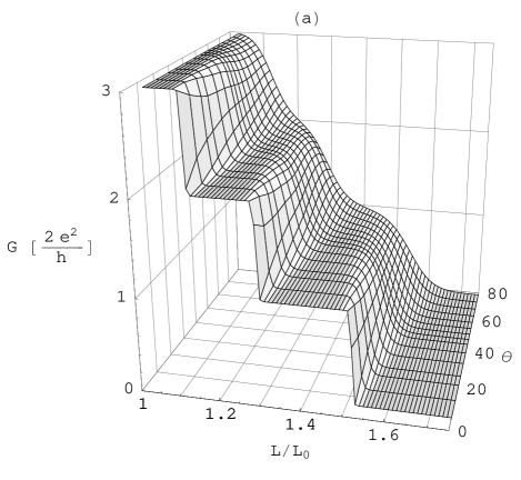
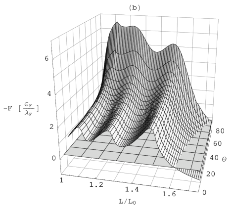
FIG. 3.: Conductance (a) in units of $2e^{2}/h$ and force (b) in units of $\varepsilon_{F}/\lambda_{F}$ as functions of elongation $L/L_{0}$ and opening angle $\theta$ for a fixed width $2k_{F}R=12$.

is independent of the initial length $L_{0}$. We therefore compare in Fig. 2 the analytical results for a single initial length, $k_{F}L_{0}=120$, with numerical results for different $L_{0}$. For $k_{F}L_{0}=120$ the conductance curves are almost indistinguishable, and the numerical result for the force comes very close to the analytically calculated curve. The analytical approach is thus seen to be justified for a long constriction. The behavior for shorter constrictions will be discussed in the next subsection.

An intriguing effect is observed for an elongation $L/L_{0}\gtrsim 1.5$. The force, expected to change sign as soon as the last conductance channel is closed, [3] i.e., for $L/L_{0}\approx 1.5$, is found to remain attractive until $L/L_{0}\approx 1.6$. For the case of gold, this would correspond to a stretching of about $5\AA$ beyond the point where the conductance becomes vanishingly small. This surprising effect may actually have been observed.[1]

We have checked whether this persistent force originates from our arbitrary choice of the shape of the constriction. Therefore, we have determined the shape that minimizes the macroscopic part of the free energy[42] for a fixed elongation. With our constraint, this is equivalent to minimizing the boundary length of the constriction, subject to the condition of constant area. We find that in this case the effect is even stronger than in other geometries. Nevertheless, in three dimensional wires, this persistent force depends strongly on the shape and sometimes even disappears. Further work is needed to clarify the origin of this interesting effect. It is worthwhile to mention that for this optimized shape the conductance steps turn out to be more pronounced and closer to experiments than for other shapes.

B Non-adiabatic constrictions

Our next goal is to go beyond the limitations of the adiabatic approximation and to study short constrictions. To this end, we consider clean systems with a fixed radius $k_{F}R=6$, and vary the initial length $L_{0}$. We characterize the geometry of a wire by its opening angle $\theta$, defined by $\tan\theta=2R/L_{0}$.

In the adiabatic approximation the wavefunction of Eq. (1) is factorized, $\psi(x,z)=\phi^{z}(x)\chi(z)$, and terms containing derivatives of $\phi^{z}(x)$ with respect to $z$ are neglected. This solution corresponds to a set of decoupled channels. In the present context, the approximation is valid if $\left|\frac{1}{r}\frac{dr}{dz}\right|\ll k$, where $k$ is the wave vector of the incident electron. For the case of the conductance, where only states at the Fermi energy are involved, this condition is equivalent to $\theta\ll\pi/2$. Figure 3(a) shows the conductance versus elongation $L/L_{0}$ and opening angle $\theta$. These results for the conductance are consistent with those of Torres et al.:[19] for an adiabatic wire ($\theta\ll\pi/2$), the conductance is well quantized in units of $2e^{2}/h$, with sharp steps between the plateaus, while for non-adiabatic wires the edges are rounded off and the plateaus are no longer well defined. The effects of the geometry on the force are shown in Fig. 3(b). One notices that as $\theta$ increases, the average force becomes larger and the force oscillations are slightly suppressed. The overall increase of the force is due to the increased effect of surface tension in short constrictions. In the two-dimensional case, the surface is one-dimensional, and the surface energy is proportional to the circumference[42]

$$\Omega_{\rm surf}=\frac{2\varepsilon_{F}}{3\lambda_{F}}\partial A=\frac{4\varepsilon_{F}}{3\lambda_{F}}\int_{0}^{L}dz\,\left[1+(dr/dz)^{2}\right]^{1/2}.$$ (12)

In the WKB approximation, the circumference is approximated by $\partial A_{\rm WKB}=2L$, which is a good approximation provided $(dr/dz)^{2}\ll 1$, as pointed out in Ref. [3]. However, this approximation leads to an underestimate of the surface tension in short constrictions, where $|dr/dz|$ is large. The increased effect of surface tension in short constrictions with a special wide-narrow-wide geometry was recently discussed by Kassubek et al.[42] As to the force oscillations, we note that they remain well-defined provided that one can resolve the conductance plateaus. Thus we attribute their decrease with increasing values of $\theta$ to enhanced tunneling.

We remark that wires with larger $\theta$ can be stretched more than ones with small $\theta$, that is to say, the cohesive force remains negative (attractive) further past the point where the conductance goes to zero. Thus the remanent cohesion is enhanced for non-adiabatic constrictions.

C Effects of disorder

We now turn to the study of disorder effects. We first calculate the conductance for a single impurity configuration, then construct histograms from several hundred samples and compare them both with experimental results and previous numerical and theoretical work. Finally, we study the effect of disorder on the tensile force.

1 Conductance for a single impurity configuration

We model an impurity at $\vec{r_{j}}=(x_{j},z_{j})$ by a local potential $V(x,z)=\gamma\delta(x-x_{j})\delta(z-z_{j})$. The disorder for a density $n_{i}$ of impurities can be characterized by the mean free path in the Born approximation, $\ell=\frac{\hbar^{4}k_{F}}{m^{2}n_{i}\gamma^{2}}$. Fig. 4 shows conductance curves for a disordered wire with 7 occupied channels ($k_{F}R=12,\,k_{F}L_{0}=60$), with an impurity concentration $\lambda_{F}^{2}n_{i}=0.27$ both within the constriction and over a length $k_{F}L_{dis}=36$ on each side of the constriction (see Fig. 1). The disorder strengths $\gamma$ correspond to mean free paths in the range $1.2\leq k_{F}\ell\leq 7000$. The spatial distribution of impurities is the same for all curves.

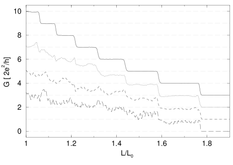
FIG. 4.: Effects of disorder on the conductance of a wire of width $2k_{F}R=24$ and initial length $k_{F}L_{0}=60$. The same configuration of impurities located both within the constriction and in the adjacent regions, as in Fig. 1, is used for each curve. The disordered region is given by $k_{F}L_{dis}=36$, and the impurity concentration is in all cases $\lambda_{F}^{2}n_{dis}=0.27$. The impurity strengths are, from top to bottom, $k_{F}^{2}\gamma=0.29,2.90,7.26\text{ and }21.8\,\varepsilon_{F}$, corresponding, respectively, to mean free paths $k_{F}\ell=7000,70,11\mbox{ and }1.2$. Curves are shifted by one unit of conductance.

For a very large mean free path $k_{F}\ell=7000$ (solid line in Fig. 4), the quantization is almost unaffected by the disorder. When $\ell$ decreases, higher conductance plateaus are destroyed. Lower plateaus remain well defined at first, although they are shifted to lower values (see dotted line in Fig. 4). This shift is smallest for the lowest plateaus. For strong disorder, $k_{F}\ell\approx 1$, the conductance quantization is no longer visible except for the very first step.

This behavior is similar to some experimental results, [9, 22] where only a few conductance steps can be observed, with a shift to conductance values lower than integer multiples of $2e^{2}/h$. This shift is experimentally observed to increase for higher conductance values, in agreement with our numerical results.

2 Conductance histograms

As pointed out by several authors,[11, 22] conductance measurements are reproducible only in very controlled experiments and hence it is easier to study conductance quantization statistically in terms of histograms.[6, 7, 11] In Fig. 5, we show a conductance histogram representing 380 different impurity configurations. The same geometry, impurity concentration, and disorder strength as for the dotted line of Fig. 4 have been used, corresponding to a mean free path $k_{F}\ell=70$. Individual peaks (shown as dotted lines in Fig. 5 ) can be resolved by constructing histograms from partial conductance curves for elongations $L$ in the interval $L_{n+1}<L<L_{n}$, where $L_{n}$ is the midpoint of the $n$-th step of the clean system, i.e. $G(L_{n})=(2e^{2}/h)(n-1/2)$.

FIG. 5.: Conductance histogram made out of 380 individual conductance curves. The width $2R$, initial length $L_{0}$, length $L_{dis}$ and impurity concentration $n_{i}$ are chosen as in Fig. 4. The impurity strength is $k_{F}^{2}\gamma=2.9\,\varepsilon_{F}$ (mean free path $k_{F}\ell=70$). The inset shows the same histogram corrected by the calculated sheet resistance of $R_{s}\simeq 585\,\Omega$.

The peaks of the histogram are not located at integer multiples of $2e^{2}/h$, but are instead shifted to lower values, as is expected from the single curve of Fig. 4. They can be moved back to quantized values of the conductance, as for experimental results,[9] by subtracting a classical resistance in series with that caused by the constriction. This additional contribution can be estimated using the Drude formula for the conductivity, $\sigma=\frac{ne^{2}\ell}{mv_{F}}$, where $n$ is the electronic density. For the mean free path chosen in the simulations we obtain a sheet resistance $R_{s}\simeq 585\,\Omega$. This value of the resistance is consistent with the ones found in experiments (see for example Refs. [8, 9, 10, 11]). Subtracting it from the total resistance, we indeed find that the peaks are shifted to quantized values, as is shown in the inset of Fig. 5.

FIG. 6.: Mean values and widths of the peaks of the conductance histogram of Fig. 5. The bars show the numerical results, while the solid line gives the mean value as predicted from random matrix theory. The dotted line represents the conductance of the clean system and is shown for comparison.

The resolution of individual peaks allows one to calculate the mean value ${\bar{G}_{n}}$ and root-mean-square width $\Delta G_{n}$ of the $n$-th peak. These quantities have been calculated by Beenakker and Melsen using random matrix theory (RMT) for a slightly different situation.[20] They have a set-up where (i) the disordered and constricted parts are spatially separated by scattering-free segments, (ii) the widening between the constricted and unconstricted parts occurs abruptly, and (iii) the disorder is varied, while the constriction remains fixed. In our notation, their results for $n$ open channels are given by

$${\bar{G}_{n}}^{RMT} = \frac{2e^{2}}{h}\left[\frac{n}{1+\gamma_{n}}-\frac{1}{3}\left(\frac{\gamma_{n}}{1+\gamma_{n}}\right)^{3}\right]$$ (13)

$$\Delta G_{n}^{RMT} = \frac{2e^{2}}{h}\left[\frac{2}{15}\left(1-\frac{1+6\gamma_{n}}{(1+\gamma_{n})^{6}}\right)\right]^{1/2}$$ (14)

where $\gamma_{n}=(n+1)\frac{2e^{2}}{h}R_{s}$. These expressions are valid for $\frac{2e^{2}}{h}R_{s}\ll 1$, i.e. for a good conductor. We can mimic the set-up of Ref. [20] by sampling the conductance for elongations corresponding to the midpoints of the plateaus of the clean wire, where tunneling effects are negligible. The width $\Delta G_{n}^{i}$ is then exclusively due to the different impurity configurations. Fig. 6 shows our numerical results (bars), together with the RMT prediction (solid line), calculated from Eq. (13) using the same sheet resistance as in the simulations. The agreement between the mean values is excellent, and the widths, calculated from Eq. (14), deviate less than one percent from the numerical results. This remarkable agreement may be due to the fact that the impurity concentration is low, so that the constriction and the disordered parts are effectively separated by a scattering-free region, as assumed in Ref. [20]. The hypothesis of abrupt widening between the constricted and unconstricted regions appears not to be crucial.

TABLE I.: Comparison of the different widths of the peaks defined in the text

Peak #	$\Delta G_{n}^{tun}$	$\Delta G_{n}^{i}$	$\Delta G_{n}^{RMT}$	$\Delta G_{n}^{tun}+\Delta G_{n}^{i}$	$\Delta G_{n}^{tot}$
1	0.050	0.102	0.105	0.152	0.157
2	0.049	0.149	0.144	0.198	0.205
3	0.045	0.177	0.176	0.222	0.218
4	0.040	0.203	0.203	0.243	0.249
5	0.035	0.226	0.225	0.261	0.257
6	0.028	0.247	0.244	0.275	0.276

The histogram of Fig. 5 also contains a broadening $\Delta G_{n}^{tun}$ due to tunneling, which depends on the shape of the constriction and can be estimated from the results for the clean system. The total widths are found to be well reproduced by simple sums of impurity and tunneling contributions, $\Delta G_{n}^{tot}\approx\Delta G_{n}^{i}+\Delta G_{n}^{tun}$, as shown in Table I.

Finally, we want to emphasize that our result is closer to experiment than previous numerical calculations, [21] in particular with respect to the peak heights, which decrease strongly with increasing conductance. We attribute the improved agreement to the fact that we consider an ensemble of different geometries, with fixed Fermi energy, as in the experiments, while in Ref. [21] the Fermi energy was varied. Since these systems are nearly ballistic, the ergodic behavior[43] expected in the diffusive regime is violated: an ensemble of different geometries with fixed $\epsilon_{F}$ is not statistically equivalent to an ensemble over $\epsilon_{F}$ with fixed geometry.

FIG. 7.: Impurity effects on the tensile force for a wire of width $2k_{F}R=12$, initial length $k_{F}L_{0}=30$ and a disorder characterized by $k_{F}L_{dis}=60$ and $k_{F}\ell=54$ (upper and lower curves). The middle line represents the force of the corresponding clean system.

3 Force

In this last subsection, we study the effects of disorder on the tensile force. In this case, it is no longer optimal to use a delta-function impurity potential. The force appears to be more sensitive to discretization than the conductance. In fact, the lattice constant $a$ must be smaller than the range of the impurity potential. Therefore we use a Gaussian impurity potential with a finite extent $d>a$.

The wire studied has a geometry given by $k_{F}R=6$ and $k_{F}L_{0}=30$. The disordered length is $k_{F}L_{dis}=60$ with an impurity concentration $\lambda_{F}^{2}n_{i}=0.27$, corresponding to a mean free path $\ell=54$. Results are shown in Fig. 7 for two different configurations of disorder. Although the disorder is rather weak, it has a strong effect on the tensile force, and can either weaken or strengthen the cohesion. An intuitive understanding of these opposite behaviors can be obtained by considering the change in the density of electrons due to disorder. An impurity located at the center of the constriction (c.f. upper curve of Fig. 7) would deplete the electron density in the constriction, and thus weaken the cohesion. Correspondingly, impurities located away from the center of the constriction tend to increase the density of electrons in the center, thus increasing the cohesion (c.f. lowest curve of Fig. 7). Further work is needed to understand these effects quantitatively.

V Conclusions

In this paper, we have presented an exact numerical solution of the free-electron model of metallic nanowires,[3] using recursive Green’s function techniques. Our method allows, in principle, to calculate both the conductance and the cohesive properties for wires of arbitrary shape, but for computational reasons we have limited ourselves to two-dimensional wires containing a constriction with a simple geometry.

The validity of the adiabatic and WKB approximations used in Ref. [3] was confirmed for long constrictions, while for short constrictions the cohesion was found to be enhanced. A persistence of the tensile force after closing of the last conducting channel has been observed. It is not yet clear if this is an important physical effect or just a curiosity due to the reduced dimensionality.

We have commonly assumed an ad hoc shape $r(z)$ of the constriction, which in general does not represent equilibrium. A more consistent way would be to calculate the equilibrium shape which minimizes the free energy for a given elongation. We have made a first step in this direction by minimizing the macroscopic part of the free energy. We have found that in this case the wire can be stretched more before it breaks.

Extensive calculations have been made to investigate the effects of random impurities. Our model gives conductance histograms very similar to those observed experimentally. The peaks tend to decrease in height and broaden with increasing conductance. This confirms that disorder in the nanowire is the cause of the resistance that is usually subtracted from experimental results. The positions and widths of the peaks are in excellent agreement with calculations based on random matrix theory.[20] We have shown that the widths have two components, one due to impurities (perfectly described within random matrix theory), the other due to tunneling, which depends on the shape of the constriction.

Our calculations have shown that the effect of disorder is particularly strong on cohesion, which is sensitive to the specific impurity distribution at the center of the constriction. In fact, depending on the presence or absence of an impurity close to the center of the constriction, the cohesion is either decreased or increased. This finding, though qualitatively understandable, requires further study.

Our model may appear to be oversimplified in several respects. We have used hard-wall boundary conditions, neglected both the electron-electron interactions and the ionic background, and assumed a specific geometry upon elongation. However, we do not think that these assumptions are crucial for the essential effects studied in this paper. Other boundary conditions hardly affect the results. Coulomb interactions are found to be barely visible in the cohesion,[31, 32] and are believed to preserve conductance quantization.[44] As to the ionic background, one has to worry on the one hand, about its effects on the electronic structure, and on the other hand, about the kinetics of the deformation. The first effect may produce interesting fine structure in the conductance,[45] while the second can lead to different paths for elongation and contraction processes, [24] explaining the observed hysteresis.[30] A hysteresis effect could be easily reproduced within our model by choosing different geometries for the two processes.

Our approach, where the emphasis is on conduction electrons while the granularity of matter is neglected, is complementary to molecular dynamics simulations, where the atomic rearrangements are followed in detail, while the effects of conduction electrons are taken into account only in an averaged way, e.g. by the embedded atom method. [24] The comparison between our results and experiments shows that, except for hysteresis effects, the overall behavior of both cohesive and electronic properties of metallic nanoconstrictions are well captured by our very simple model.

- [1] G. Rubio, N. Agraït, and S. Vieira, Phys. Rev. Lett. 76, 2302 (1996).
- [2] A. Stalder and U. Dürig, Appl. Phys. Lett. 68, 637 (1996).
- [3] C. A. Stafford, D. Baeriswyl, and J. Bürki, Phys. Rev. Lett. 79, 2863 (1997).
- [4] B. J. van Wees et al., Phys. Rev. Lett. 60, 848 (1988).
- [5] D. A. Wharam et al., J. Phys. C: Solid State Physics 21, L887 (1988).
- [6] L. Olesen et al., Phys. Rev. Lett. 72, 2251 (1994); ibid., 74, 2147 (1995).
- [7] J. M. Krans et al., Nature 375, 767 (1995).
- [8] M. Brandbyge, J. Schiotz, M. R. Sorensen, P. Stoltze, K. W. Jacobsen, and J. K. Norskov, Phys. Rev. B 52, 8499 (1995).
- [9] J. L. Costa-Krämer, Phys. Rev. B 55, R4875 (1997).
- [10] J. L. Costa-Krämer,N. García, P. García-Mochales, P. A. Serena, M. I. Marqués, and A. Correia, Phys. Rev. B 55, 5416 (1997).
- [11] J. L. Costa-Krämer, N. García, and H. Olin, Phys. Rev. B 55, 12910 (1997).
- [12] L. I. Glazman, G. B. Lesovik, D. E. Khmel’nitskii, and R. I. Shekhter, JETP Lett. 48, 238 (1988).
- [13] A. Szafer and A. D. Stone, Phys. Rev. Lett. 62, 300 (1989).
- [14] S. He and S. Das Sarma, Phys. Rev. B 40, 3379 (1989).
- [15] M. Büttiker, Phys. Rev. B 41, 7906 (1990).
- [16] C. W. J. Beenakker and H. van Houten, in Solid State Physics: Advances in Research and Applications, 44, p. 1, H. Ehrenreich and D. Turnbull eds. (Academic Press, New York, 1991).
- [17] D. L. Maslov, C. Barnes, and G. Kirczenow, Phys. Rev. Lett. 70, 1984 (1993); Phys. Rev. B 48, 2543 (1993).
- [18] T. N. Todorov and A. P. Sutton, Phys. Rev. Lett. 70, 2138 (1993).
- [19] J. A. Torres, J. I. Pascual, and J. J. Sáenz, Phys. Rev. B 49, 16581 (1994).
- [20] C. W. J. Beenakker and J. A. Melsen, Phys. Rev. B 50, 2450 (1994).
- [21] P. García-Mochales and P. A. Serena, Phys. Rev. Lett. 79, 2316 (1997).
- [22] M. Brandbyge, K. W. Jacobsen, and J. K. Nørskov, Phys. Rev. B 55, 2637 (1997).
- [23] E. Bascones, G. Gómez-Santos, and J. J. Sáenz, Phys. Rev. B 57, 2541 (1998).
- [24] U. Landman, W. D. Luedtke, N. A. Burnham, and R. J. Colton, Science 248, 454 (1990).
- [25] T. N. Todorov and A. P. Sutton, Phys. Rev. B 54, R14234 (1996).
- [26] U. Landman, W. D. Luedtke, B. E. Salisbury, and R. L. Whetten, Phys. Rev. Lett. 77, 1362 (1996).
- [27] J. M. van Ruitenbeek, M. H. Devoret, D. Esteve, and C. Urbina, Phys. Rev. B 56, 12566 (1997).
- [28] C. Yannouleas and U. Landman, J. Phys. Chem. B 101, 5780 (1997).
- [29] N. W. Ashcroft and N. D. Mermin, Solid state physics (Saunders College Publishing, New York, 1976).
- [30] N. Agraït, G. Rubio, and S. Vieira, Phys. Rev. Lett. 74, 3995 (1995).
- [31] C. Yannouleas, E. N. Bogachek, and U. Landman, Phys. Rev. B 57, 4872 (1998).
- [32] C. A. Stafford, F. Kassubek, J. Bürki, H. Grabert, and D. Baeriswyl, in Quantum Physics at the Mesoscopic Scale, D. C. Glattli and M. Sanquer eds. (Editions Frontières, Gif-sur-Yvette, 1999).
- [33] Y. Kondo and K. Takayanagi, Phys. Rev. Lett. 79, 3455 (1997).
- [34] T. Kizuka, Phys. Rev. B 57, 11158 (1998).
- [35] A. I. Yanson, G. Rubio Bollinger, H. E. van den Brom, N. Agraït, and J. M. van Ruitenbeek, Nature 395, 783 (1998).
- [36] R. Landauer, IBM J. Res. Dev. 1, 223 (1957); Phil. Mag. 21, 863 (1970); D. S. Fisher and P. A. Lee, Phys. Rev. B 23, 6851 (1981); M. Büttiker, Phys. Rev. Lett. 57, 1761 (1986).
- [37] R. Dashen, S.-K. Ma, and H. J. Bernstein, Phys. Rev. 187, 345 (1969).
- [38] V. Gasparian, T. Christen, and M. Büttiker, Phys. Rev. A 54, 4022 (1996).
- [39] E. Akkermans, A. Auerbach, J. E. Avron, and B. Shapiro, Phys. Rev. Lett. 66, 76 (1991).
- [40] A. MacKinnon, Z. Phys. B 59, 385 (1985).
- [41] D. Z. Liu, B. Y.-K. Hu, C. A. Stafford, and S. Das Sarma, Phys. Rev. B 50, 5799 (1994).
- [42] F. Kassubek, C. A. Stafford, and H. Grabert, Phys. Rev. B 59, 7560 (1999).
- [43] P. A. Lee and A. D. Stone, Phys. Rev. Lett. 55, 1622 (1985); B. L. Al’tshuler and B. Z. Spivak, JETP Lett. 42, 477 (1985).
- [44] D. L. Maslov and M. Stone, Phys. Rev. B 52, R5539 (1995); V. V. Ponomarenko, ibid. 52, R8666 (1995); I. Safi and H. J. Schulz, ibid. 52, R17040 (1995); I. Safi, ibid. 55, R7331 (1997); Y. Oreg and A. M. Finkel’stein, ibid. 54, R14265 (1996); R. Egger and H. Grabert, Phys. Rev. Lett. 77, 538 (1996).
- [45] D. Sánchez-Portal, C. Untiedt, J. M. Soler, J. J. Sáenz, and N. Agraït, Phys. Rev. Lett. 79, 4198 (1997).