Determination of optimal effective interactions between amino acids in globular proteins.
(Optimal effective interactions of amino acids)

Abstract

An optimization technique is used to determine the pairwise interactions between amino acids in globular proteins. A numerical strategy is applied to a set of proteins for maximizing the native fold stability with respect to alternative structures obtained by gapless threading. The extracted parameters are shown to be very reliable for identifying the native states of proteins (unrelated to those in the training set) among thousands of conformations. The only poor performers are proteins with heme groups and/or poor compactness whose complexity cannot be captured by standard pairwise energy functionals.

Keywords: potential extraction, fold recognition, optimal stability, energy gap maximization.

1 Introduction

A knowledge of the interaction potentials between amino acids is of crucial importance both for predicting the three-dimensional structure of a protein’s native state and for designing novel proteins, folding on a desired target conformation [BB94, BL91, BL93, CS92, GK92, GL92, SO94, HS95, JT92, OS93, BE94, DA94, KS94, LE76, LE83, SK93, SU93, WU94, DK96, SR95, MS98a, SMM98, CRE, BRTO, AN73]. This builds on the assumption that the interactions between amino acids (and the solvent) are principally responsible for driving the folding of a protein to its native state. This is supported by considerable experimental evidence that the native states of many globular proteins correspond to free energy minima [AN73, WO95, CRE, BRTO].

On a microscopic scale, all-atom potentials are used to carry out “first principle” molecular dynamics for folding [VGUN]. Due to the high level of details included in such calculations, the folding processes of short peptides can be followed only for rather short time-scales (of the order of 1 $\mu$s as in DK98). While the impact of such “ab initio” calculations is destined to grow rapidly, at present, highly satisfactory results can be obtained by adopting mesoscopic phenomenological approaches. Within this framework, a commonly used approach is to avoid a detailed description of an amino acid but represent it as a sphere or an ellipsoid centered on the $C_{\alpha}$ or $C_{\beta}$ position [MC92, SR95, KGS93, SB95, MS98a]. This coarse-grained procedure amounts to integrating out the fine degrees of freedom of a peptide chain and introduces effective interactions between the surviving degrees of freedom.

One commonly used strategy to extract coarse grained potentials between pairs of amino acids has been proposed by MJ85. The method is based on the quasichemical approximation and it entails the calculation of pairing frequencies of amino acids observed in native structures of naturally occurring proteins. Similar approaches have been reviewed by SI95 and WR93. TD96 have recently tested the validity of this procedure on exactly solvable lattice models for proteins. In all the cases they considered the extracted potentials did not correlate too well with the true potentials, although the two sets shared a common trend.

A different strategy for extracting potentials was suggested by MC92 and recently an optimized version has been introduced [VC98, SMB98]. Rigorous tests, similar to the ones in TD96, carried out both for lattice and off-lattice models have shown that the optimized strategy converges to the exact potentials for increasing chain length and/or number of proteins in the training set. The method, explained in detail in section 4, uses the following basic ingredients: the potentials parametrizing a suitably chosen Hamiltonian must be such that the energy of a protein sequence in its own native state is lower than in any other alternative conformations that the protein can attain. For each sequence this yields a set of linear inequalities involving the unknown interaction potentials. Two key points need to be addressed carefully when applying this procedure: the parametrization of the Hamiltonian and the generation of alternative conformations. If the parametrization of the energy is too poor and/or there are unphysical conformations among the decoys (i.e. violating steric contraints), then no consistent solution can be found (unlearnable problem, for an example see VC98 and VN99) . On the other hand, if the parametrization is reliable and there are no unphysical decoy conformations, the energy parameter satisfying the inequalities lie in a convex region of parameter space. While all points inside the cell satisfy the whole set of inequalities, there is an optimal point, typically equidistant from the hyperplanes bounding the cell. The potential parameters corresponding to the optimal point, ensure that the native states of proteins are maximally stable with respect to alternative structures. Our strategy aims at pinpointing the optimal solution, while the original Maiorov and Crippen strategy stopped when reaching an unspecified sub-optimal point inside the cell. Our approach differs from the one employed in [MC92] also because of the different interaction matrix: in our scheme (as in MJ85 or KGS93) the interaction energy of amino acids pairs does not depend on their sequence separation, while a complementary strategy was followed by Maiorov and Crippen. In the next Section we introduce the coarse grained model for proteins and give an overview of the optimal potential extraction technique. The latter is discussed in detail in Section 4. An assessement of the performance of extracted potentials, and a comparison with previously known interactions, are given in Section 3.

2 Theory

2.1 The Model

We choose not to introduce any subdivision of amino acids in classes and retain the full repertoire of 20 types. As is customary, we used a simplified representation of protein structures and replaced amino acids with a centroid placed at the $C_{\beta}$ position [SR95]. A fictitious $C_{\beta}$ was constructed for glycine and for amino acid entries without it, by using standard rotamer angles following PL96.

The basic assumption is that the stable structure of a protein is determined by several factors, that can be ultimately reduced, through an averaging process, to effective contact interactions between amino acids. Thus, we postulate the existence of a functional of the contacts between protein residues, which is in correspondence with the protein energy. The values attained by such a functional should relate to the degree of stability of the conformations housing the sequence.

The strength of a contact between two amino acids whose $C_{\beta}$’s are at positions $r_{1}$ and $r_{2}$ is defined according to the following form, which is a smooth approximation to a stepwise contact function with cutoff at 8.0Å:

$$\Delta(r_{1},r_{2})=\tanh\left(\left(8.0-|r_{1}-r_{2}|\right)/2\right)/2+0.5\ .$$ (1)

The smooth nature of $\Delta(0,r)$ ensures that our results are not very sensitive to the actual form of $\Delta(0,r)$. For simplicity of notation, in the following, we will indicate contact maps with the symbol $\Delta$.

Two Hamiltonian forms for the energy of a sequence $S$ on a structure $\Gamma$ were considered. First we adopted the following contact energy function:

$$E(S,\Gamma)=\sum_{i>j+1}^{N}\epsilon({A_{i}},{A_{j}})\cdot\Delta(r_{i},r_{j})\ ,$$ (2)

where the sum is over all pairs of non-consecutive residues, $N$ is the protein length and ${A_{i}}$ is the amino acid type (there are altogether 20 types) at $r=r_{i}$. $\epsilon$ is the $20\times 20$ matrix of contact energies. Since $\epsilon$ is symmetric, there are only $210$ distinct entries in the matrix. We also considered a second form with 20 additional terms related to the degree of solvation of amino acid types:

$$E(S,\Gamma)=\sum_{i>j+1}^{N}\epsilon({A_{i}},{A_{j}})\cdot\Delta(r_{i},r_{j})+$$

$$+\sum_{i=1}^{N}\epsilon(0,{A_{i}})\cdot\sum_{{\scriptsize\begin{array}[]{c}j=1\\ {j\neq i,i\pm 1}\end{array}}}^{N}\Delta(r_{i},r_{j})\ .$$ (5)

The very last sum in (2.1) corresponds to the total number of contacts of the $i$th residue and reflects its degree of burial. Accordingly, polar amino acids, typically residing at a protein’s surface are expected to have solvation parameters, $\epsilon(0,A)$, larger than the hydrophobic ones. Expression (2.1) is formally equivalent to (2) in that it can be rearranged to obtain a unique sum involving just $210$ terms:

$$E(S,\Gamma)=\sum_{i>j+1}^{N}\left[\epsilon({A_{i}},{A_{j}})+\epsilon(0,{A_{i}})+\epsilon(0,{A_{j}})\right]\cdot\Delta(r_{i},r_{j}).$$ (6)

Nevertheless, using our strategy to extract energy parameters, expressions (2) and (2.1) turn out not to be equivalent. In expression (2.1), the coefficients multiplying $\epsilon(0,A)$ are large with respect to those pertaining to the general $\epsilon(A,A^{\prime})$ entries. The solvation term will accordingly give a significant contribution to the energy of a sequence. This feature was shown to be very useful to discriminate the native state of a protein from decoy structures [PL96, DM97]. Furthermore, by using (2.1), it is possible to estimate the solvent-amino acid interaction, a procedure not carried out by MC92.

The interaction parameters appearing in eq. (2) and (2.1) are not completely independent since the energy scale can be fixed arbitrarily . To remove this degree of freedom, we choose to set the norm of the vector describing the potentials to 1,

$${\sum_{A\leq A^{\prime}}\epsilon^{2}(A,A^{\prime})=1\quad.}$$ (7)

2.2 Optimal strategy

The key prescription at the heart of the potential extraction scheme is that a protein sequence attains the lowest possible energy when mounted on its correct native state. Hence, assuming that the energy parametrizations (2) and (2.1) are reliable, the correct potentials will be such that the native state has the lowest energy when compared to alternative conformations.

The first step of the analysis was to compile a list of non-homologous proteins representing a variety of folds (see section 4 for details). For each protein sequence in this training set, $S_{i}$ (with known native state $\Gamma_{i}$), the alternative structures are obtained by threading on conformations in the training set of equal or longer length [JT92]. Thus, for the correct set of potentials:

$$E(S_{i},\Gamma_{i})<E(S_{i},\Gamma_{D})\ ,$$ (8)

for all the decoy structures, $\Gamma_{D}$, obtained by threading. Therefore, for each sequence in the training set, one obtains an array of inequalities. Due to the finite number of proteins in the training set, the whole ensemble of inequalities will be satisfied by more than a single set of potentials. Indeed, there will typically be a whole region of points in parameter space each corresponding to a set of potentials consistent with inequalities (8). The optimal solution is attained by simultaneously maximizing the stability gap for all proteins in the set. The stability gap is defined as the smallest energy difference between a protein’s native state and one of the decoy conformations. The optimal stability requirement implies that the following inequalities should hold simultaneously for each training protein

$$\frac{E(S_{i},\Gamma_{D})-E(S_{i},\Gamma_{i})}{f\left(D\left(\Gamma_{D},\Gamma_{i}\right)\right)}>c\quad\quad\forall\quad\Gamma_{D}\ ,$$ (9)

where $c$ is a positive quantity to be made as large as possible, the $\Gamma_{D}$’s belong to the set of decoy conformations and the energy interactions satisfy to (7).

The function $f$ in the denominator of (9) is a function of the structural distance between $\Gamma_{D}$ and $\Gamma_{i}$. This serves the purpose of making inequalities (9) more stringent when mounting $S_{i}$ on structurally dissimilar conformations. We used three different trial functions for $f$:

$$f_{1}(x) = 1\ ,$$ (10)

$$f_{2}(x) = x\ ,$$ (11)

$$f_{3}(x) = x^{2}\ .$$ (12)

For the distance function $D(\Gamma,\Gamma^{\prime})$, appearing in eq. (9), we used the Euclidean distance in contact-map space:

$$D\left(\Gamma,\Gamma^{\prime}\right)\equiv\left[\frac{\sum_{i>j+1=2}^{N}(\Delta(r_{i},r_{j})-\Delta(r^{\prime}_{i},r^{\prime}_{j}))^{2}}{(N-1)(N-2)/2}\right]^{1/2}.$$ (13)

$D(\Gamma,\Gamma^{\prime})$ can be viewed as a close relative in terms of contact maps of the standard distance root mean square deviation (DRMSD) but related to our definition of the energy functional.

By threading the training sequences on longer structures, we generated the whole set of inequalities (9). Each of these identifies a hyperplane in parameter space dividing space into two semi-infinite regions; one of which is compatible with the inequality and contains the physical set of parameters [VC98]. When more inequalities are used, the physical region containing the correct parameters reduces to the intersection of all physical hyperspaces. Eventually, the region reduces to a small, convex cell (not necessarily closed) whose walls are determined by a number of inequalities of the order of the dimension of parameter space.

The optimal point in the cell is found by using perceptron strategy, as described in Section 4. This procedure has been shown to converge to the true potential when used in exact models where rigorous test are available [VC98] [CM98]. It is also possible that parametrizations (2) or (2.1) may not be sufficient to guarantee that a solution to inequalities (9) exists. Indeed, if the decoys structures are very competitive with the native structures, three or further body interactions might be necessary to solve inequality (9) consistently [VN99].

This procedure differs significantly from the one of MC92 where the parameters were determined in a sub-optimal manner.

3 Results and discussion

We succeeded in finding an optimal solution to the different systems of inequalities (9): the optimal parameters obtained for Hamiltonians (2.1) and $f=1$ are given in table 1.

We found that only a tiny fraction of all inequalities (9) determine the optimal stability solution (more or less 100 out of 1551196 according to the $f$ used or whether solvation term is present). It is important to ensure that the optimal solution does not fluctuate wildly when stringent inequalities are added or removed. To check this, we eliminated the 100 most stringent inequalities. Even though this completely replaces the walls of the physical cell, the new optimal solution slightly differed from the first one: representing the parameters in a 230-dimensional vector space the two vectors were only $15^{o}$ apart . Such a degree of correlation is significant because the expected angle between two uncorrelated vectors in a space of $\approx 200$ dimensions is about $90^{o}\pm 4^{o}$. This gives confidence in the robustness of the procedure and the statistics of the training set.

The optimal parameters extracted with different trial forms of $f$ in (9) were also closely correlated. As summarized in table 2, their relative angle was always less than $15^{o}$. On the contrary, sub-optimal vectors, for which inequalities (9) are satisfied for $c\approx 0$ (in which case the detailed form of $f$ is not relevant) form, on average, an angle of $50^{0}$ with the optimal solution. This fact underscores the importance of introducing an extremal criterion when maximizing (9).

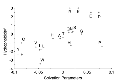
Figure 1: The extracted solvation parameters, $\epsilon(0,A)$ (see eqn. (2.1)) versus standard hydrophobicity values (Creighton 1993, p.154).

The extracted solvation parameters showed a very good correlation (0.67 correlation coefficient) with the hydrophobicity scales as given by CRE. As shown in Fig. 1, the agreement is quite good except, perhaps, for proline. The discrepancy with proline finds a natural explanation within the scheme that we used. In fact, while the hydrophobicity scales in Fig. 1 relate to the propensities of individual, isolated amino acids, the solvation parameter reflects also their structural functionality in a peptide context. In fact, because the prolines are typically located in loop regions, they appear to have an effective hydrophilic propensity larger than their bare value.

Finally, we carried out a stringent validation of the extracted potentials by performing a blind ground-state recognition on a test set. The test set (see Table 3)was comprised of proteins taken from those used in MJ96 and chosen so that they would meet some of the criteria used to select the training set (see section 4). We deliberately introduced proteins with hetero groups, low degree of compactness and also pairs with high structural homology. In all cases we ensured that no protein in the test set had a significant degree of structural homology with those in the training one.

We took, in turn, the sequences of the test set and threaded them on structures in the set with equal or longer length. Hence, we checked whether using the optimal potential parameters of Table 1, the true native state was recognized as the lowest energy one. Indeed, this turned out to be the case for all but 6 proteins. No higher success rate was found on using some other known sets of potentials consistent with the form of our Hamiltonian.

Another relevant quantity related to the performance of the algorithm is given by the number of wrongly satisfied inequalities of type (9) for the test set. This quantity shows a much higher degree of variability than the number of correctly identified ground states and is given in column 3 of Table 4. It can be seen that the optimal parameters extracted with the solvent and $f=1$ perform far better than those without the solvent and previously extracted ones. It also appears that, enforcing optimality provides a dramatic reduction of wrong inequalities compared to the sub-optimal cases. This provides a sound a posteriori justification for the optimal extraction procedure as well as giving confidence in the parameters.

The few cases where the extracted potentials fail are due to one of the following situations: a) the native protein is not too compact or b) it contains stabilizing hetero groups. Situations in which a highly homologous structure has a lower energy score than the native one are not deemed as errors. A typical energy/structural distance plot is shown in Fig. 5. It is apparent that homologous structures have energies similar to that of native conformations, while distant structures lie higher in energy. Some differences in the performance were observed for the sets of 210 and 230 potentials. While the latter only fail to recognize native states containing heme groups etc., the former occasionally fail to recognize the native states with no atypical feature (e.g. interleukin-4, 1rcb).

For proteins with heme groups, several structures score better: they usually present a smaller number of contacts than the native structure being less compact than the native state. This is possibly related to the presence of proline in an unusually buried position, namely the heme pocket. In fact, due to the high effective solvation term assigned to proline, the native structure is penalized with respect to decoy ones where it is confined in more solvent-exposed positions.

An interesting case where the failure relates to a non-compact protein, is given by trp aporepressor (3wrp), for which several better scoring decoys exist. The explanation lies in the fact that 3wrp is always found as a dimer: the side of the protein binding its counterpart has non-polar surface residues usually in contact with non-polar residues on the other dimer, which is not accounted for by our procedure.

Nevertheless, the algorithm appears to work in other instances of non-compact conformations such as troponin c (4tnc) and calmodulin (1cll) and on some cytochrome-c as 1ccr or 1yeb, showing that the optimization procedure succeeds in extracting a potential with a wider applicability range than that given by the folds used in the training set.

Over 15 different pairs of homologous structures (contact map distance less than 0.1), the energy functional is able to rank the true native state as the lowest in just 8 cases. In the other cases the native state attains an energy value slightly higher than the homologous one. As expected, the simple contact potential cannot distinguish the native state among very similar structures but it consistently assigns similar value of energy to similar conformations according to the degree of similarity (see Fig. 5).

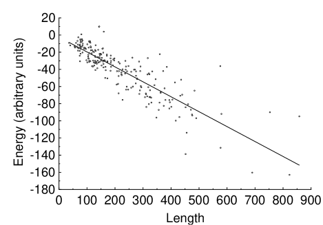
Figure 6: When using the extracted parameters of Table 1 the native state energy of proteins shows an approximately linear behavious as a function of their length. Points refer to proteins for both the training and test sets. Proteins with less than 200 amino acids and atypical compactness present significant deviations from the average trend.

It is important to note that there is a well-defined trend for the protein ground-state energies as a function of protein length. Deviations from this typical trend could be used to assess the reliability of the predicted fold of a sequence with unknown structure (Fig. 6).

4 Methods

4.1 Protein data sets

We selected 142 protein structures from PDB [PDB], listed in Tab. LABEL:training.table, with lengths varying from 36 to 823, following criteria very similar to MC92. For each reference protein, we built a set of alternative conformations by threading its sequence on all the other structures in the set with a greater or equal number of amino acids. As explained in JT92, threading a sequence of $L$ amino acids on a structure, $\Gamma^{\prime}$, of length $L^{\prime}>L$, involves mounting the sequence on all the ($L^{\prime}-L+1$) segments (of contiguous amino acids) taken from $\Gamma^{\prime}$. This procedure assigns the contact map of the threaded segment to the threading sequence. The inherited contact map is used to calculate the energy of the sequence in the alternative, threaded, conformation, and compared with the energy in its native state, which is required to be the global energy minimum.

Only single chain structures have been selected in order to avoid the occurrence of interchain contacts between amino acids, that are not detected by our procedure and that could cause the stabilization of hydrophobic residues on a protein’s surface. Considering multiple chain structures would have introduced spurious effects in the extracted potentials, since inter-chain contacts would not be present in threaded conformations. For simplicity, however, we decided to retain proteins which may be found in polymeric forms. Because the presence of large hetero groups can distort the usual geometry of dihedral angles between amino acids and cannot be treated in a simple way by a pairwise potential, we discarded protein structures with high percentages of non-water HETATM records in their PDB files (like HEM or CPS groups).

We used the classification of 3-D protein structures SCOP [MB95] to select proteins spanning a wide range of different three dimensional folds: no pair of proteins in our training set belong to the same SCOP family. Furthermore, we have included only proteins in the first 4 SCOP classes: all-$\alpha$, all-$\beta$, $\alpha$/$\beta$ and $\alpha+\beta$ proteins. Cell membrane or surface proteins and very short peptide chains are excluded because usually they are not stabilized by just amino acid interactions but by some external factors, such as the hydrophobic environment, metal ligands, heme groups etc. No unresolved backbone atoms inside a chain are allowed; disordered or unresolved terminal backbone atoms are eliminated.

We also disregarded proteins that were not typically compact: because there is a clear dependence of the radius of gyration and the number of contacts among amino acids on chain length, we rejected from our training set proteins with too large a radius of gyration or with significantly fewer contacts than expected for their length. The rejection was based using the quantitative procedures discussed in MC92.

4.2 Optimal Stability Perceptron

It is convenient to recast expression (9) so that the dependence from the interaction parameters between amino acid types $A$ and $A^{\prime}$, $\epsilon(A,A^{\prime})$ appears explicitly,

$$\sum_{\it{A}\leq A^{\prime}}\frac{\epsilon(A,A^{\prime})}{|\vec{\epsilon}|}\cdot\frac{n_{S_{i},\Gamma_{D}}(A,A^{\prime})-n_{S,\Gamma_{i}}(A,A^{\prime})}{f\left(D(\Gamma_{D},\Gamma_{i})\right)} > c\ .$$ (14)

where $n_{S,\Gamma}(A,A^{\prime})$ is the number of contacts between amino acids $A$ and $A^{\prime}$ attained by $S$ on $\Gamma$. The indices $A$ and $A^{\prime}$ run over the 20 amino acid classes for parametrization 2. Expression 14 can be rewritten in a more compact form by mapping the independent entries of the $\epsilon$ matrix on a one-dimensional vector,

$$\vec{\epsilon}\equiv\{\epsilon(1,1),\epsilon(1,2),...,\epsilon(20,20)\}\ .$$ (15)

and likewise for the vector

$${\vec{N}_{S,\Gamma,\Gamma^{\prime}}\equiv\{\frac{(n_{S,\Gamma}(1,1)-n_{S,\Gamma^{\prime}}(1,1))}{f\left(D(\Gamma^{\prime},\Gamma)\right)},...\}/.}$$ (16)

With the former definitions, equation (11) becomes:

$$\frac{\vec{\epsilon}}{|\vec{\epsilon}|}\cdot\vec{N}_{S_{i},\Gamma_{i},\Gamma_{D}}>c\ .$$ (17)

A formally equivalent expression is obtained when using 230 parameters as in eq. (2.1).

Expression (17) leads to a geometrically appealing interpretation of the stability requirement. The optimal stability is reached when the interaction vector has the largest possible inner product with all the $\vec{N}_{S_{i},\Gamma_{i},\Gamma_{D}}$ vectors, also termed “patterns”, originated from the training set. A rigorous solution for this geometrical problem was given by KM87 who suggested an iterative procedure called optimal stability perceptron.

The procedure is the following. Starting from a random (or an otherwise assigned) set of interactions satisfying the norm constraint (7), the stability score of all inequalities is computed. Then, the potentials are updated so to increase the stability of the lowest scoring inequality. This is done by adding to the original potentials vector, $\vec{\epsilon}$, a small term proportional to the worst scoring pattern (see Fig. 2):

$$\forall A,A^{\prime}\quad\epsilon(A,A^{\prime})\rightarrow\epsilon(A,A^{\prime})+\frac{1}{d}N_{S,\Gamma,\Gamma^{\prime}}(A,A^{\prime})\ ,$$ (18)

where $d$ is the dimension of the parameter space (210 or 230). Then, the inequalities are re-computed with the updated interaction parameters. The lowest scoring one is identified again and a new update of $\vec{\epsilon}$ is carried out. Note that the update (18) will typically change the norm of $\vec{\epsilon}$. The unit norm (see eqn. (7)) can be conveniently enforced after convergence has been achieved.

While convergence is guaranteed to be reached in a finite number of steps, the time required for each iteration grows linearly with the number of inequalities. In our case, we typically dealt with $\approx 10^{6}$ inequalities, and convergence sometimes required several thousand iterations (each taking few seconds of CPU time). Hence, we devised a scheme to speed up convergence based on the observation that the stability variation due to the change of parameters is proportional to the distance between the inequality point and the parameter direction,

$$\Delta s= \vec{N}\cdot\Delta\vec{\epsilon}=\vec{N}_{\perp\vec{\epsilon}}\cdot\Delta\vec{\epsilon}_{\perp\vec{\epsilon}}+\underbrace{\vec{N}_{\parallel\vec{\epsilon}}\cdot\Delta\vec{\epsilon}_{\parallel\vec{\epsilon}}}_{\geq 0.0}\propto$$ (19)

$$\propto\underbrace{a}_{\not=0.0}\cdot|\vec{N}_{\perp\vec{\epsilon}}|+\underbrace{b}_{\geq 0.0} \ .$$

This implies that inequality vectors far from the parameter direction will get the largest score variations (positive or negative) and so they are more likely to become the lowest scoring ones. Accordingly, the standard perceptron procedure was run until reaching a sub-optimal value for the stability threshold, $c>0$; this typically needed 300 iterations. Then we temporarily restricted the updating procedure to those inequalities lying outside a cone with axis along the parameter direction and vertex at distance larger than $c$ from origin (see Fig. 3 ). The cone width was determined to limit the number of inequalities to less than $20000$ (Fig. 3). In this way we had to deal with $10^{4}$ inequalities that are 2 orders of magnitude smaller than the original ones, thus decreasing enormously the CPU time needed for optimization. Furthermore, after convergence, the neglected inequalities are found to be satisfied well above the optimal stability threshold $c_{max}$, thus justifying the numerical shortcut.

We conclude by remarking that, if the relative correction to $\epsilon(A,A^{\prime})$ in eq. (18) is too large, this may result in a slowing down of the convergence. This difficulty can be readily circumvented by increasing the size of $\vec{\epsilon}$ by an order of magnitude. It was typically necessary to repeat this “inflation” procedure 3-4 times during each run towards convergence (see Fig. 4). This was sufficient to reach optimal convergence to the solution: $\Delta c/c<10^{-}3$.

Acknowledgments. We acknowledge support from INFM, NASA, NATO and the Petroleum Research Fund administered by the American Chemical Society. We thank C. Clementi, R. Dima, L. Guidoni, S. Piana, A. Rossi, F. Seno and J. Van Mourik for useful discussions.

A	-0.0269
C	-0.0142	-0.1509
D	0.0222	0.0027	-0.0130
E	0.0308	0.0047	0.1587	0.0712
F	0.1415	-0.0500	0.0167	0.0458	-0.1098
G	0.0386	0.0635	-0.0015	0.0205	-0.0774	0.0023
H	0.0392	-0.0293	0.0255	-0.0472	0.0240	-0.0322	0.0046
I	-0.0261	-0.0960	0.1188	0.1026	-0.0423	0.0310	0.0175	-0.1753
K	0.0760	0.0372	-0.0675	-0.2113	0.0302	-0.0050	0.0137	0.1177	0.0498
L	-0.0540	0.0776	0.0078	0.0740	-0.0988	-0.0787	0.0849	-0.0672	-0.0431	-0.1246
M	0.0070	0.0239	-0.0995	0.0116	-0.0614	-0.0241	-0.0603	-0.0472	0.0807	0.0179	0.0393
N	0.0036	-0.0158	0.0208	-0.1343	0.1070	0.0377	-0.0005	0.1172	-0.0636	0.1172	-0.0070	-0.0064
P	-0.0760	0.0134	0.0180	0.0272	0.1145	-0.0043	0.0615	0.0253	-0.0798	0.0125	-0.0205	0.0713	0.0381
Q	-0.1203	0.0294	0.0724	0.0274	0.0853	0.0527	-0.0068	0.0530	-0.0691	-0.0792	0.0176	-0.0199	-0.0460	0.0141
R	0.0154	0.0202	-0.1486	-0.1610	-0.1207	-0.0010	-0.0315	0.0528	0.0892	-0.1136	0.0646	0.0225	-0.0228	0.0233	0.0624
S	0.0358	0.0047	-0.1300	-0.0895	0.0580	-0.0257	-0.0469	0.0288	0.0214	0.2016	-0.0236	-0.1070	0.0085	0.0671	0.0733	-0.0618
T	-0.0831	-0.0511	-0.0687	0.1258	-0.0492	0.0526	-0.0890	-0.0541	0.0180	0.1139	0.0914	-0.1003	0.0623	0.0087	0.0340	-0.0576	0.0138
V	-0.0658	-0.0066	0.0702	-0.0609	-0.0185	-0.0406	0.0911	-0.0908	-0.0146	-0.0724	0.0465	0.0365	-0.0351	-0.0155	0.0528	0.0927	0.0414	-0.0637
W	0.0878	0.0129	0.0575	0.0093	0.0210	0.0055	0.0123	-0.0631	0.0281	0.0058	0.0380	-0.0487	-0.0345	-0.0733	0.0007	-0.0076	0.0234	-0.0504	0.0118
Y	-0.0367	0.0389	0.0111	0.0521	-0.1059	0.0249	-0.0507	-0.0505	0.0235	-0.0265	-0.0785	-0.0117	-0.0536	-0.0089	0.1021	-0.0219	-0.0317	0.0482	-0.0826	0.1660
Sol	-0.0053	-0.0850	0.0737	0.0575	-0.0901	0.0387	-0.0201	-0.0478	0.0317	-0.0448	0.0164	0.0186	0.0801	0.0121	0.0141	0.0202	0.0006	-0.0556	-0.0462	-0.0923
	A	C	D	E	F	G	H	I	K	L	M	N	P	Q	R	S	T	V	W	Y

Table 1: Interaction parameters extracted by using energy funtional  (2.1).

Solvent
$f=1$	$f=x$	$10.1^{o}$
$f=1$	$f=x^{2}$	$13.5^{o}$
$f=x$	$f=x^{2}$	$6.67^{o}$
$f=1$	Non-optimal	(average) $54^{o}$
$f=x$	Non-optimal	(average) $55^{o}$
$f=x^{2}$	Non-optimal	(average) $55^{o}$
Non-optimal	Non-optimal	(average) $67^{o}$
No-Solvent
$f=1$	$f=x$	$8.5^{o}$
$f=1$	$f=x^{2}$	$15.9^{o}$
$f=x$	$f=x^{2}$	$10.0^{o}$

Table 2: Angles formed by the optimal vectors for various forms of the Hamiltonian and $f$ (see eqns. (2), (2.1) and (9).

Prot. code	Length	Native Energy	No. Decoys	No. Better Str.	Average	SCOP
					Difference	Classification
					in Contacts
1hbg	146	-23.259936	8007	0	0 $\pm$ 0	1001001001001	003
1mba	146	-22.890319	8007	0	0 $\pm$ 0	1001001001001	005
1mbs	151	-22.674067	7756	0	0 $\pm$ 0	1001001001001	006
1lh1	152	-35.490600	7707	0	0 $\pm$ 0	1001001001001	014
2lhb	149	-21.766920	7855	0	0 $\pm$ 0	1001001001001	033
1cty	108	-7.089541	10259	5	-57 $\pm$ 81	1001003001001	004
1yeb	108	-7.110300	10259	$1^{\dagger}$	-3 $\pm$ 0	1001003001001	004
1ccr	111	-7.226756	10056	0	0 $\pm$ 0	1001003001001	006
2c2c	112	-8.985422	9989	2	-150 $\pm$ 170	1001003001001	009
351c	82	-4.752413	12127	3	17 $\pm$ 50	1001003001001	017
$\star$ 1le4	139	-25.618122	8383	0	0 $\pm$ 0	1001023001001	003
2mhr	117	-21.248559	9670	0	0 $\pm$ 0	1001023004001	004
1rcb	129	-30.026804	8944	0	0 $\pm$ 0	1001025001002	002
$\star$ 4tnc	160	3.959946	7332	0	0 $\pm$ 0	1001034001005	001
$\star$ 1cll	143	9.773591	8166	0	0 $\pm$ 0	1001034001005	005
$\star$ 1clm	144	9.950750	8112	1	-370 $\pm$ 0	1001034001005	011
1cca	291	-36.626670	2654	0	0 $\pm$ 0	1001065001001	003
$\star$ 3wrp	101	-10.772739	10755	9	235 $\pm$ 90	1001078001001	001
1poc	134	-31.651214	8659	0	0 $\pm$ 0	1001095001001	001
2imm	114	-17.753696	9858	0	0 $\pm$ 0	1002001001001	024
2rhe	114	-14.557044	9858	0	0 $\pm$ 0	1002001001001	088
2stv	184	-27.148904	6318	0	0 $\pm$ 0	1002008001002	002
2cna	237	-30.109204	4302	0	0 $\pm$ 0	1002019001001	001
1lec	242	-60.150421	4129	0	0 $\pm$ 0	1002019001001	004
1lte	239	-36.671976	4231	0	0 $\pm$ 0	1002019001001	005
1shg	57	-14.578324	14051	0	0 $\pm$ 0	1002021002001	006
8adh	374	-82.544846	1113	0	0 $\pm$ 0	1002022001002	001
1gbt	223	-43.532366	4821	0	0 $\pm$ 0	1002031001002	001
1est	240	-63.644775	4196	0	0 $\pm$ 0	1002031001002	013
4ape	330	-78.686637	1763	0	0 $\pm$ 0	1002034001002	001
3app	323	-72.409291	1897	0	0 $\pm$ 0	1002034001002	002
2apr	325	-64.356790	1856	0	0 $\pm$ 0	1002034001002	003
3pep	326	-72.156108	1836	0	0 $\pm$ 0	1002034001002	006
1mpp	356	-87.210810	1356	0	0 $\pm$ 0	1002034001002	009
1cms	321	-80.466445	1940	0	0 $\pm$ 0	1002034001002	011
1brp	173	-30.565982	6770	0	0 $\pm$ 0	1002041001001	002
1mup	157	-30.854982	7471	0	0 $\pm$ 0	1002041001001	008
2aaa	475	-92.682878	340	$1^{\dagger}$	37 $\pm$ 0	1002048001001	008
6taa	476	-93.727839	335	0	0 $\pm$ 0	1002048001001	009
1btc	490	-96.939667	292	0	0 $\pm$ 0	1003001001002	001
1ald	363	-67.400922	1257	0	0 $\pm$ 0	1003001003001	002
3enl	436	-52.025765	553	0	0 $\pm$ 0	1003001006001	001
1pii	452	-138.741679	456	0	0 $\pm$ 0	1003001008001	001
1xis	385	-37.102765	980	0	0 $\pm$ 0	1003001012001	004
1phh	394	-85.545211	880	0	0 $\pm$ 0	1003004001002	002
1gal	580	-91.922051	111	0	0 $\pm$ 0	1003004001002	004
1dhr	236	-44.849628	4339	0	0 $\pm$ 0	1003019001002	006
2cmd	312	-83.791376	2147	0	0 $\pm$ 0	1003019001005	002
1ldm	329	-73.012055	1781	0	0 $\pm$ 0	1003019001005	008
1gky	186	-30.194166	6237	0	0 $\pm$ 0	1003025001001	001
3adk	194	-28.274731	5924	0	0 $\pm$ 0	1003025001001	006
121p	166	-37.077357	7067	$1^{\dagger}$	84 $\pm$ 0	1003025001003	001
4q21	167	-40.978706	7023	0	0 $\pm$ 0	1003025001003	001
1sbc	274	-56.392841	3113	0	0 $\pm$ 0	1003028001001	001
1thm	279	-51.381279	2968	0	0 $\pm$ 0	1003028001001	003
1s01	275	-47.482543	3082	0	0 $\pm$ 0	1003028001001	006
1s02	275	-42.291256	3082	$1^{\dagger}$	3 $\pm$ 0	1003028001001	006
2prk	279	-50.558910	2968	0	0 $\pm$ 0	1003028001001	007
1ama	401	-83.687554	813	0	0 $\pm$ 0	1003048001001	001
1spa	396	-78.338515	859	0	0 $\pm$ 0	1003048001001	004
1ipd	345	-51.476690	1522	0	0 $\pm$ 0	1003057001001	001
3icd	414	-55.210210	708	0	0 $\pm$ 0	1003057001001	003
1rhd	292	-59.479630	2628	0	0 $\pm$ 0	1003060001001	001
3pfk	319	-60.742159	1985	0	0 $\pm$ 0	1003070001001	002
1ovb	159	-37.670779	7378	0	0 $\pm$ 0	1003073001002	002
1lfg	690	-160.321444	0	0	0 $\pm$ 0	1003073001002	005
132l	129	-32.386126	8944	$1^{\dagger}$	14 $\pm$ 0	1004002001002	001
1lz3	129	-32.719245	8944	0	0 $\pm$ 0	1004002001002	002
1laa	130	-40.734890	8884	0	0 $\pm$ 0	1004002001002	008
1alc	121	-36.611850	9425	0	0 $\pm$ 0	1004002001002	013
3il8	68	-18.129049	13192	0	0 $\pm$ 0	1004007001001	001
1fkb	106	-14.625747	10399	0	0 $\pm$ 0	1004019001001	001
1yat	113	-13.260539	9923	0	0 $\pm$ 0	1004019001001	003
1ctf	68	-11.121616	13192	0	0 $\pm$ 0	1004026001001	001
1fd2	106	-27.581742	10399	0	0 $\pm$ 0	1004033001002	001
2fxb	81	-7.781913	12202	0	0 $\pm$ 0	1004033001004	003
3tms	264	-60.007310	3424	0	0 $\pm$ 0	1004063001001	001
3b5c	84	-12.241707	11980	0	0 $\pm$ 0	1004066001001	001

Table 3: Proteins used in the test set. The symbol $\dagger$ denotes instances where the better scoring structure is homologous to the target protein, while a $\star$ marks non compact native state. 1lfg has been used only as structural template.

	Score on Test
Solvent	Not Rec. Str.	Unsat. Ineq.
$f=1$	5	25
$f=x$	5	33
$f=x^{2}$	5	36
Non-Optimal	5.25	75.7
No Solvent
$f=1$	6	118
$f=x$	6	200
$f=x^{2}$	6	254
DBMS	7	51
KGS	6	452
MC	6	48
	Score on Training
DBMS	13	1091
KGS	22	9789
MC	20	1826

Table 4: Performance of the potentials extracted in this work and other known sets. The second column gives the number of unrecognised native states among the 78 ones of Table LABEL:training.table. The associated number of violated inequalities (against a total of 444199) is given in column 3. The acronyms for the alternative potentials refer to: DBMS$=$(Dima et al. 1999), KGS$=$(Kolinsky et al. 1993), MC$=$(Maiorov & Crippen 1994). The last part of the table shows the scores of the alternative potentials applied to our training set of 142 proteins generating 1551196 inequalities (on which our potentials, by definition, scores 100% success).

Table 5: List of “training proteins” used to extract interaction potentials.

Prot. Code	Length	SCOP Classification		No. Decoys
1vii	36	1001014001001	001	25461
1erd	40	1001010001001	002	24896
1pru	56	1001030001003	001	22655
1fxd	58	1004033001001	001	22376
1igd	61	1004012001001	001	21961
1orc	64	1001030001002	005	21549
1sap	66	1004009001001	002	21276
1mit	67	1004022001001	003	21140
1utg	69	1001072001001	001	20871
1ail	70	1001015001001	001	20737
1hoe	74	1002004001001	001	20208
1kjs	74	1001040001001	001	20208
1ubi	74	1004012002001	001	20208
1hyp	75	1001042001001	001	20076
5icb	75	1001034001001	001	20076
1fow	76	1001004004001	001	19947
1tif	76	1004012006001	001	19947
1tnt	76	1001006001001	001	19947
1acp	77	1001026001001	001	19820
1hdj	77	1001002002001	001	19820
1iba	77	1004053001001	001	19820
1vcc	77	1004067001001	001	19820
1coo	81	1001032001001	001	19336
1cei	84	1001026002001	001	18978
1ngr	84	1001062001001	001	18978
1opd	85	1004052001001	003	18859
1fna	90	1002001002001	002	18278
1hqi	90	1004079001001	001	18278
1who	94	1002006003001	001	17820
1pdr	96	1002023001001	001	17593
1beo	98	1001096001001	001	17368
1tul	101	1002060004001	001	17034
9rnt	104	1004001001001	003	16703
1aac	105	1002005001001	001	16593
1erv	105	1003033001001	004	16593
1jpc	108	1002054001001	001	16270
1kum	108	1002003001001	005	16270
1rro	108	1001034001004	001	16270
3ssi	108	1004044001001	002	16270
2mcm	112	1002001006001	001	15854
1mai	118	1002037001001	001	15241
1poa	118	1001095001002	001	15241
1whi	122	1002025001001	001	14839
1yua	122	1004067001002	001	14839
7rsa	124	1004004001001	001	14641
2phy	125	1004061002001	001	14543
1bfg	126	1002028001001	001	14446
3chy	128	1003013002001	001	14255
1pdo	129	1003040001001	001	14160
1tum	129	1004062001001	001	14160
1ifc	131	1002041001002	002	13974
1kuh	131	1004050001001	001	13974
1lis	131	1001017001001	001	13974
1rsy	132	1002006001002	001	13882
1cof	135	1004060001002	001	13617
2end	137	1001016001001	001	13442
5nul	138	1003013004001	006	13355
2sns	140	1002026001001	001	13184
1lcl	141	1002019001003	004	13099
1lba	145	1004064001001	001	12766
1pkp	145	1004011001001	002	12766
1vsd	145	1003041003002	001	12766
1npk	150	1004033006001	002	12363
1irp	153	1002028001002	003	12125
2rn2	155	1003041003001	001	11968
1vhh	157	1004034001002	001	11813
1gpr	158	1002059003001	001	11736
1ra9	159	1003053001001	001	11660
119l	162	1004002001003	001	11437
2cpl	164	1002043001001	001	11290
1sfe	165	1001004002001	001	11217
1wba	171	1002028003001	001	10790
2fha	171	1001024001001	003	10790
1amm	173	1002009001001	001	10650
2prd	173	1002026005001	003	10650
1ido	184	1003045001001	002	9911
153l	185	1004002001004	001	9844
1xnb	185	1002019001008	001	9844
1knb	186	1002016001001	001	9778
1kid	192	1003005003001	001	9399
1cex	197	1003013007001	001	9088
1chd	198	1003027001001	001	9026
1fua	206	1003055001001	001	8545
1thv	207	1002018001001	001	8485
2abk	211	1001066001001	001	8252
1ah6	213	1004068001001	001	8137
1lbu	213	1001019001001	001	8137
3cla	213	1003030001001	001	8137
2ayh	214	1002019001002	002	8080
1gpc	217	1002026004007	003	7920
1akz	223	1003011001001	001	7607
1dad	224	1003025001005	001	7555
1aol	227	1002015001001	001	7404
1cby	227	1004058001001	001	7404
1lbd	238	1001087001001	001	6874
2baa	243	1004002001001	001	6638
1mrj	247	1004094001001	001	6453
3fib	248	1004098001001	001	6407
1plq	258	1004076001002	001	5966
2cba	258	1002050001001	002	5966
1arb	262	1002031001001	001	5796
1ako	268	1004086001001	001	5549
2dri	271	1003072001001	001	5428
1tml	286	1003002001001	001	4842
1han	287	1004020001003	002	4803
1nar	289	1003001001005	002	4728
1amp	290	1003052003004	001	4691
1ctt	294	1003075001001	001	4550
2ctc	307	1003052003001	001	4107
1ede	310	1003050001003	001	4007
1pgs	311	1002011001001	001	3974
1ads	315	1003001005001	002	3849
1hyt	316	1001053001001	002	3818
1tca	317	1003050001007	001	3788
1pot	321	1003073001001	011	3675
1axn	323	1001051001001	001	3620
1dxy	329	1003013009001	002	3463
1nif	333	1002005001003	001	3362
1rpa	341	1003043001002	001	3169
1uby	348	1001091001001	001	3007
1idk	359	1002056001002	001	2764
1eur	360	1002045001001	004	2742
1cem	363	1001073001002	001	2681
1pud	372	1003001017001	001	2509
1kaz	377	1003041001001	001	2418
1edg	380	1003001001003	002	2366
1php	394	1003066001001	003	2141
1phc	405	1001075001001	001	1975
1uae	417	1004035002001	001	1806
1gnd	430	1003004001003	001	1636
1csh	433	1001074001001	001	1599
1pmi	440	1002058002001	001	1521
1gcb	452	1004003001001	008	1400
2bnh	456	1003007001001	001	1363
3grs	461	1003004001004	001	1322
1gai	471	1001073001001	001	1251
1lam	484	1003036001001	001	1172
1vnc	576	1001080001001	001	711
1ciy	577	1002013001002	002	706
1amj	753	1003005002001	002	177
1gpb	823	1003068001002	001	36
1qba	858	1002001001005	002	0

Figure 2: Schematic representation of a typical perceptron update in a two-dimensional space. Inequalities are represented by vectors connecting the origin to the points. At ineration $n$, The stability, $c$, of ineq. (9) is the smallest inner product between the parameter vector $\vec{\epsilon}_{n}$ and each of the inequalities. In case (a) $c$ is given by $\vec{\epsilon}\cdot\vec{N}$ and $\vec{\epsilon}_{n}$ accordingly aquires a small component parallel to $\vec{N}$. An equilibrium situations is shown in (b). Successive updates cause $\vec{\epsilon}$ to bounce on either side of the equilibrium direction. The latter is reached in a finite time, because the relative size of the added component decreases with the number of iterations.

Figure 3: After a sufficient number of iterations, successive perceptron updates will not change appreciably $\vec{\epsilon}$. To speed up convergence, it is convenient to temporarily retain only those inequalities (points in parameter space) lying outside a cone with axis along $\vec{\epsilon}$ and suitable vertex and width (see text). The edge of the cone is visible in this figure, where only the retained inequalities are shown.

Figure 4: Perceptron stability as a function of the number of iterations. The discontinuities are associated with the “inflation” of $\vec{\epsilon}$ used to speed up convergence (see text).

Figure 5: Energies of the protein sequence 1lz3 when threaded on decoy structures against structual dissimilarity. Very low energies are observed when threading on homologous conformations (in particular protein 132l).

References

- [1] \harvarditemAnfinsen1973AN73 Anfinsen, C. \harvardyearleft1973\harvardyearright. Principles that govern the folding of protein chains, Science 181: 223–239.
- [2] \harvarditemBauer \harvardand Beyer1994BB94 Bauer, A. \harvardand Beyer, A. \harvardyearleft1994\harvardyearright. An improved pair potential to recognize native protein folds, Proteins: Structure Function and Genetics 18: 254–261.
- [3] \harvarditem[Bernstein et al.]Bernstein, Koetzle, Williams, Meyer, Brice, Rodgers, Kennard, Shimanouchi \harvardand Tasumi1977PDB Bernstein, F., Koetzle, T., Williams, G., Meyer, E. J., Brice, M., Rodgers, J., Kennard, O., Shimanouchi, T. \harvardand Tasumi, M. \harvardyearleft1977\harvardyearright. The protein data bank: a computer-based archival file for macromolecular structures, J. Mol. Biol. 112: 535–542.
- [4] \harvarditemBowie \harvardand Eisenberg1994BE94 Bowie, J. \harvardand Eisenberg, D. \harvardyearleft1994\harvardyearright. An evolutionary approach to folding small -helical proteins that uses sequence information and an empirical guiding fitness function, Proc. Natl. Acad. Sci. USA 91: 4436–4440.
- [5] \harvarditem[Bowie et al.]Bowie, Lüthy \harvardand Eisenberg1991BL91 Bowie, J., Lüthy, R. \harvardand Eisenberg, D. \harvardyearleft1991\harvardyearright. A method to identify protein sequences that fold into a known three-dimensional structure, Science 253: 164–170.
- [6] \harvarditemBranden \harvardand Tooze1991BRTO Branden, C. \harvardand Tooze, J. \harvardyearleft1991\harvardyearright. Introduction to protein structure, Garland Publishing, New York.
- [7] \harvarditemBryant \harvardand Lawrence1993BL93 Bryant, S. \harvardand Lawrence, C. \harvardyearleft1993\harvardyearright. An empirical energy function for threading protein sequence through the folding motif, Proteins: Structure Function and Genetics 16: 92–112.
- [8] \harvarditemCasari \harvardand Sippl1992CS92 Casari, G. \harvardand Sippl, M. \harvardyearleft1992\harvardyearright. Structure-derived hydrophobic potential: hydrophobic potential derived from x-ray structures of globular proteins is able to identify native folds, J. Mol. Biol. 224: 725–732.
- [9] \harvarditem[Clementi et al.]Clementi, Maritan \harvardand Banavar1998CM98 Clementi, C., Maritan, A. \harvardand Banavar, J. \harvardyearleft1998\harvardyearright. Folding, design and determination of interaction potentials using off-lattice dynamics of model heteropolymers, Phys. Rev. Lett. 81: 3287–3290.
- [10] \harvarditemCreighton1993CRE Creighton, T. \harvardyearleft1993\harvardyearright. Proteins, structure and molecular properties, second edn, W.H.Freeman and Company, New York.
- [11] \harvarditemDahiyat \harvardand Mayo1997DM97 Dahiyat, B. \harvardand Mayo, S. \harvardyearleft1997\harvardyearright. De novo protein design: fully automated sequence selection, Science 278(5335): 82–87.
- [12] \harvarditemDandekar \harvardand Argos1994DA94 Dandekar, T. \harvardand Argos, P. \harvardyearleft1994\harvardyearright. Folding the main chainof small proteins with genetic algorithm, J. Mol. Biol. 236: 844–861.
- [13] \harvarditemDeutsch \harvardand Kurosky1996DK96 Deutsch, J. \harvardand Kurosky, T. \harvardyearleft1996\harvardyearright. New algorithm for protein design, Phys. Rev. Lett. 76: 323–326.
- [14] \harvarditem[Dima et al.]Dima, Banavar, Maritan, Micheletti \harvardand Settanni1999DB99 Dima, R., Banavar, J., Maritan, A., Micheletti, C. \harvardand Settanni, G. \harvardyearleft1999\harvardyearright. Extraction of interaction potentials between amino acids from native protein structures. In preparation.
- [15] \harvarditemDuan \harvardand Kollman1998DK98 Duan, Y. \harvardand Kollman, P. \harvardyearleft1998\harvardyearright. Pathways to a protein folding intermediate observed in a 1-microsecond simulation in water solution, Science 282: 740–744.
- [16] \harvarditem[Giugliarelli et al.]Giugliarelli, Maritan, Micheletti \harvardand Banavar1999GMp Giugliarelli, Maritan, A., Micheletti, C. \harvardand Banavar, J. \harvardyearleft1999\harvardyearright. In preparation.
- [17] \harvarditem[Godzik et al.]Godzik, Kolinsky \harvardand Skolnick1992GK92 Godzik, A., Kolinsky, A. \harvardand Skolnick, J. \harvardyearleft1992\harvardyearright. Topology fingerprint approach to the inverse protein folding problem, J. Mol. Biol. 227: 227–238.
- [18] \harvarditem[Goldstein et al.]Goldstein, Luthey-Shulten \harvardand Wolynes1992GL92 Goldstein, R. A., Luthey-Shulten, Z. A. \harvardand Wolynes, P. G. \harvardyearleft1992\harvardyearright. Protein tertiary structure recognition using optimised hamiltonian with local interactions, Proc. Natl. Acad. Sci. USA 89: 9029–9033.
- [19] \harvarditem[Huang et al.]Huang, Subbiah \harvardand Levitt1995HS95 Huang, E., Subbiah, S. \harvardand Levitt, M. \harvardyearleft1995\harvardyearright. Recognizing protein folds by the arrangement of hydrophobic and polar residues, J. Mol. Biol. 257: 716–725.
- [20] \harvarditem[Jones et al.]Jones, Taylor \harvardand Thornton1992JT92 Jones, T., Taylor, W. \harvardand Thornton, J. \harvardyearleft1992\harvardyearright. A new approach to protein fold recognition, Nature 358: 86–89.
- [21] \harvarditem[Kolinsky et al.]Kolinsky, Godzik \harvardand Skolnick1993KGS93 Kolinsky, A., Godzik, A. \harvardand Skolnick, J. \harvardyearleft1993\harvardyearright. A general method for prediction of the three dimensional structure and folding pathway of globular proteins: application to designed globular proteins, J. Chem. Phys. 98: 7420–7433.
- [22] \harvarditemKolinsky \harvardand Skolnick1994KS94 Kolinsky, A. \harvardand Skolnick, J. \harvardyearleft1994\harvardyearright. Monte carlo simulations of protein folding. 1. lattice model and interaction scheme, Proteins: Structure Function and Genetics 18: 338–352.
- [23] \harvarditemKrauth \harvardand Mezard1987KM87 Krauth, W. \harvardand Mezard, M. \harvardyearleft1987\harvardyearright. Learning algorithms with optimal stability in neural networks, J. Phys. A 20: L745–L752.
- [24] \harvarditemLevitt1976LE76 Levitt, M. \harvardyearleft1976\harvardyearright. A simplified representation of protein conformation for rapid simulation of protein folding, J. Mol. Biol. 104: 59–107.
- [25] \harvarditemLevitt1983LE83 Levitt, M. \harvardyearleft1983\harvardyearright. Protein folding by restrained energy minimization and molecular dynamics, J. Mol. Biol. 170: 723–764.
- [26] \harvarditemMaiorov \harvardand Crippen1992MC92 Maiorov, V. N. \harvardand Crippen, G. M. \harvardyearleft1992\harvardyearright. Contact potential that recognizes the correct folding of globular proteins, J. Mol. Biol. 227: 876–888.
- [27] \harvarditemMaiorov \harvardand Crippen1994MC94 Maiorov, V. N. \harvardand Crippen, G. M. \harvardyearleft1994\harvardyearright. Learning about protein folding via potential functions, Proteins: Structure Function and Genetics 20: 173–176.
- [28] \harvarditem[Micheletti et al.]Micheletti, Seno, Maritan \harvardand Banavar1998MS98a Micheletti, C., Seno, F., Maritan, A. \harvardand Banavar, J. \harvardyearleft1998\harvardyearright. Design of proteins with hydrophobic and polar amino acids, Proteins: Structure Function and Genetics 32: 80.
- [29] \harvarditemMiyazawa \harvardand Jernigan1985MJ85 Miyazawa, S. \harvardand Jernigan, R. L. \harvardyearleft1985\harvardyearright. Estimation of effective interresidue contact energies from protein crystal-structures - quasi-chemical approximation, Macromolecules 18: 534–552.
- [30] \harvarditemMiyazawa \harvardand Jernigan1996MJ96 Miyazawa, S. \harvardand Jernigan, R. L. \harvardyearleft1996\harvardyearright. Residue-residue potentials with a favorable contact pair term and an unfavorable high packing density term, for simulation and threading, J. Mol. Biol. 256: 623–644.
- [31] \harvarditem[Murzin et al.]Murzin, Brenner, Hubbard \harvardand Chothia1995MB95 Murzin, A. G., Brenner, S. E., Hubbard, T. \harvardand Chothia, C. \harvardyearleft1995\harvardyearright. Scop: A structural classification of proteins database for investigation of sequences and structures, J. Mol. Biol. 247: 536–540.
- [32] \harvarditem[Ouzounis et al.]Ouzounis, Sander, Sharf \harvardand Schneider1993OS93 Ouzounis, C., Sander, C., Sharf, M. \harvardand Schneider, R. \harvardyearleft1993\harvardyearright. Prediction of protein structure by evaluation of sequence-structure fitness: aligning sequences to contact profiles derived from three-dimensional structure, J. Mol. Biol. 232: 805–825.
- [33] \harvarditemPark \harvardand Levitt1996PL96 Park, B. \harvardand Levitt, M. \harvardyearleft1996\harvardyearright. Energy functions that discriminate x-ray and near-native folds from well-constructed decoys, J. Mol. Biol. 258: 367–392.
- [34] \harvarditemSeno, Maritan \harvardand Banavar1998SMB98 Seno, F., Maritan, A. \harvardand Banavar, J. \harvardyearleft1998\harvardyearright. Interaction potentials for protein folding, Proteins: Structure Function and Genetics 30: 224–248.
- [35] \harvarditemSeno, Micheletti, Maritan \harvardand Banavar1998SMM98 Seno, F., Micheletti, C., Maritan, A. \harvardand Banavar, J. \harvardyearleft1998\harvardyearright. Variational approach to protein design and extraction of interaction potentials, Phys. Rev. Lett. 81: 2172.
- [36] \harvarditemSippl1995SI95 Sippl, M. \harvardyearleft1995\harvardyearright. Knowlwdge based potentials for proteins, Curr. Opin. Struct. Biol. 5: 229–235.
- [37] \harvarditem[Skolnick et al.]Skolnick, Kolinsky, Brooks, Godzik \harvardand Rey1993SK93 Skolnick, J., Kolinsky, A., Brooks, C., Godzik, A. \harvardand Rey, A. \harvardyearleft1993\harvardyearright. A method for predicting protein structure from sequence, Curr. Biol. 3: 414–423.
- [38] \harvarditemSocci \harvardand Onuchic1994SO94 Socci, N. D. \harvardand Onuchic, J. N. \harvardyearleft1994\harvardyearright. Folding kinetics of proteinlike heteropolymers, J. Chem. Phys. 101: 1519.
- [39] \harvarditemSrinivasan \harvardand Rose1995SR95 Srinivasan, R. \harvardand Rose, G. D. \harvardyearleft1995\harvardyearright. Linus: a hierarchic procedure to predict the fold of a protein, Proteins: Structure Function and Genetics 22: 81–99.
- [40] \harvarditemSun1993SU93 Sun, S. \harvardyearleft1993\harvardyearright. Reduced representation model of protein structure prediction:statistical potential and genetic algorithms, Protein Sci. 2: 762–785.
- [41] \harvarditem[Sun et al.]Sun, Brem, Chan \harvardand Dill1995SB95 Sun, S., Brem, R., Chan, R. \harvardand Dill, K. \harvardyearleft1995\harvardyearright. Designing amino acid sequences to fold with good hydrophobic cores, Protein Eng. 8: 1205–1213.
- [42] \harvarditemThomas \harvardand Dill1996TD96 Thomas, P. \harvardand Dill, K. \harvardyearleft1996\harvardyearright. An iterative method for extracting energy-like quantities from protein structures, Proc. Natl. Acad. Sci. USA 93: 11628–11633.
- [43] \harvarditemvan Gunsteren1989VGUN van Gunsteren, W. F. \harvardyearleft1989\harvardyearright. Computer Simulation of biomolecular systems, ESCOM Science Publishers, B.V. Leiden.
- [44] \harvarditem[van Mourik et al.]van Mourik, Clementi, Maritan, Seno \harvardand Banavar1998VC98 van Mourik, J., Clementi, C., Maritan, A., Seno, F. \harvardand Banavar, J. \harvardyearleft1998\harvardyearright. Determination of interaction potentials of amino acids from native protein structures: test on simple lattice models, E-print cond-mat/9801137 .
- [45] \harvarditem[Vendruscolo et al.]Vendruscolo, Najmanovich \harvardand Domany1999VN99 Vendruscolo, M., Najmanovich, R. \harvardand Domany, E. \harvardyearleft1999\harvardyearright. Protein folding in contact map space, Phys. Rev. Lett. 82: 656–659.
- [46] \harvarditemWallqvist \harvardand Ullner1994WU94 Wallqvist, A. \harvardand Ullner, M. \harvardyearleft1994\harvardyearright. A simplified amino acid potential for use in structure prediction of proteins, Proteins: Structure Function and Genetics 18: 267–280.
- [47] \harvarditemWodak \harvardand Rooman1993WR93 Wodak, S. \harvardand Rooman, M. \harvardyearleft1993\harvardyearright. Generating and testing protein folds, Curr. Opin. Struct. Biol. 3: 247–259.
- [48] \harvarditem[Wolynes et al.]Wolynes, Onuchic \harvardand Thirumalai1995WO95 Wolynes, P., Onuchic, J. \harvardand Thirumalai, D. \harvardyearleft1995\harvardyearright. Navigating the folding routes, Science 267: 1619–1620.
- [49]