Buckling, Fluctuations and Collapse in Semiflexible Polyelectrolytes

Abstract

We present a systematic statistical mechanical analysis of the conformational properties of a stiff polyelectrolyte chain with intrachain attractions that are due to counterion correlations. We show that the mean-field solution corresponds to an Euler-like buckling instability. The effect of the conformational fluctuations on the buckling instability is investigated, first, qualitatively, within the harmonic (“semiclassical”) theory, then, systematically, within a $1/d$-expansion, where $d$ denotes the dimension of embedding space. Within the “semiclassical” approximation, we predict that the effect of fluctuations is to renormalize the effective persistence length to smaller values, but not to change the nature of the mean-field (i.e., buckling) behavior. Based on the $1/d$-expansion we are, however, led to conclude that thermal fluctuations are responsible for a change of the buckling behavior which is turned into a polymer collapse. A phase diagram is constructed in which a sequence of collapse transitions terminates at a buckling instability that occurs at a place that varies with the magnitude of the bare persistence length of the polymer chain, as well as with the strength and range of the attractive potential.

I Introduction

Recently, the phenomenon of DNA condensation has been subject to renewed interest [1], [2]. It appears that the attractive forces generated by the correlated fluctuations of [3] or positions of [4] condensed counterions play an essential role in bringing about a sudden aggregation of the DNA molecule(s). These interactions are quite intricate since they can be described by a pairwise additive potential only at very low concentrations of DNA [3], [5]. For dense DNA mesophases, many-body effects appear to be essential [6] and any theory of the DNA condensed state ought to to take them into account. In comparison, the description of the solution phase, where pairwise additive interactions make sense, promises to be much simpler and more easily within reach.

Our goal here is to assess some of the fundamental consequences that attractive electrostatic correlation forces have on the thermodynamic properties of stiff, charged polymers. In certain respects this problem has already received some attention in the framework of liquid crystalline ordering of polyelectrolye solutions [7], [8]. Here we find it useful to focus entirely on single-chain properties. A related approach was introduced recently by Golestanian et  al [9].

We start with the mean field theory of a stiff polyelectrolyte chain, where thermal fluctuations are ignored; we find that counterion correlation attractions should induce an Euler-like buckling instability of the chain [10]. Formally, we show that at zero temperature, the buckling instability is associated with nontrivial solutions of a Shrödinger-like equation which is solved for different models of interaction potentials. We determine how $V_{cr}$, the critical strength of the potential at which buckling sets in, depends on the length of the polyelectrolyte. Below the instability, the chain is straight whereas above the instability point, the chain buckles from intrachain attractions.

In steps, we then treat the effect of the fluctuations on this mean-field picture, first, within a harmonic theory that Odijk [12], in a related context, has dubbed the “semiclassical” picture. This picture is strictly valid only when fluctuation effects are quantitatively small. At this level, there are indications that the buckling instability is preserved but that thermal fluctuations tend to renormalize the value of the persistence length of the chain, so as to make it smaller than the bare value. The harmonic approach breaks down close to the buckling instability where conformational fluctuations become large. The predictions can therefore only be considered as plausible trends.

The inclusion of thermal fluctuations of arbitrary strength, however, does not conform to the mean-field or the “semiclassical” picture. We propose a new approach that can describe properly the thermodynamic properties of the chain for any set of parameters. This approach involves a systematic $1/d$-expansion [22] of the partition function, where $d$ denotes the dimension of embedding space. We prove that, in general, thermal fluctuations completely destroy the (mean-field or “semiclassical”) buckling instability and convert it into a polymer collapse [7]. By varying the bare persistence length, and the strength and range of the attractive potential,

particular, we determine a complete phase diagram. We find that true buckling occurs only at zero temperature (or infinite persistence length) and that thermal fluctuations at any finite temperature turn buckling into collapse. We do not address the nature of the collapsed state (as was done in e.g. [8]); we would have to include consistently into the the theory, many-body, non-pairwise additive effects in the electrostatic correlation attractions. This, however, is still too difficult.

As with many concepts in polyelectrolyte theory, the idea that an Euler-like elastic buckling instability could lie at the core of the polymer collapse problem has been put forth by Manning in relation to DNA condensation [11]. Manning’s calculation, however, does not take into account explicitly the attractive part of the interaction potential along the polyelectrolyte molecule. The same is true for the recent analysis set forth by Odijk [12]. Here we shift the perspective by explicitly considering the contribution of attractive forces between polyelectrolyte segments to the onset of a buckling instability. In addition, we show how thermal fluctations may transform the buckling behavior into a polymer collapse.

The exact form of the counterion fluctuation potential in the regime where pairwise additivity makes sense, is not of serious concern here. Our theory is valid for any form. We indicate that generally by doing some of the calculations for different model forms of the pair potential. However, general arguments based on the analysis of the assymptotic form of the counterion fluctuation forces indicate quite strongly [3], [14] that it is not unreasonable to expect that the effective pair interaction potential $V(u)$ is of the generic form $V(r)=-|v_{0}|{\left(\frac{1}{r}\right)}^{2}e^{-\kappa r}$, where $r$ is the monomer-monomer separation, $a$ is roughly the size of an effective monomer. $v_{0}$ sets the energy scale for the interaction, and $\kappa$ an inverse screening length. We often invoke this form but it is not essential for general conclusions.

The organization of this paper is as follows. In Section 2 we present the mesoscopic free energy of the chain and derive the elastic equilibrium (mean-field) equation for its shape. the In Section 3 we investigate numerically the nature of this instability for different model interaction potentials. Next we turn to the effect of the fluctuations. The harmonic (“semiclassical”) theory is considered in Section 4. persistence The analysis based on a systematic $1/d$-expansion of the partition function, is presented in Section 5. Finally, in Section 6 we discuss our results and address the question of possible experimental ramifications of our results.

II Mean-field Theory

The idea of an interaction-induced buckling instability is really quite intuitive, see Fig. 1. At the point where the elastic energy of bending can no longer compensate for the change of the interaction energy due to diminished separations between the interacting segments of the polymer chain, the polymer will buckle. Clearly, this buckling depends on the persistence length of the polymer as well as on the “strength” of the attractive interactions between its segments.

The starting point for a mean-field description of this buckling instability is the identification of a mesoscopic free energy of the self-interacting persistent polymer. We suggest here that this free energy may be written as a sum of configurational elastic energy and pair-interaction energy for all the monomers:

$${\cal F} = \frac{K_{c}}{2}\int_{0}^{L}\frac{ds}{R^{2}}+{\textstyle{1\over 2}}\int_{0}^{L}\!\!\int_{0}^{L}dsds^{\prime}~{}V\left(|{\bf r}(s)-{\bf r}(s^{\prime})|\right)$$ (1)

$$= \frac{K_{c}}{2}\int_{0}^{L}ds~{}{\left(\frac{\partial^{2}{\bf{r}}}{\partial s^{2}}\right)}^{2}+\frac{1}{2}\int_{0}^{L}\int_{0}^{L}dsds^{\prime}~{}V(|{\bf r}(s)-{\bf r}(s^{\prime})|)~{},$$ (2)

where ${\bf{r}}(s)$ denotes a general parametrization of the the polymer chain, $s$ the contour length, and $|{\bf{r}}(s)-{\bf{r}}(s^{\prime})|$ is the distance in embedding space betweeen two monomers at $s$ and $s^{\prime}$. $K_{c}$ is the elastic modulus, which is related to the bare persistence length, ${\ell}_{p},$ via $\frac{K_{c}}{k_{B}T}={\ell}_{p}$. Finally, $V\left(|{\bf r}(s)-{\bf r}(s^{\prime})|\right)$ denotes the monomer-monomer interaction potential assumed to be purely attractive (unless indicated otherwise). In what follows we shall remain within the framework of the Euler elastic rod theory, ignoring possible non-planar configurations pertinent to the Kirchhoffian description [13].

Since we limit ourselves to considering inextensible chains, we ought, in principle, to take into account the constraint, $\partial_{s}{\bf{r}}(s)\cdot\partial_{s}{\bf{r}}(s)=1$, for any point ${\bf r}(s)$ along the chain. For weak undulations, or, in the limit of validity of the mean-field approximation, this constraint can be safely ignored [12]. In general, however, one has to deal with it appropriately, see Sec. 5.

In the mean-field approximation we determine a typical configuration of the polymer by functionally minimizing the free energy w.r.t. ${\bf r}(s)$. The result of such a variation is:

$$K_{c}\frac{\partial^{4}{\bf r}(s)}{\partial s^{4}}+\int ds^{\prime}~{}{\bf{F}}(|{\bf r}(s)-{\bf r}(s^{\prime})|)=0~{},$$ (3)

where ${\bf{F}}(|{\bf r}(s)-{\bf r}(s^{\prime})|)=-\partial V/\partial{\bf{r}}(s)$ is the local force density. This equation determines the typical polymer configuration subject to appropriate boundary conditions. It is easy to show that if we consider a polymer with non-interacting monomers subject to the boundary conditions that the ends of the polymer do not bend, the solution to the mean-field eqution, Eq. (3), corresponds to a straight rod-like configuration. If we imagine that the attractive potential between monomers is weak, then deformations away from the rod-like configuration must be small. Under such circumstances, it is useful to change the parametrization of the polymer and to describe the polymer, and solve the mean-field equation, in a coordinate system which is well suited to describe small deformations away from the straight configuration.

Specifically, for small deviations from a straight configuration, the polymer chain can be parameterized as ${\bf r}(s)=\left(z,{\mbox{\boldmath$\rho$}}(z)\right)$, where $z$ is the direction of the axis of the molecule and $|{\bf{\rho}}|$ is the radial distance from that axis. In this parameterization one has $ds=dz\sqrt{1+\left(\frac{d\mbox{\boldmath$\rho$}(z)}{dz}\right)^{2}}$ and $\frac{1}{R}=\frac{\frac{d^{2}\mbox{\boldmath$\rho$}(z)}{dz^{2}}}{\left(1+\left(\frac{d\mbox{\boldmath$\rho$}(z)}{dz}\right)^{2}\right)^{3/2}}$. With ${\mbox{\boldmath$\rho$}}^{\prime}(z)=\frac{d\mbox{\boldmath$\rho$}(z)}{dz}$, the free energy can be written as follows:

$$\kern-80.0pt{\cal F} = \int_{0}^{L}dz~{}{\cal L}\left[{\mbox{\boldmath$\rho$}}^{\prime\prime}(z),{\mbox{\boldmath$\rho$}}^{\prime}(z),\mbox{\boldmath$\rho$}(z),z\right]$$ (4)

$$= {\textstyle{1\over 2}}K_{c}\int_{0}^{L}dz{(\mbox{\boldmath$\rho$}^{\prime\prime}(z))}^{2}\left(1+{(\mbox{\boldmath$\rho$}^{\prime}(z))}^{2}\right)^{-5/2}$$ (6)

$$~{}~{}~{}~{}~{}~{}~{}~{}~{}+{\textstyle{1\over 2}}\int_{0}^{L}\int_{0}^{L}dzdz^{\prime}\sqrt{1+{(\mbox{\boldmath$\rho$}^{\prime}(z))}^{2}}\sqrt{1+{(\mbox{\boldmath$\rho$}^{\prime}(z^{\prime}))}^{2}}V\left(|{\bf r}(z)-{\bf r}(z^{\prime})|\right)~{}.$$

The Euler-Lagrange equation for this free energy reads:

$$\frac{\partial{\cal L}}{\partial\mbox{\boldmath$\rho$}(z)}-\frac{d}{dz}\frac{\partial{\cal{L}}}{\partial\mbox{\boldmath$\rho$}^{\prime}(z)}+\frac{d^{2}}{dz^{2}}\frac{\partial{\cal{L}}}{\partial\mbox{\boldmath$\rho$}^{\prime\prime}(z)}=0~{}.$$ (7)

Since here we will be interested only in the limit of a straight rod solution we can linearize Eq. (7), deformations, where

$$K_{c}\frac{d^{4}\mbox{\boldmath$\rho$}(z)}{dz^{4}}-\int_{0}^{L}dz^{\prime}\frac{d}{dz}\left(\frac{d\mbox{\boldmath$\rho$}(z)}{dz}V(|{\bf r}(z)-{\bf r}(z^{\prime})|)\right)=-\int_{0}^{L}dz^{\prime}\frac{\partial V(|{\bf r}(z)-{\bf r}(z^{\prime})|)}{\partial\mbox{\boldmath$\rho$}(z)}~{}.$$ (8)

The first term on the l.h.s. of Eq. (8) stems from the curvature energy. The second is the longitudinal stress acting along the deformed rod. The term on the r.h.s. corresponds to the transverse bending force [15]. Both of the last two terms depend on the characteristics and the details of the interaction potential.

By considering the first variation of the free energy at the boundaries, we derive the boundary conditions for Eq. (8). Assuming that both ends are free, i.e., that the variations of $\delta\mbox{\boldmath$\rho$}(z=0,L)$ and $\delta\mbox{\boldmath$\rho$}^{\prime}(z=0,L)$ are arbitrary, we find:

$$\mbox{\boldmath$\rho$}^{\prime\prime}(z=0,L) = 0$$ (9)

$$\left(\mbox{\boldmath$\rho$}^{\prime\prime\prime}(z=0,L)-\mbox{\boldmath$\rho$}^{\prime}(z=0,L)\int_{0}^{L}dz^{\prime}V({\bf r}(z=0,L)-{\bf r}(z^{\prime}))\right) = 0~{}.$$ (10)

In the case of short range interactions, the r.h.s. term of the Euler-Lagrange equation, Eq. (8), can be simplified further. Significant contributions to the integral on the r.h.s. of Eq. (8) come only from the points along the polymer for which $z$ and $z^{\prime}$ are not very much apart. Therefore one can develop $V({\bf r}(z)-{\bf r}(z^{\prime}))$ in powers of $z-z^{\prime}$, truncating the Taylor expansion at the first order term:

$$\mbox{\boldmath$\rho$}(z^{\prime})-\mbox{\boldmath$\rho$}(z)\simeq\frac{d\mbox{\boldmath$\rho$}(z)}{dz}(z-z^{\prime})+\dots$$ (11)

$${\bf r}(z)-{\bf r}(z^{\prime})=\left(z-z^{\prime},\mbox{\boldmath$\rho$}(z)-\mbox{\boldmath$\rho$}(z^{\prime})\right)\simeq(z-z^{\prime})\left(1,\frac{d\mbox{\boldmath$\rho$}(z)}{dz}\right).$$ (12)

Thus we end up with the following approximation:

$$\frac{\partial V(|{\bf r}(z)-{\bf r}(z^{\prime}))|}{\partial\mbox{\boldmath$\rho$}(z)}\simeq\frac{\partial V(|u|)}{\partial u}\frac{\mbox{\boldmath$\rho$}^{\prime}(z)(z-z^{\prime})}{|z-z^{\prime}|\left(1+\textstyle{1\over 2}{(\mbox{\boldmath$\rho$}^{\prime}(z))}^{2}+\dots\right)}\simeq\frac{\partial V(|z-z^{\prime}|)}{\partial z}\mbox{\boldmath$\rho$}^{\prime}(z)+\dots$$ (13)

To the lowest order in $\mbox{\boldmath$\rho$}^{\prime}(z)$, the Euler-Lagrange equation reads:

$$K_{c}\mbox{\boldmath$\rho$}^{(iv)}(z)-\int_{0}^{L}dz^{\prime}V(|z-z^{\prime}|)\mbox{\boldmath$\rho$}^{\prime\prime}(z)\simeq 0~{}.$$ (14)

Eq. (14) is the fundamental mean-field equation describing the shape of the elastic rod in the limit of small deformations and short range self-interactions. It is closely related to the Schrödinger equation if one introduces the variable ${\bf u}(z)\equiv\mbox{\boldmath$\rho$}^{\prime\prime}(z)$. One finds:

$${\bf u}^{\prime\prime}(z)-\Omega^{2}(z){\bf u}(z)=0~{}~{}~{}~{}~{}{\rm with}~{}~{}~{}~{}~{}\Omega^{2}(z)=K_{c}^{-1}\int_{0}^{L}dz^{\prime}V(|z-z^{\prime}|)~{},$$ (15)

and the boundary condition assumes the form:

$${\bf u}(z=0,L)=0~{}.$$ (16)

By definition, $\Omega(z)$ is a symmetric function with respect to the midpoint of the rod. By integrating ${\bf u}(z)=\mbox{\boldmath$\rho$}^{\prime\prime}(z)$, one also gets the part that corresponds to $\mbox{\boldmath$\rho$}^{\prime\prime}(z)=0$, i.e., $\mbox{\boldmath$\rho$}(z)={\bf A}+{\bf B}z$, corresponding to a straight undeformed rod. The field ${\bf u}(z)$ is therefore a good measure of how much the polymer is deformed away from the straight rod configuration. In the Eulerian description all ${\bf u}(z)$’s are coplanar.

The mean-field equation, Eq. (15), is not easily solvable except for a limited variety of potentials, $V(u)$. Nevertheless, a formal solution can be obtained by introducing the following ansatz for $u(z)$, assumed now to lie within a single plane (Eulerian description):

$$u(z)={\cal C}\eta(z)\sin\left(\Phi(z,0)\right)~{}.$$ (17)

${\cal C}$ is a normalization constant introduced in order to make $\eta(z)$ dimensionless. The functions $\eta(z)$ and $\Phi(z,0)$ are easily shown to satisfy the following set of equations:

$$\eta^{\prime\prime}(z)+\Omega^{2}(z)\eta(z)-\eta(z){(\Phi^{\prime})}^{2}(z,z^{\prime}) = 0$$ (18)

$${\left(\eta^{2}(z){\Phi}^{\prime}(z,z^{\prime})\right)}^{\prime} = 0~{}.$$ (19)

The instability point is reached when the following identity is fulfilled:

$$\frac{1}{L}\int_{0}^{L}\frac{dt}{\eta^{2}(t)}=\pi~{},$$ (20)

which follows from the fact that the non-trivial solution should satisfy the boundary condition Eq. ( 16) which is translated into $\sin{\Phi(L,0)}=0$. Eq. (20) selects the lowest mode compatible with this condition.

Because the function $\eta(z)$ still has to be evaluated, this is nothing but a formal statement of the properties of the solution of the mean-field equation. The general properties can be obtained from a WKB ansatz [16]. At this level, the comparability $\eta^{-2}(z)\sim\Omega(z)$, leads to a stability limit described by:

$$\int_{0}^{L}dz\sqrt{|\int_{0}^{L}dz^{\prime}\beta V(|z-z^{\prime}|)|}=\sqrt{\beta K_{c}}\pi~{}.$$ (21)

The necessary condition for the existence of the instability is:

$$\int_{0}^{L}dz^{\prime}V(|z-z^{\prime}|)<0~{}.$$ (22)

The properties of this instability (bifurcation) point are the same as in the case of the simpler Euler instability where the elastic rod is simply compressed at both ends by a transverse force. This latter case has previously been considered by Manning [11].

III Mean-field Solution for Different Model Potentials

In order to get a feel for the solutions of the mean-field equation for the shape of the self-attracting polymer chain, Eq. (15), we solve it for three different model interaction potentials, V(r): A finite potential well, an exponential potential, and a counterion correlation potential. Approximate analytical solutions can be obtained only for the first two potentials.

In the case of a finite potential well,

$$V(r)=\left\{{\begin{array}[]{ll}-V_{0}&\mbox{if $r<r_{0}$}\\ 0&\mbox{otherwise~{},}\end{array}}\right.$$ (23)

which leads to,

$$\Omega^{2}(z)=K_{c}^{-1}\int_{0}^{L}dz^{\prime}V(|z-z^{\prime}|)=\left\{{\begin{array}[]{lll}-\frac{2V_{0}r_{0}}{K_{c}}&\mbox{$r_{0}<z<L-r_{0}$}\\ -\frac{V_{0}(z+r_{0})}{K_{c}}&\mbox{$z<r_{0}$}\\ -\frac{V_{0}(L-z+r_{0})}{K_{c}}&\mbox{$L-r_{0}<z<L$~{}.}\end{array}}\right.$$ (24)

The solutions of the mean-field equation, Eq. (15), with this potential are the angular functions and the Airy functions [18]. Taking into account the boundary condition and the continuity of the solution and its derivatives at the discontinuities of the potential, Eq. (23), we obtain the following approximate form for the critical magnitude of $V_{cr}$:

$$\frac{V_{cr}r_{0}L^{2}}{K_{c}}\sim\frac{\pi^{2}}{2}\left(1+\frac{\pi^{2}r_{0}^{3}}{6~{}L^{3}}+\dots\right)~{}.$$ (25)

For large enough $L$, the scaling behavior of $V_{cr}$ has already been determined by Manning [11]. Obviously, the scaling form derived in Ref. [11] is only valid when the condition $\frac{r_{0}}{L}\ll 1$ is satisfied.

The next explicitly solvable model is the exponential potential, which can be viewed as a generic form of a short range potential. Here

$$V(r)=-V_{0}e^{-r/r_{0}},$$ (26)

where $V_{0}$ is a constant. For this potential

$$\Omega^{2}(z)=K_{c}^{-1}\int_{0}^{L}dz^{\prime}V(|z-z^{\prime}|)=\frac{2V_{0}}{K_{c}}-\frac{2V_{0}}{K_{c}}e^{-\frac{L}{2r_{0}}}{\rm cosh}(z/r_{0})~{},$$ (27)

where we have displaced the origin of the $z$ axis to the midpoint of the polymer chain, i.e., $z\rightarrow z+\frac{L}{2}$. Introducing the variable $2t=z/r_{0}$, we obtain the mean-field equation, Eq. (15), on the form,

$$\frac{d^{2}y(t)}{dt^{2}}-\left(a-2q{\rm cosh}(2t)\right)y(t)=0~{},$$ (28)

which is equivalent to the modified Mathieu equation with standard parameters $a=-\frac{8V_{0}}{K_{c}{r_{0}^{3}}}$ and $q=-\frac{4V_{0}}{K_{c}{r_{0}^{3}}}\exp{-\frac{L/r_{0}}{2}}$ [18]. There is only one solution of this equation which satisfies the requirements of being both symmetric with respect to the origin of $z$-axis, and finite in the limit $q\rightarrow 0$:

$$y(t)\sim\sum_{n=-\infty}^{n=+\infty}\stackrel{{\scriptstyle(s)}}{{c_{2n}}}K_{2n+s}\left(2\sqrt{q}{\rm cosh}(t)\right)~{},$$ (29)

where $s$ is the solution of the Hill equation [17],

$$\sin^{2}{\frac{\pi}{2}s}=-\Delta(0)\sinh^{2}{\frac{\pi}{2}\sqrt{a}}~{},$$ (30)

with $K_{n}(x)$ denoting the modified Bessel function, and $\Delta(0)$ the Hill determinant for $s=0$ [17]. This equation can be solved explicitly only in a limit that would correspond to $L/r_{0}\gg 1$. In this limit $\Delta(0)\simeq 1$ wherefrom:

$$\sin^{2}{\frac{\pi}{2}s}\simeq-\sinh^{2}{\frac{\pi}{2}\sqrt{a}},~{}~{}\longrightarrow~{}~{}s\simeq\imath\sqrt{a}~{}.$$ (31)

To the lowest order, i.e., for $n=0$, the solution of the Schrödinger equation reads:

$$y(t)\sim K_{\imath\sqrt{a}}\left(2\sqrt{q}\cosh{t}\right)~{}.$$ (32)

The boundary condition at $t=\pm\frac{L/r_{0}}{2}$ thus comes out as

$$K_{\imath\sqrt{a}}\left(\sqrt{\frac{a}{2}}\left(1+e^{-\frac{L/r_{0}}{2}}\right)\right)\simeq 0~{},$$ (33)

and has to be determined for $a=|\frac{V_{0}}{2r_{0}{\cal K}}|$. Only the asymptotic form of the solution can be obtained explicitly, as follows:

$$\frac{V_{cr}r_{0}L^{2}}{K_{c}}\sim\frac{\pi^{2}}{2}\left(1+4\pi^{2}\frac{r_{0}^{3}}{L^{3}}+\dots\right)~{},$$ (34)

not unlike the result for the finite potential well. The details of the interaction potential thus, at least in the asymptotic limit, do not appear to matter much. Clearly, the asymptotic form derived by Manning [11] again provides a reasonable description of the point of instability, the lowest order deviation from it varying as $\left(\frac{r_{0}}{L}\right)^{3}$.

The last form of the fluctuation potential that we consider is the asymptotic form of the effective pairwise additive form of the counterion correlation potential derived in Refs. [3], [14]:

$$V(r)=-V_{0}a^{2}\left(\frac{e^{-r/r_{0}}}{r}\right)^{2}\equiv-|v_{0}|\frac{e^{-\kappa r}}{r}.$$ (35)

fluctuation There is no simple analytical result that one can derive for this interaction potential even in the asymptotic limit. The numerical solution is, however, revealing enough, see Fig. 2. Apparently the finite range of the potential has even less effect on the stability limit than in the previous two cases for equal $r_{0}$. The stability limit is extremely well approximated by the WKB ansatz Eq. (21) which suggests that the critical strength of the attractive potential inducing buckling should be inversely porportional to the length of the chain squared.

Comparing the three model potentials one sees that the effect of the finite range of the potential is most pronounced for the exponential potential and least pronounced for the correlation form, Eq. (35). At the mean-field level, the detailed form of the attractive part of the intrachain potential is thus of minor importance for a long enough chain.

IV Fluctuations: “Semiclassical Theory”

The mean-field theory analyzed above completely ignores the effects of thermal fluctuations on the conformational properties of the chain. To include these effects at the most primitive level, we now evaluate the partition function of the chain if the mesoscopic Hamiltonian is expanded up to second order in the fluctuations around a straight rod-like configuration. By analogy with quantum mechanics, Odijk [12] has dubbed this type of approach the “semiclassical” theory of buckling. The fluctuations are treated very approximately in this scheme and as soon as they become large enough, the whole approximation breaks down. This happens, of course, right at the instability. Still we will argue that this generalization of the mean-field formalism will give us trends concerning the conformational properties of the chain close to the buckling transition.

In order to treat the effect of the fluctuations on the stability properties of the self-interacting polymer chain, we first of all write down the free energy of the chain subject to small conformational fluctuations. An expansion is performed on the basis of Eq. (6), in the limit of $\mbox{\boldmath$\rho$}^{\prime}(z)\ll 1$, with the result:

$${\cal F} \sim {\textstyle{1\over 2}}K_{c}\int_{0}^{L}dz~{}{(\mbox{\boldmath$\rho$}^{\prime\prime}(z))}^{2}+{\textstyle{1\over 2}}\int_{0}^{L}\int_{0}^{L}dzdz^{\prime}~{}V\left(|z-z^{\prime}|\right)$$ (37)

$$+{\textstyle{1\over 4}}\int_{0}^{L}\int_{0}^{L}dzdz^{\prime}\left({(\mbox{\boldmath$\rho$}^{\prime}(z))}^{2}+{(\mbox{\boldmath$\rho$}^{\prime}(z^{\prime}))}^{2}\right)V\left(|z-z^{\prime}|\right)+\dots$$

This harmonic form of the free energy we now write with a new independent variable $\mbox{\boldmath$\rho$}^{\prime}(z)={\bf{w}}(z)$ on the form,

$${\cal F}({\bf{w}}(z),{\bf{w}}^{\prime}(z),z)\sim{\cal F}_{0}+{\textstyle{1\over 2}}K_{c}\left(\int_{0}^{L}dz~{}{({\bf{w}}^{\prime}(z))}^{2}+\int_{0}^{L}dz~{}\Omega^{2}(z){\bf{w}}^{2}(z)\right)~{},$$ (38)

with

$${\cal F}_{0}={\textstyle{1\over 2}}\int_{0}^{L}\int_{0}^{L}dzdz^{\prime}~{}V\left(|z-z^{\prime}|\right)~{},$$ (39)

and

$$\Omega^{2}(z)=K^{-1}_{c}\int_{0}^{L}dz^{\prime}~{}V\left(|z-z^{\prime}|\right)~{}.$$ (40)

The propagator for a harmonic action given by the Hamiltonian, Eq. (38), can be evaluated analytically [19] and is determined by quantities characterizing the “classical” solution, as calculated via the Euler - Lagrange equation that one can derive from the free energy (or “Lagrangian”), Eq. (38). In terms of the local curvature, ${\bf{w}}^{\prime}(z)$, the propagator can be derived on the form:

$$\kern-50.0pt{\cal K}({\bf{w}}^{\prime}(z),z;{\bf{w}}^{\prime}(z^{\prime}),z^{\prime}) = \int\dots\int{\cal D}{\bf{w}}(z)~{}e^{-\beta{\cal F}({\bf{w}}^{\prime}(z),{\bf{w}}^{\prime}(z);z)}$$ (41)

$$= {\rm det}^{-1/2}\left(\frac{\partial^{2}\beta F_{cl}({\bf{w}}^{\prime}(z),{\bf{w}}^{\prime}(z^{\prime});z,z^{\prime})}{\partial{\bf{w}}^{\prime}(z)\partial{\bf{w}}^{\prime}(z^{\prime})}\right)\exp{\left(-\beta F_{cl}({\bf{w}}^{\prime}(z),{\bf{w}}^{\prime}(z^{\prime});z,z^{\prime})\right)},$$ (42)

(43)

where $F_{cl}({\bf{w}}^{\prime}(z),{\bf{w}}^{\prime}(z^{\prime});z,z^{\prime})$ is the “classical” contribution to the free energy, Eq. (38), evaluated for the ${\bf{w}}(z)$ which is a solution of the Euler - Lagrange equation, Eq. (15). The propagator can now be written on closed form [20]:

$${\cal K}({\bf{w}}(z),z;{\bf{w}}(z^{\prime}),z^{\prime}) = \left(\frac{\sin{\Phi(z,z^{\prime})}}{\rho(z)\rho(z^{\prime})}\right)\times$$ (45)

$$\kern-160.0pt\exp{\left(-\frac{\beta K_{c}\cos{\Phi(z,z^{\prime})}}{2\sin{\Phi(z,z^{\prime})}}L\left({\rho^{2}(z)}{({{\bf{w}}^{\prime}(z))}^{2}}+{\rho^{2}(z^{\prime})}{({{\bf{w}}^{\prime}(z^{\prime}))}^{2}}\right)+{\beta K_{c}L{\bf{w}}^{\prime}(z){\bf{w}}^{\prime}(z^{\prime})}\frac{\rho(z)\rho(z^{\prime})}{\sin{\Phi(z,z^{\prime})}}\right)}~{},$$

(46)

where $v_{1}(z)=\rho(z)\sin\Phi(z,z^{\prime})$ and $v_{2}(z)=\rho(z)\cos\Phi(z,z^{\prime})$ are just two linearly independent solutions of Eq. (28). The function $\rho(z)$ in Eq. (46) is a solution of the Ermakov-Pinney equation [21],

$$\rho^{\prime\prime}(z)+\Omega^{2}(z)\rho(z)-\frac{1}{\rho^{3}(z)}=0~{},$$ (47)

while $\Phi(z,z^{\prime})$ can be derived on the form

$$\Phi(z,z^{\prime})=\frac{1}{L}\int^{z}_{z^{\prime}}\frac{dt}{\rho^{2}(t)}~{}.$$ (48)

All this follows directly from Eq. (19). All other derived quantities can now be obtained with the help of this local curvature propagator.

The density distribution function $P[{\bf{w}}^{\prime}(z)]$ for the curvature is obtained in a straight forward way from the propagator. Assuming free boundary conditions, $\mbox{\boldmath$\rho$}^{\prime\prime}(z=0,L)={\bf{w}}^{\prime}(z=0,L)=0$, one obtains the curvature density distribution function as follows:

$$P[{\bf{w}}^{\prime}(z)]\sim\exp{\left(-\frac{\beta K_{c}L}{2}\left(\cot{\Phi(0,z)}+\cot{\Phi(z,L)}\right)\rho^{2}(z){({\bf w}^{\prime}(z))}^{2}\right)}~{}.$$ (49)

The normalization constant is irrelevant as we will be only interested in the average of ${({\bf{w}}^{\prime}(z))}^{2}$. Evaluating now the local curvature fluctuations at the midpoint of the polymer chain, $z=L/2$, we are left with

$$\langle{({\bf{w}}^{\prime}(L/2))}^{2}\rangle=\frac{\int dy~{}y^{2}P[y(z=L/2)]}{\int dyP[y(z=L/2)]}=\frac{1}{\beta K_{c}L\rho^{2}(L/2)}\tan\left({\frac{1}{L}\int_{0}^{L}\frac{dt}{2\rho^{2}(t)}}\right)~{},$$ (50)

where $\langle\ldots\rangle$ indicates thermal averaging. The effect of the fluctuations in the harmonic limit can now be assessed as follows. Clearly, at the instability $\langle{({\bf{w}}^{\prime}(L/2))}^{2}\rangle$ should become large. Just how large is difficult to see from Eq. (50) since the derivation is valid only in the limit of small fluctuations. Nevertheless, following Odijk’s reasoning [12], we claim that the instability sets in as soon as the relative fluctuations in the midpoint become larger than ${\cal O}(1)$, $i.e.,$ ${\langle{({\bf{w}}^{\prime}(L/2))}^{2}\rangle}{\rho^{2}(L/2)}=c_{0}={\cal O}(1)$. It is difficult to say more than that without actually solving the fundamental equation, Eq. (47). Close to the instability point, the lowest order contribution to the formal solution of the above equation reads:

$$\rho^{2}(L/2)\langle{({\bf{w}}^{\prime}(L/2))}^{2}\rangle\sim\frac{1}{\beta K_{c}L~{}\left(\frac{\pi}{2}-\frac{1}{L}\int_{0}^{L}\frac{dt}{2\rho^{2}(t)}\right)}~{}.$$ (51)

Within the WKB approximation this result has a very interesting interpretation. Here the above instability limit can be written on the following form, with explicit dependence on the interaction potential,

$$\int_{0}^{L}dz\sqrt{|\int_{0}^{L}dz^{\prime}\beta V(|z-z^{\prime}|)|}\sim\pi\sqrt{\beta K_{c}}\left(1-\frac{1}{\beta K_{c}L}\frac{1}{\rho^{2}(L/2)\langle{({\bf{w}}^{\prime}(L/2))}^{2}\rangle}\right)~{}.$$ (52)

If we compare this result with the pure mean-field result, Eq. (21), which excludes any effect of fluctuations, the instability point is obviously reached when the strength of the potential reaches the same value as one finds in the mean-field case, except now the value of the elastic constant is renormalized according to:

$$\beta K_{c}\longrightarrow\beta K_{c}-2\frac{1}{\rho^{2}(L/2)\langle{({\bf{w}}^{\prime}(L/2))}^{2}\rangle}~{}.$$ (53)

This renormalization of the elastic constant is obviously fluctuational and is thus linear in temperature. Clearly, the above reasoning is not quantitatively valid since we are stretching the harmonic theory into a regime where it is not valid. However, one can hope that it bears out the correct tendencies for the behavior of this system.

It thus appears that the “semiclassical “ theory of buckling would lead to the same type of instability as the mean-field theory, but with the persistence length or, equivalently, the elastic modulus taking on a smaller value than the bare value. In other words, thermal fluctuations appear to renormalize the persistence length to a smaller value than the bare value. This is exactly the opposite of what happens in the case of purely repulsive segment-segment interactions [31].

How much of this scenario remains valid in the case where fluctuations can not be dealt with as a small perturbation, but are essential to the behavior of the system? The answer to this question presupposes the complete solution of the statistical mechanical problem of the self-interacting stiff polymer chain. This solution can be obtained only in an approximate form such as we derive below.

V Fluctuations: Systematic $1/d$-expansion

In order to treat the fluctuations on an appropriate level one has to go beyond the simple minded approximate harmonic or “semiclassical” theory we described above. In this section we will briefly outline one approach that goes beyond the “semiclassical” theory. We wish, in particular, to introduce a program which allows for a reasonably straight forward, approximate calculation of the partition function and free energy for a semi-flexible polymer whose monomers interact via a pair-potential. The formalism we develop has already been applied to describe the conformations and thermal properties of other intrinsically flexible materials, including membranes. Thus, the formalism has been used to predict the conformational behavior of fluid membranes [23] and tethered manifolds, with [24], [25] and without [26] long-range monomer interactions. In a recent study [27] of semi-flexible polymers with non-interacting monomers ($V=0$) an approach, similar to the one introduced here, was used.

For the chains under considerations, we wish to reintroduce the general parametrization, ${\bf{r}}(s)$, and we wish explicitly to enforce the constraint of “inextensibility”, $\partial_{s}{\bf{r}}(s)\cdot\partial_{s}{\bf{r}}(s)=1$. The form of the Hamiltonian we shall prefer to use is then, cf. Eq. (2),

$${{\cal{H}}}=\int ds~{}\frac{K_{c}}{2}{\left(\frac{\partial^{2}{\bf{r}}}{\partial s^{2}}\right)}^{2}+\frac{1}{2}\int\int dsds^{\prime}~{}V(|{\bf r}(s)-{\bf r}(s^{\prime})|)~{}.$$ (54)

The partition, itself, is the path-integral over polymer conformations weighted by the Boltzmann weight, $\exp{(-\beta{\cal{H}})}$,

$$Z=\int{\bf{D}}[{\bf{r}}(s)]~{}\prod_{s}~{}\delta^{3}(\partial_{s}{\bf{r}}(s)\cdot\partial_{s}{\bf{r}}(s)-1)~{}\exp{(-\beta{\cal{H}})}~{}~{},$$ (55)

where $\beta=1/k_{B}T$. The functional $\delta$-function guarantees that the integral involves only such configurations that satisfy the condition of ”inextensibility”.

Two problems complicate the evaluation of the partition function. The first is imposed by the functional $\delta$-function and the constraint of “inextensibility” which requires us to include in the sum over polymer conformations, ${\bf{r}}$, only those for which the tangent vectors, ${\bf{t}}=\partial_{s}{\bf{r}}$, lie on a unit sphere. The second problem which complicates the evaluation of the partition function is the fact that, rather than being a simple quadratic (Gaussian) form, the inter-monomer interaction potential is, in realistic situations, a complicated, non-local function. A systematic way of addressing these problems takes advantage of a “Lagrange multiplier” technique. Thus, for instance, one can enforce the constraint of “inextensibility”, if one introduces an auxillary field or “Lagrange multiplier”, $\lambda(s)$, and adds to the Hamiltonian the term,

$$\delta{\cal{H}}_{1}=\frac{1}{2}\int d{s}~{}\lambda(s)(~{}{(\partial_{s}{\bf{r}}(s))}^{2}-1~{})~{}.$$ (56)

Similarly, in order to avoid the complicating non-local term in the pair-potential, one can introduce the independent field $B=B(s,s^{\prime})$, and make the replacement $V({({\bf{r}}(s)-{\bf{r}}(s^{\prime}))}^{2})\rightarrow V(B)$. In order to be able to make this replacement in a systematic way, one must somehow enforce the constraint ${({\bf{r}}(s)-{\bf{r}}(s^{\prime}))}^{2}=B$. One can do that via yet another auxillary field (“Lagrange multiplier”) [24], [25] and one is thus led to introduce another term in the Hamiltonian,

$$\delta{\cal{H}}_{2}=\frac{1}{2}\int d{s}ds^{\prime}~{}g(s,s^{\prime})(~{}{({\bf{r}}(s)-{\bf{r}}(s^{\prime}))}^{2}-B(s,s^{\prime})~{})~{}~{}.$$ (57)

Given these modifications, the evaluation of the partition function now involves a much easier, unconstrained summation over polymer conformations ${\bf{r}}$. The price one has to pay for this simplification is that, in addition to summing over ${\bf{r}}$, one must now sum over $\lambda$, $B$, and $g$ as well:

$$Z=\int{\bf{D}}[{\bf{r}}(s)]{\bf{D}}[\lambda(s)]{\bf{D}}[g(s,s^{\prime})]{\bf{D}}[B(s,s^{\prime})]\exp{\left(-\beta({\cal{H}}+\delta{\cal{H}}_{1}+\delta{\cal{H}}_{2})\right)}~{}~{},$$ (58)

In the expression for the partiotion function, Eq. (58), it is understood that the summation over $\lambda$ and $g$ are over contours that begin at $-i\infty$ and end at $+i\infty$.

It is easy to see that the introduction of “Lagrange multipliers” provides us with an expression for the partition function which is quadratic in $\bf{r}$ and therefore exactly solvable as for the integration over polymer conformations. If one fixes $\Psi=\{\lambda,B,g\}$ and expands about a particular reference configuration, ${\bf{r}}={\bf{r}}_{0}$, which has the property of minimizing ${\cal{H}}_{2}={\cal{H}}+\delta{\cal{H}}_{1}+\delta{\cal{H}}_{2}$, i.e., $\delta{\cal{H}}_{2}[{\bf{r}}]/\delta{\bf{r}}|_{0}=0$, then one finds, after integration, an effective Hamiltonian,

$${\cal{H}}_{e}[{\bf{r}}_{0},\Psi]={\cal{H}}_{2}[{\bf{r}}_{0},\Psi]+{k_{B}T}\frac{d}{2}{\rm Tr}\ln\left(~{}\delta(s-s^{\prime})(~{}K_{c}\partial^{4}_{s}-\partial_{s}\lambda\partial_{s}~{})+2g_{c}(s,s^{\prime})~{}\right)~{},$$ (59)

where,

$$g_{c}(s,s^{\prime})=g(s,s^{\prime})-\frac{1}{2}\delta(s-s^{\prime})\int ds^{\prime\prime}(g(s,s^{\prime\prime})+g(s^{\prime\prime},s^{\prime}))~{},$$ (60)

and $d$ is the number of components of the vector $\bf{r}$ or, equivalently, the dimension of embedding space. If one ignores end effects (by considering a closed polymer, or by enforcing periodic boundary conditions, say), one can assume that $\lambda$ is a constant, and that $B(s,s^{\prime})=B(s-s^{\prime})$, $g(s,s^{\prime})=g(s-s^{\prime})$. It is then possible to perform the diagonalization in terms of Fourier modes, so that

$${\rm Tr}\ln(~{}\ldots~{}) \rightarrow \int ds\int\frac{dq}{2\pi}\ln(~{}\ldots~{})$$ (61)

$$K_{c}\partial^{4}_{s}-\lambda\partial_{s}^{2} \rightarrow K_{c}q^{4}+\lambda q^{2}$$ (62)

$$g_{c}(s,s^{\prime}) \rightarrow g(q)-g(q=0)~{}~{},$$ (63)

where $g(q)$ is the Fourier transform of $g(s-s^{\prime})$. The calculation of ${\cal{H}}_{e}[{\bf{r}}_{0},\Psi]$ is then, obviously, straight forward.

What remains in the calculation of the partition function and the free energy, is the more difficult integrations over $\lambda$, $B$, and $g$. These integrations can not be performed exactly in the general case. If, however, $d\rightarrow\infty$, the integrals are completely dominated by the contributions from the saddle point, obtained by minimizing w.r.t. $\lambda$, $B$, and $g$. In this limit, the exact expression for the free energy of the reference configuration, ${\bf{r}}_{0}$, is therefore

$$F[{\bf{r}}_{0}]=F_{0}+\left({\cal{H}}_{2}[{\bf{r}}_{0},\Psi]+k_{B}T\frac{d}{2}{\rm Tr}\ln\left(~{}K_{c}\partial^{4}_{s}-\lambda\partial^{2}_{s}+2g_{c}(s,s^{\prime})~{}\right)\right)_{{SP}}~{}~{},$$ (64)

where $F_{0}$ is an unimportant constant. $SP$ implies that the expression is evaluated at the saddle point and the ${\rm Tr}\ln$-part can be evaluated with the help of Eq. (62). For finite $d$, corrections to the saddle point estimate will be of order $o(d)$ and may be calculated via a systematic $1/d$-expansion [22]. We shall not do so, being content with the calculation by the saddle point method. It is possible to show that this approximation is equivalent to relaxing the local constraints, $\partial_{s}{\bf{r}}(s)\cdot\partial_{s}{\bf{r}}(s)=1$ and ${({\bf{r}}(s)-{\bf{r}}(s^{\prime}))}^{2}=B(s,s^{\prime})$, and replacing them by the global constraints $\langle\partial_{s}{\bf{r}}(s)\cdot\partial_{s}{\bf{r}}(s)\rangle=1$, and $\langle{({\bf{r}}(s)-{\bf{r}}(s^{\prime}))}^{2}\rangle=B(s,s^{\prime})$ [27], [28].

We can now carry out a more quantitative discussion of the properties of semi-flexible polymers with pair-wise monomer interactions, which are here taken to be attractive. Within the formalism described above, such a discussion can, unfortunately, only be performed for simple choices of reference configurations, ${\bf{r}}_{0}$. Here we shall confine our-selves to the choice ${\bf{r}}_{0}=\zeta s{\bf{e}}$, where $\bf{e}$ is a one-dimensional unit vector, and $\zeta$ is a “stretching factor” [29], whose nature will be described below.

It turns out that very useful information is contained in the saddle point equations and we shall analyze these in some detail. By functionally minimizing w.r.t. $\lambda$, $B(s-s^{\prime})$, and $g(s-s^{\prime})$, one finds after some manipulations:

$$1 = \frac{\partial{\bf{r}}_{0}}{\partial s}\cdot\frac{\partial{\bf{r}}_{0}}{\partial s}+dk_{B}T\int\frac{dq}{2\pi}\frac{q^{2}}{K_{c}q^{4}+\lambda q^{2}+2g_{c}(q)}$$ (65)

$$g_{c}(q) = \int ds~{}(1-\cos(qs))V^{\prime}(B(s))$$ (66)

$$B(s-s^{\prime}) = {({\bf{r}}_{0}(s)-{\bf{r}}_{0}(s^{\prime}))}^{2}+2dk_{B}T\int\frac{dq}{2\pi}\frac{1-\cos(q(s-s^{\prime}))}{K_{c}q^{4}+\lambda q^{2}+2g_{c}(q)}~{},$$ (67)

where $V^{\prime}(z)=\partial_{z}V$. These equations are special cases of more general equations obtained by Le Doussal [24] and by Palmeri and Guitter [25] in their analysis of elastic manifolds with long-range monomer interactions. Of these equations, the first, Eq. (65), guarantees that the constraint, $\partial_{s}{\bf{r}}(s)\cdot\partial_{s}{\bf{r}}(s)=1$, is satisfied globally, and the third equation, Eq. (67), takes care of the constraint, ${({\bf{r}}(s)-{\bf{r}}(s^{\prime}))}^{2}=B(s,s^{\prime})$. Finally, the second equation, Eq. (66), determines an effective “self-energy” of the polymer. This “self-energy” may be expanded in (even) powers of $q$, and the expansion coefficients determine contributions to the renormalized elastic constants, as may be seen from the expression for the “propagator” $K^{-1}(q)=1/(K_{c}q^{4}+\lambda q^{2}+2g_{c}(q))$. Roughly speaking, the expansion coefficients tell how the non-local interactions modify the parameters involved in a local description of the polymer. In particular, V’(B(s)), will, in part, determine a contribution to the total, renormalized bending rigidity, as may be seen by analyzing Eq. (66) (see further below).

If, in addition to minimizing w.r.t $\Psi$, one minimizes w.r.t $\zeta$, so as to determine the best choice of configuration in the class of configurations defined by the equation ${\bf{r}}_{0}=\zeta s{\bf{e}}$, one finds, in agreement with Refs. [24], [25],

$$\lambda^{(R)}=\partial_{q}^{2}K(q)|_{q=0}=0~{}~{}~{}{\rm or}~{}~{}~{}\zeta=0~{}~{},$$ (68)

where $\lambda^{(R)}$ is a renormalized “Lagrangian multiplier”. If $\zeta\neq 0$, the first equation in Eq. (68) expresses that straight semi-flexible polymer is in a stress-free configuration (if the polymer were subjected to external stress, the applied stress and $\lambda^{(R)}$ would have to balance). If, on the other hand, $\zeta=0$, typical conformations of the polymer will deviate significantly from the straight configuration, and we may expect strongly wrinkled configurations to dominate, or the polymer to be in a collapsed state (see below).

It is interesting first to analyze the possibility of having a truly straight configuration, with $\zeta\neq 0$, as the equilibrium configuration of the polymer. Such a straight configuration can exist at $T=0$, even if the interactions are attractive. However, at non-zero temperatures we expect that only configurational entropy, which is expected to favor random-walk behavior, can prevent the polymer from collapsing and the polymer will, irrespective of whether it collapses or not, have equilibrium conformations that deviate significantly from a rod configuration. Indeed, one finds that for $\zeta\neq 0$, the integral in Eq. (65) is disturbed by infra-red divergences which can only be removed in the special case $K_{c}=\infty$. This result must be seen as indicating that the straight-rod configuration is unstable. As a consequence, in the thermodynamic limit, a phase charaterized by a straight average configuration (the ordered phase) exists only in the limit $T=0$ (or $K_{c}=\infty$) and is otherwise destroyed by thermal fluctuations.

Further analysis of the conformational properties of the chain for $T>0$ must rely on a more detailed analysis of the saddle point equations, Eqs. (65)-(68). What can we expect from such an analysis ? As we have already indicated, at finite temperatures, we expect that polymers whose monomers attract have to compromise between direct interactions which, at short scales, favor bending and, at larger scales, favor collapse of the chain in order for monomers to be close, and the different effects which counteract these processes, namely the initial bending rigidity and conformational entropy. If this picture is correct then we must, in agreement with the semiclassical analysis of Sec. 4, expect to find the effective bending rigidity, and the persistence length, to decrease significantly, and we must expect the theory to signal that collapse of the chain is favorable for strong enough interactions between monomers. The quantitative analysis confirms these intuitive considerations. We focus on the change of the bending rigidity, which may be obtained by expansion of Eq. (66),

$$\delta K_{c}=-2\int_{-\infty}^{\infty}ds~{}\frac{s^{4}}{4\!}V^{\prime}(B)~{}.$$ (69)

Knowing $\delta K_{c}$, we can calculate the total, renormalized rigidity as $K_{c}^{(R)}=K_{c}+\delta K_{c}$.

It is instructive first to consider the situation near $T=0$[30]. At $T=0$ we may assume $\zeta=1$ and for the interaction potential, $V(r)=-\frac{|v_{0}|}{r^{2}}\exp{(-\kappa r)}$, we find,

$$\delta K_{c}=2\frac{-|v_{0}|}{2}\int_{0}^{\infty}\frac{ds}{12}e^{-\kappa s}(\kappa s+1)=-\frac{1}{6}\frac{|v_{0}|}{\kappa}~{}.$$ (70)

It is tempting to suggest that this significant reduction in the rigidity could signal that the straight rod-like configuration could become unstable even at $T=0$. As we saw in the previous sections (see in particular Secs. 2-3) such an instability, namely the buckling instability, does appear.

Now, at finite temperatures, $T>0$ (and finite values of the ”bare” rigidity, $K_{c}$), the $T=0$ estimate will not describe the conformational properties of the chain very well. We must now take $\zeta=0$, while enforcing the constraint of inextensibility by requiring $\lambda^{(R)}$ to assume a non-zero value. In the following we shall assume that in analyzing $g_{c}(q)$, it is sufficient to retain terms up to and including the fourth order term in the Taylor expansion of $g_{c}$ in powers of $q$. This is expected to be a valid assumption as long as $\lambda$ and $K_{c}$ are not both small. We then find $g_{c}\simeq(\delta\lambda)q^{2}+(\delta K_{c})q^{4}$, where $\delta\lambda$ is the contribution to the “Lagrange multiplier” from non-local interactions, and $\lambda^{(R)}=\lambda+\delta\lambda$. With this assumption being made, it is easy to solve Eqs. (65) and (67), with the result:

$$\lambda^{(R)} = \left(\frac{dk_{B}T}{2}\right)^{{}^{2}}\frac{1}{K_{c}^{(R)}}$$ (71)

$$B(s) = \frac{dk_{B}T}{2K_{c}^{(R)}}\left(\xi^{2}s+\xi^{3}(e^{{-s/\xi}}-1)\right)~{},$$ (72)

where $\xi=\sqrt{K_{c}^{(R)}/\lambda^{(R)}}$ is a cross-over length which, in the case analyzed here, reduces to $\xi=\ell_{p}^{(R)}/\sqrt{d/2}$. We see that as long as there exists a self-consistent solution for $\delta K_{c}$, the correlation function $B(s-s^{\prime})=\langle{({\bf{r}}(s)-{\bf{r}}(s^{\prime}))}^{2}\rangle$ behaves as $\langle{({\bf{r}}(s)-{\bf{r}}(s^{\prime}))}^{2}\rangle\propto(\xi/\ell_{p}^{(R)})|s-s^{\prime}|^{2}\propto|s-s^{\prime}|^{2}$ for small values of $s-s^{\prime}$, reflecting that the polymer is “straight” on short scales. We also see that $\langle{({\bf{r}}(s)-{\bf{r}}(s^{\prime}))}^{2}\rangle\propto(k_{B}T/\lambda^{(R)})|s-s^{\prime}|$, for large $s-s^{\prime}$, signaling random-walk behavior.

A self-consistent solution for $\delta K_{c}$, may be obtained from Eq. (69) after inserting the solution to the saddle point equations Eqs. (71) and (72). One derives an integral equation whose evaluation, is complicated, for instance, by the cross over between the rigid-rod regime and the random-walk regime. In order to obtain the full solution to the problem, a numerical study of the integral equation must be carried out. If one is satisfied with qualitative/asymptotic results, one can analyze the integral using the method of steepest descent.

The outcome of numerical and qualitative analysis is the following: If one fixes $\kappa$ and ${\ell}_{p}$, and determines numerically how ${\ell}_{p}^{(R)}/{\ell}_{p}$ (or $\delta K_{c}/K_{c}$) depends on $|v_{0}|$ one finds results, of which the curve shown in Fig. 3:

The curve shows that for large values of ${\ell}_{p}^{(R)}/{\ell}_{p}$ (small values of $|\delta K_{c}|$) and small values of $v_{0}$, a solution exists for which ${\ell}_{p}^{(R)}/{\ell}_{p}$ will decrease $(|\delta K_{C}(v_{0})/K_{c}|$ will increase) with $|v_{0}|$, as it should. For values of ${\ell}_{p}^{(R)}/{\ell}_{p}$ large compared with $\kappa{\ell}_{p}$, $|({\ell}_{p}^{(R)}-{\ell}_{p})/{\ell}_{p}|=|\delta K_{c}/K_{c}|$ is found to vary linearly with $|v_{0}|$. This same result is found by a steepest descent analysis, and agrees with the $T=0$ result displayed in Eq. (70). When $|v_{0}|$ is increased further, the decrease in ${\ell}_{p}^{(R)}/{\ell}_{p}$ (increase in $|\delta K_{c}/K_{c}|$) speeds up. Eventually, for some $|v_{0c}|$, the rate of change of ${\ell}_{p}^{(R)}/{\ell}_{p}$ and of $|\delta K_{c}/K_{c}|$ is “predicted” to become infinitely fast. It is worth noting that $|v_{0c}|$ is not significantly larger than $k_{B}T$. Thus, whenever the monomer-monomer interaction grows larger than the energy scale set by the thermal energy, the chain will collapse. If one then increases $v_{0}$ beyond $v_{0c}$, one finds no solution for $\delta K_{c}/K_{c}$ which satisfies the demand that $|\delta K_{c}/K_{c}|$ increases as $|v_{0}|$. This result is in good agreement with the results of a formal steepest descent analysis which, for $\kappa{\ell}_{p}\rightarrow 0$, predicts that

$$\delta K_{c}=v_{0}\frac{\lambda_{s}^{6}}{{(K_{c}^{(R)})}^{5}}\times{\cal{O}}(1)~{},$$ (73)

with a non-trivial relation between $\delta K_{c}$ and $v_{0}$ and the screening length $\lambda_{s}=1/\kappa$. Physically, the latter result is not acceptable and it must be seen as an indication that the theory breaks down. In fact, we believe that the solution $\zeta=0$ with correlations well described by a random walk model will now have to be replaced by a solution characterizing the collapsed state. If our analysis is correct, we can therefore conclude that if we investigate the polymer at finite temperatures (finite “bare” bending rigidity), we will find that not only will it wish to bend, if the interactions between monomers are strong enough, it will also prefer to collapse, in order to overcome the entropic penalty. We illustrate these predictions of the conformational behavior in the phase diagram, Fig. 4. The interesting feature in this phase diagram is the line of collapse transitions which exist for finite values of $K_{c}$ and terminates at the buckling instability point at $K_{c}=\infty$. Based on our formal steepest descent calculation, we predict that for large enough $1/K_{c}$, $v_{c}(1/K_{c})\sim{(1/K_{c})}^{-1/6}$.

VI Discussion

In the above analysis we explored the connection between buckling of self-interacting elastic rods and polymer collapse because of attractive segment-segment interactions.

This buckling transition is effectively the same as an Euler instability under externally imposed compression forces [15]. We derived an elastic equilibrium equation whose solutions determine the state of the elastic rod in the presence of attractive segment-segment interactions. In effect, the buckled state corresponds to the bound state solutions of a Schrödinger-like equation to which the elastic equilibrium equation is closely related. Except for extremely simple interaction potentials this equation can of course not be solved analytically. Nevertheless we find, that the WKB solution quite accurately describes the qualitative as well as some of the quantitative aspects of the numerical solution, especially with short range potentials.

Qualitatively, the introduction of thermal fluctuations at the harmonic level, does not change the picture of the buckling transition. It nevertheless points to the conclusion that conformational fluctuations will renormalize the value of the persistence length. This effect is quite well known, if not understood in all its details, in the case of repulsive potentials [31], [32], [33] where the interactions tend to stiffen up the chain. The attractive potential, not surprisingly, acts in the reverse direction, thus diminishing the persistence length. The harmonic approximation, valid strictly only in the limit of small fluctuations, makes the buckling transition, where fluctuations may become prohibitively large, difficult to analyze in quantitative terms. We nevertheless argue that it is still there, but displaced towards a different point in the parameter space. This displacement is predicted to be linear in $(\beta K_{c})^{-1}$.

For unconstrained fluctuations it is difficult to put forth a comprehensive theory. We use the systematic $1/d$-expansion, which has previously been applied in studies of higher dimensional self-interacting manifolds [24], [25] as a vehicle to build a more general theory of the self-attracting polymer chain. On the level of approximation provided by the systematic $1/d$ expansion it appears that buckling in the strict sense of this word is preserved only at $T\rightarrow 0$ or, equivalently, for infinitely stiff chains, $K_{c}\rightarrow\infty$. At any finite temperature, or finite persistence length, the buckling transition is turned into a collapse of the same type as already extensively investigated in the case of self-attracting ideally flexible polymers [34].

This scenario of course depends on the level of approximation provided by the $1/d$-expansion in the $d\rightarrow\infty$ limit. Usually the variational approach, being non-perturbative, does not fare badly; we have confidence that the salient features of the phase diagram for the self-interacting stiff polymer chain are not far off from the picture put fourth here. The weakest link in our story would appear to be the ansatz ${\bf{r}}_{0}=\zeta s{\bf{e}}$. It obviously can not describe the more realistic toroidal shapes of the e.g. DNA aggregates. But it should certainly work fine as long as we are not interested in the detailed structure of the collapsed phase but only in the phase boundary.

At present detailed predictions for experiments are unrealistic. At least the orientation dependent part of the interaction should be included in order to describe the nematic nature [7] of the condensed state. One thing however we consider to be a robust result of our calculations: counterion correlation attractions deminish the persistence length. The opposite effect of the stiffening of the chain with repulsive intersegment interactions is of course well known, though perhaps less well understood [31], [32], [33]. The effect alluded to here is not just the OSF formula with the sign reversed. It has a completely different screening length and magnitude dependence than the OSF result.

The linearized version of this effect is embodied in Eq. (53). Recent experiments on stretched DNA in the presence of variable amount of $\rm Co(NH_{3})_{6}^{3+}$ [35] clearly show that the effective persistence length gets smaller the higher the concentratiuon of the condensing agent, that without doubt confers some correlation attraction to the intersegment interaction potential. In these experiments the concentration of the condensing agent is too small to induce a full blown collapse of DNA, but still, the incipient effects are seen in the smaller effective peristence length. Qualitatively this is exactly what one expects from our theory.

Also the present form of the theory seems to be well suited to describe the effects of the correlation attractions on the elastic extension of the chain. The interplay between collapse and stretching seems to be well within the reach of the present formalism and will be pursued in all the details in the future [36].

VII Acknowledgements:

We would like to thank Murugappan Muthukumar, Tanniemola Liverpool, Ramin Golestanian, Mehran Kardar for stimulating discussions. This research was supported in part by the National Science Foundation under Grant No.PHY94-07194.

VIII Figure Captions:

Figure 1: Schematic representation of buckling. In a buckled chain the effective separation between segments becomes smaller which lowers the free energy of the chain if the interactions between segments are attractive. This decrease in the free energy works against the increased bending energy thus leading to an instability.

Figure 2: Critical strength of the interaction potential, in terms of $V_{cr}~{}L^{2}$, as a function of the length of the rod, $L$, at different values of the screening parameter $r_{0}$ for the three models of attractive potentials: Finite potential well, Eq. (23), exponential potential, Eq. (26), and the general correlation potential, Eq. (35). The dependencies have been rescaled in such a way that at large $L$ they coincide.

Figure 3: The solution of Eq. (69), the relation between the strength of segmental attraction and the change in apparent bending modulus, for $\kappa{\ell}_{p}=0.1$. Observe that ${\ell}_{p}^{(R)}/{\ell}_{p}$ depends linearly on $|v_{0}|$ for small values of $|v_{0}|$. There exists a $|v_{0c}|$ where there is no longer a physically acceptable solution for ${\ell}_{p}^{(R)}/{\ell}_{p}(|v_{0}|)$, implying a loss of stability of the coiled configuration of the polyelectrolyte chain. It is worth observing that $|v_{0c}|$ is not significantly larger than $k_{B}T$.

Figure 4: The phase diagram for a semi-flexible polymer whose bending rigidity is $K_{c}$, and whose monomers interact via an attractive potential of strength $|v_{0}|$. Buckling of a rod may take place for some $|v_{0}|$ when the bending rigidity is effectively infinite. Collapse of a random coil may take place for some $|v_{0}(K_{c})|$ when $K_{c}$ is finite.

IX Figures:

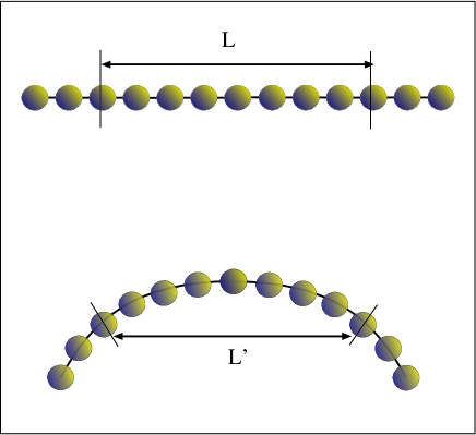
FIG. 1.: Schematic representation of buckling. In a buckled chain the effective separation between segments becomes smaller which lowers the free energy of the chain if the interactions between segments are attractive. This decrease in the free energy works against the increased bending energy thus leading to an instability.

FIG. 2.: Critical strength of the interaction potential, in terms of $V_{cr}~{}L^{2}$, as a function of the length of the rod, $L$, at different values of the screening parameter $r_{0}$ for the three models of attractive potentials: Finite potential well, Eq. (23), exponential potential, Eq. (26), and the general correlation potential, Eq. (35). The dependencies have been rescaled in such a way that at large $L$ they coincide.

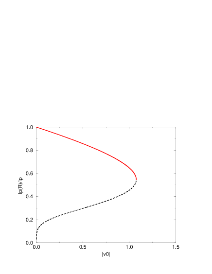
FIG. 3.: The solution of Eq. (69), the relation between the strength of segmental attraction and the change in apparent bending modulus, for $\kappa{\ell}_{p}=0.1$. Observe that ${\ell}_{p}^{(R)}/{\ell}_{p}$ depends linearly on $|v_{0}|$ for small values of $|v_{0}|$. There exists a $|v_{0c}|$ where there is no longer a physically acceptable solution for ${\ell}_{p}^{(R)}/{\ell}_{p}(|v_{0}|)$, implying a loss of stability of the coiled configuration of the polyelectrolyte chain. It is worth observing that $|v_{0c}|$ is not significantly larger than $k_{B}T$.

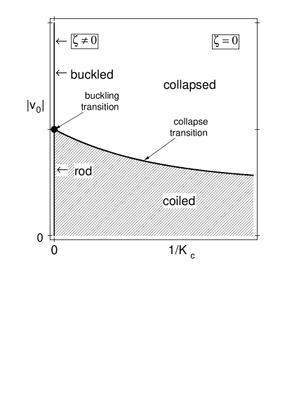
FIG. 4.: The phase diagram for a semi-flexible polymer whose bending rigidity is $K_{c}$, and whose monomers interact via an attractive potential of strength $|v_{0}|$. Buckling of a rod may take place for some $|v_{0}|$ when the bending rigidity is effectively infinite. Collapse of a random coil may take place for some $|v_{0}(K_{c})|$ when $K_{c}$ is finite.

REFERENCES

- [1] V. A. Bloomfield, DNA condensation, Curr. Op. Struc. Biol. 8, 334-341 (1996).
- [2] S. Strey, R. Podgornik, D.C. Rau and V.A. Parsegian, Curr. Op. Struc. Biol. (1998), in press.
- [3] R. Podgornik and V.A. Parsegian, Phys. Rev. Lett. 80, 1560 (1998) .
- [4] S. Leikin and A. Kornyshev, preprint (1998).
- [5] B.-Y. Ha and A. Liu, Phys. Rev. Lett. 79, 1289 (1997).
- [6] B.-Y. Ha and A. Liu, Phys. Rev. Lett. 81, 1011 (1998).
- [7] A.Yu.Grosberg and A.R.Khokhlov, Adv.Polym.Sci. 41, 53 (1981).
- [8] I.A. Nyrkova, N.P. Shusharina, and A. R. Khokhlov, Macromol.Theory Simul. 6, 965 (1997).
- [9] R. Golestanian, M. Kardar, T. B. Liverpool, cond-mat/9901293 (1999).
- [10] Stephen P. Timoshenko, J. Gere, Theory of Elastic Stability, 2nd Ed. (McGraw-Hill Book Company, New York,1969).
- [11] G. Manning, Cell Biophys. 7, 57 (1985).
- [12] T. Odijk, J. Chem. Phys. 108, 6923-6928 (1998).
- [13] I. Tobias, B.D. Coleman, W.K. Olson, J. Chem. Phys. 101, 10990-10996 (1994).
- [14] O. Spalla and L. Belloni, Phys. Rev. Lett. 74, 2515 (1995).
- [15] L.D. Landau and E.M. Lifshitz, Theory of Elasticity, Volume 7 of Course of Theoretical Physics, Third English Edition (Pergamon Press, Oxford, 1986).
- [16] R. P. Feynman and A.R. Hibbs, Quantum Mechanics and Path Integrals (McGraw-Hill Book Company, New York, 1965).
- [17] A. Erdelyi, Ed. Higher Transcendental Functions, Volume III (Mcgraw-Hill Book Company, Inc., New York, 1955).
- [18] M. Abramowith and I.A. Stegun, Handbook of Mathematical Functions (Dover, New York, 1965).
- [19] D.C. Khandekar and S.V. Lawande, Phys. Rep. 137, 115-229 (1986).
- [20] M. Grothaus, D.C. Khandekar, J.L. da Silva , L. Streit, J. Math. Phys. 38, 3278-3299 (1997).
- [21] H. Kleinert and A. Chervyakov, preprint physics/9/12048 (1997).
- [22] The 1/ expansion is similar to the 1/ expansion for spin systems. The 1/ expansion is discussed by S. K. Ma, Rev. Mod. Phys. 45 , 589 (1973); S. K. Ma,Modern Theory of Critical Phenomena (Addison-Wesley, New York, 1976); A. M. Polyakov, Gauge Fields and Strings (Harwood Academic Publishers, Churs, 1987). The 1/ is discussed by F. David, in Statistical Mechanics of Membranes and Interfaces, edited by D. Nelson, T. Piran and S. Weinberg (World Scientific, Singapore, 1989).
- [23] F. David and E. Guitter, Europhys. Lett. 3, 1169 (1987); Nucl. Phys. B295, 332 (1988).
- [24] P. Le Doussal, J. Phys. A: Math. Gen. 25, L469 (1992).
- [25] E. Guitter and J. Palmeri, Phys. Rev. A 45 , 734 (1992).
- [26] F. David and E. Guitter, Europhys. Lett. 5, 709 (1988); M. Paczuski and M. Kardar Phys. Rev. A 39 , 6086 (1989).
- [27] D. Thirumalai and B.-Y. Ha, in Theoretical and Mathematical Models in Polymer Research, edited by A. Grosberg (Academic Press, Boston,1998).
- [28] A. M. Polyakov, Gauge Fields and Strings (Harwood Academic Publishers, Churs, 1987).
- [29] E. Guitter, F. David, S. Leibler, and L. Peliti, Phys. Rev. Lett. 61 , 2949 (1988); E. Guitter, F. David, S. Leibler, and L. Peliti, J. Phys. France 50 , 1787 (1989).
- [30] The formalism developed here has the following pleasing feature. If we choose a Debye-Hückel interaction between monomers, and assume (), we determine an electrostactic contribution to the rigidity, in quantitative agreement with the celebrated results obtained by Odijk [31]; Skolnick & Fixman [32]; and Joanny & Barrat [33].
- [31] T. Odijk, J. Polym. Sci. 15, 477 (1977).
- [32] J. Skolnick and M. Fixman Macromolecules 10, 944 (1977).
- [33] J.-L. Barrat and J. F. Joanny Europhys. Lett. 24, 333 (1993).
- [34] A. Yu. Grosberg and A. Khokhlov, Statistical Physics of Macromolecules (AIP Press, New York, 1994).
- [35] I. Rouzina and V.A. Bloomfield, Biophys. J. 74, 3152 (1998).
- [36] P. L. Hansen and R. Podgornik, in preparation.