Structure-Property Correlations in Model Composite Materials

Abstract

We investigate the effective properties (conductivity, diffusivity and elastic moduli) of model random composite media derived from Gaussian random fields and overlapping hollow spheres. The morphologies generated in the models exhibit low percolation thresholds and give a realistic representation of the complex microstructure observed in many classes of composites. The statistical correlation functions of the models are derived and used to evaluate rigorous bounds on each property. Simulation of the effective conductivity is used to demonstrate the applicability of the bounds. The key morphological features which effect composite properties are discussed.

I Introduction

The prediction of effective properties of heterogeneous systems such as porous media and two phase composites is of considerable interest [3, 4, 5]. Understanding the inter-relationships between rock properties and their expression in geophysical and petrophysical data is necessary for enhanced characterisation of underground reservoirs. This understanding is crucial to the economics of oil and gas recovery, geothermal energy extraction and groundwater pollution abatement. Manufactured composites such as foamed solids [6] and polymer blends [7] often exhibit a complex microstructure. To optimize the properties of these systems it is necessary to understand how morphology influences effective properties. In general, the difficulty of accounting for microstructure has made exact prediction impossible in all but the simplest of cases.

On the other hand, considerable progress has been made in the derivation of rigorous bounds on a host of properties [3, 8]. For example, relatively accurate bounds have been derived for the elastic moduli and conductivity of isotropic two-phase composites [9, 10, 11, 12, 13]. To evaluate these bounds for a given system it is necessary to know the 3-point statistical correlation function [14]. Due to the difficulty of measuring this information [15, 16, 17], a number of model media have been proposed for which the functions can be explicitly evaluated. These include: cellular [18], particulate [3] and periodic [19] materials (eg. Figs. 1(a)&(b)). The principal problem with these models is that they employ over-simplified representations of the inclusion (or pore) structure observed in many natural and manufactured composite materials.

Recently we derived the properties of a model of amorphous materials [20] (e.g. Fig. 1(c)) based on level-cut Gaussian random fields [21] (GRF). Although the GRF model is applicable to many classes of non-particulate composite materials, it cannot account for materials which remain percolative at very low volume fractions.

Porous rocks [5, 22], polymer blends [7], solid foams [6] and membranes provide examples of systems where a single phase remains connected down to low volume fractions. The percolation threshold of a system is only one factor which determines its effective properties: The shape of the pores/inclusions should also be considered [23, 24, 25]. Polystyrene foam, an example of a highly-porous material, is shown in Fig. 2.

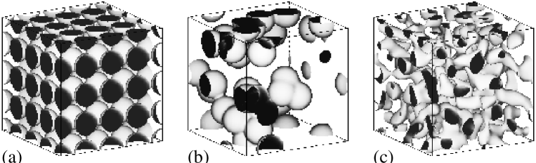
FIG. 1.: Models of composite microstructure. (a) Periodic models - regular array of spheres; (b) Particulate models - identical overlapping spheres (IOS) and; (c) Gaussian random field (GRF) models - single cut variant. None of the models can mimic the microstructure observed in percolative low volume fraction materials (e.g. polystyrene foam - Fig. 2).

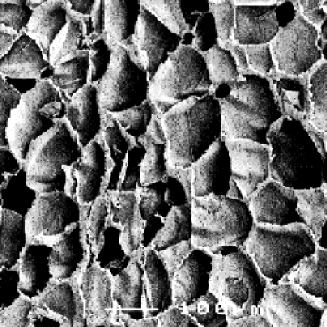
FIG. 2.: Morphology of polystyrene foam.

The complex solid phase has a ‘sheet-like’ character quite different to that found in cellular, particulate [3] and single level cut GRF [16, 20] models (Fig. 1). It is clear that current models of composite microstructure cannot account for the percolative and morphological characteristics observed in porous rocks, solid foams, membranes and polymer blends.

In this paper we describe models which do give a realistic representation of the microstructure observed in many classes of composite materials, and which remain percolative at very low volume fractions. Variational bounds and computer simulation are used to estimate the influence of morphology on diffusive-transport and elastic properties. The first model is an extension of the Gaussian random field (GRF) model considered in a previous paper [20]. In this case the interface between the composite phases is defined by two (rather than one) level cut of a GRF [21, 26, 27, 28]. The freedom in choosing the position of the cuts (for a given volume fraction), and the spectra of the model, allows a rich variety of morphologies to be modelled. By qualitatively comparing these morphologies to those observed in physical systems the models can be associated with classes of physical composites.

A second highly porous model can be obtained by generalizing the well-known IOS model [3] to include the case of arbitrarily thin hollow spheres. This model is applicable to a class of ceramics and foams fabricated from hollow spheres: a composite which possesses excellent uniformity and properties [29].

To study the properties of these media we evaluate bounds on the effective conductivity and elastic moduli. The key microstructure parameters ($\zeta_{1}$ & $\eta_{1}$) which occur in the derivation of the bounds [14] are tabulated along with illustrations of the model morphologies. In addition we use a finite difference scheme to directly simulate the effective conductivity. This allows us to comment on the applicability of the bounds, and on their use for predictive purposes.

The paper is organized as follows. In Section II we derive the 3-point correlation function for the 2-level cut Gaussian random field. In Section III analogous results are derived for the ‘identical overlapping spherical annuli’ (IOSA) or ‘hollow sphere’ model. In Sections IV and V the microstructure parameters are calculated, and computer simulations of the effective conductivity are compared with the resultant bounds. In section VI we discuss the influence of morphology on the transport and mechanical properties of composites.

II The 2-level cut GRF model

As in [20] we take $y({\mathbf{r}})$ as an isotropic Gaussian random field with a given field-field correlation function $\langle y({\mathbf{r}}_{i})y({\mathbf{r}}_{j})\rangle=g_{\mbox{$K$}}(r_{ij})$. Here $r_{ij}=|{\mathbf{r}}_{i}-{\mathbf{r}}_{j}|$ and for convenience we denote $g_{\mbox{$K$}}(r_{ij})$ by $g_{ij}$, or simply $g$ if no ambiguity arises. Following Berk [21] it is possible to define a composite medium with phase 1 the region in space where $\alpha\leq y({\mathbf{r}})\leq\beta$. The remaining region is phase 2. In the limit $\beta\to\infty$ the 1-level cut GRF considered in Refs. [20, 28] is recovered. The $n$-point correlation function is given by

$$p_{n}({\mathbf{r}}_{1},{\mathbf{r}}_{2},\dots,{\mathbf{r}}_{n})=\left\langle\prod_{i=1}^{n}\left[H(y_{i}-\alpha)-H(y_{i}-\beta)\right]\right\rangle,$$ (1)

where $H(y)$ is the Heaviside function and $y_{i}=y({\mathbf{r}}_{i})$.

The microstructure of the material is fully determined by specifying $\alpha$, $\beta$ and $g_{\mbox{$K$}}(r)$. The latter quantity is related to the spectral density of the field $\rho_{\mbox{$K$}}(k)$ by a clipped Fourier transform:

$$g_{\mbox{$K$}}(r)=\int_{0}^{K}4\pi k^{2}\rho_{\mbox{$K$}}(k)\frac{\sin kr}{kr}dk.$$ (2)

It was shown in [20] that few differences arise amongst the conductivity of the 1-level cut Gaussian random fields defined with differing spectra. Therefore we employ two model materials which showed the greatest variation in properties. In the notation of [20] these are Model I:

$$\rho(k) = P^{-1}\pi^{-2}\left((1-\nu^{2}+k^{2})^{2}+4\nu^{2}\right)^{-1}$$ (3)

$$\lim_{K\to\infty}g_{\mbox{$K$}}(r) = e^{-r}\frac{\sin\nu r}{\nu r},$$ (4)

where $P$ is a normalization constant chosen to ensure $g_{\mbox{$K$}}(0)=1$, and Model III:

$$\rho(k) = \frac{3}{4\pi(\mu^{3}-1)}[H(\mu)-H(1)]\;\;(\mu>1)$$ (5)

$$g(r) = \frac{3\left(\sin\mu r-\mu r\cos\mu r-\sin r+r\cos r\right)}{r^{3}(\mu^{3}-1)}.$$ (6)

No normalization constant is necessary in this model provided that $K\geq\mu$. In following sections we employ spectrum I ($\nu=0$, $K=\infty$), spectrum I ($\nu=0$, $K=8$) and spectrum III ($\mu=1.5$). In this paper the physical parameters $\nu$ and $\mu$ are not varied and will no longer be explicitly stated.

In the notation of Appendix A the 1-point correlation function (or volume fraction) is just

$$p=\Lambda_{1}(\alpha)-\Lambda_{1}(\beta)=\frac{1}{\sqrt{2\pi}}\int_{\alpha}^{\beta}e^{-\frac{1}{2}t^{2}}dt.$$ (7)

The 2-point correlation function for the 2-level cut Gaussian random field can be defined as

$$p_{2}=p^{2}+\Lambda_{2}(g,\alpha,\alpha)-2\Lambda_{2}(g,\alpha,\beta)+\Lambda_{2}(g,\beta,\beta)$$ (8)

where we have used the fact that $\Lambda_{2}(g,\alpha,\beta)=\Lambda_{2}(g,\beta,\alpha)$ and $p_{2}(g=0)=p^{2}$. Now using Eqn. (A9) leads to [27]

$$p_{2}(g)=p^{2}+\frac{1}{2\pi}\int_{0}^{g}\frac{dt}{\sqrt{1-t^{2}}}\times\left[\exp\left({-\frac{\alpha^{2}}{1+t}}\right)\right.$$ (9)

$$\left.-\exp\left({-\frac{1}{2}\frac{\alpha^{2}-2\alpha\beta t+\beta^{2}}{(1-t^{2})}}\right)+\exp\left({-\frac{\beta^{2}}{1+t}}\right)\right].$$ (10)

Similarly the 3-point correlation function is,

$$p_{3}=p^{3} + \Lambda_{3}({\mathbf{g}},\alpha,\alpha,\alpha)-\Lambda_{3}({\mathbf{g}},\alpha,\alpha,\beta)-\Lambda_{3}({\mathbf{g}},\alpha,\beta,\alpha)$$ (11)

$$- \Lambda_{3}({\mathbf{g}},\beta,\alpha,\alpha)+\Lambda_{3}({\mathbf{g}},\alpha,\beta,\beta)+\Lambda_{3}({\mathbf{g}},\beta,\alpha,\beta)$$ (12)

$$+ \Lambda_{3}({\mathbf{g}},\beta,\beta,\alpha)-\Lambda_{3}({\mathbf{g}},\beta,\beta,\beta)$$ (13)

where $\Lambda_{3}$ is given in Eq. A22 and ${\mathbf{g}}=(g_{12},g_{13},g_{23})$. We could find no symmetries in these terms to allow analytical or computational simplification of the results.

For our purposes it is necessary to choose $\alpha$ and $\beta$ for a given value of the volume fraction $p$. There are many ways that this can be done. An obvious method is to require that an equivalent fraction of phase 1 lies on either side of a particular level cut $y({\mathbf{r}})=\gamma$. We classify these ‘symmetric’ models by the parameter

$$s=\frac{1}{\sqrt{2\pi}}\int_{\gamma}^{\infty}e^{-\frac{1}{2}t^{2}}dt$$ (14)

so that $s\in[0,1]$. For a given volume fraction $p$, $\alpha$ and $\beta$ are defined through the relations

$$\frac{p}{2}=\frac{1}{\sqrt{2\pi}}\int_{\alpha}^{\gamma}e^{-\frac{1}{2}t^{2}}dt=\frac{1}{\sqrt{2\pi}}\int_{\gamma}^{\beta}e^{-\frac{1}{2}t^{2}}dt$$ (15)

Materials defined in this manner are denoted by, for example, III(s=.5). This indicates that the spectrum of model III is employed and that $s=0.5$ (corresponding to the case $\alpha=-\beta$). For comparison with the 1-level cut case discussed in [20] it is also useful to define a 2-level cut GRF which reduces to the former model in a particular limit. This is done by fixing $\beta$ and varying $\alpha$ such that a given volume fraction is achieved. These ‘base’-level models are specified by the value

$$b=\frac{1}{\sqrt{2\pi}}\int_{\beta}^{\infty}e^{-\frac{1}{2}t^{2}}dt$$ (16)

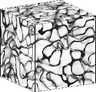
FIG. 3.: The interface of the media III(s=.5) at a volume fraction of $p=0.2$. The dark region is given by $-0.253<y({\bf r})<0.253$. Note the highly connected structures.

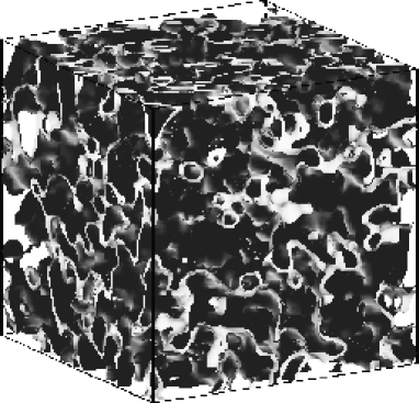
FIG. 4.: The interface of the media I(s=.5) with a pore volume fraction of $p=0.2$. The light region corresponds to $-0.253<y({\bf r})<0.253$.

where $b\in[0,1]$. Since $\beta$ is fixed, $\alpha$ is calculated using Eqn. (7). In terms of nomenclature used to describe the spectra previously these models are denoted, for example, as III(b=.3) or I(b=0) (ie. $\beta=\infty$). The latter case corresponds to the 1-level cut field.

Depending on the spectra employed and the choice of $\alpha$ and $\beta$ the 2-cut GRF scheme can model a wide range of morphologies observed in physical composites. The morphology of 1-cut fields is characterized by a random array of irregular inclusions interconnected by narrower necks [20] similar to a ‘node/bond’ geometry (see

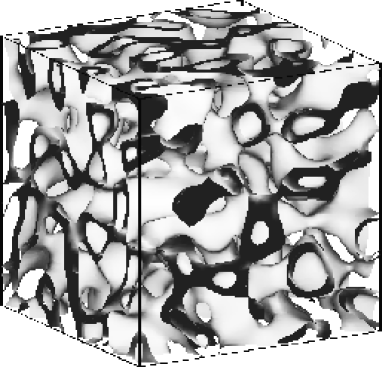
FIG. 5.: The interface of the media III(s=.2) at a volume fraction of $p=0.2$. The dark region is given by $-1.28<y({\bf r})<-0.253$.

Fig. 1(c)). This type of pore/inclusion shape has been observed in a range of materials including alloys [30] and sedimentary rocks [23]. Taking $\beta\!\!=\!\!-\alpha$ in the 2-cut model $(s=0.5)$ leads to ‘sheet-like’ structures (see Figs. 3 & 4) with differing degrees of roughness. The smooth-sheet like structures of model III(s=.5) (Fig. 3) are similar to the pores observed in dolomitic limestone [31], and the connected matrix in solid foams [32] (see Fig. 2) and polymer blends [33]. The rough ‘sheet-like’ morphology evident in model I(s=.5) ($K=8$) (Fig. 4) is similar to the rough porous structures observed in pore-cast studies of sandstones [16, 23]. Note that certain classes of sandstone have been shown to have a fractal pore surface with $D_{s}\approx 2.5$ [34]. This can be modelled by taking $K\to\infty$ in spectrum I (Appx. B). Qualitatively different microstructures can be obtained in the 2-cut scheme if $\beta\neq\alpha$. For example, the morphology of Model III(s=.2) (Fig. 5) has both a node/bond and sheet-like quality.

III Overlapping hollow spheres

A second low porosity model can be defined by generalizing the ‘Identical Overlapping Sphere’ (IOS) model to the case of overlapping annuli (IOSA). For this model the probability that $n$ points ${\mathbf{r}}_{i}$ chosen at random will fall in the void phase (ie. outside the hollow spheres) is just

$$q_{n}=\exp[-\rho V\!a^{(n)}_{U}({\mathbf{r}}_{1},\dots,{\mathbf{r}}_{n})].$$ (17)

Here $V\!a^{(n)}_{U}$ is the union volume of $n$ spherical annuli with centers at ${\mathbf{r}}_{i}$, and $\rho$ is the number density of the annuli.

To see this consider a large region of the composite material of volume $V$ which contains $N=\rho V$ randomly positioned (i.e. uncorrelated) spherical annuli. Now consider $q_{n}$ defined above. If, and only if, the center of an annulus is located within the volume $V\!a^{(n)}_{U}$, then one (or more) of the $n$ points will lie in the solid phase. Since each annulus is uniformly distributed the probability that its center will not fall in the volume $V\!a^{(n)}_{U}$ is $(1-V\!a^{(n)}_{U}/V)$. Now there are $N$ such uncorrelated spheres so

$$q_{n}=\lim_{N\to\infty}\left({1-\frac{\rho V\!a^{(n)}_{U}}{N}}\right)^{N}=\exp\left({-\rho V\!a^{(n)}_{U}}\right)$$ (18)

where $V$, and hence $N$, has been taken to be infinitely large. This argument (for the spherical case) is due to W. F. Brown [35, 36]. By definition $q_{n}$ is just the $n$-point void-void correlation function. To distinguish the correlation functions associated with the void and solid we refer to above model as the inverse IOSA model (as the correlation function corresponds to the phase outside the annuli). The correlation functions for the IOSA model ($p_{n}$) are then just linear combinations of $q_{n}$, $q_{n-1}$ etc. For example, $p_{1}=1-q_{1}$ and $p_{2}(r_{12})=1-2q+q_{2}(r_{12}).$

Suppose the inner and outer radii of the annuli are $\mu$ and $\nu$, then the union volume of a single annulus is $V\!a=V\!a^{(1)}_{U}=4\pi(\nu^{3}-\mu^{3})/3$. The number density of the annuli is related to the volume fraction of void ($q$) by the formula $\rho=-{\log q}/{V\!a}$. The higher order union volumes are derived in terms of the intersection volumes of spheres of different radii. For the union volume of two annuli a distance $d$ apart we have

$$V\!a^{(2)}_{U}(d)=2V\!a-V\!a^{(2)}_{I}(d)$$ (19)

where $V\!a^{(2)}_{I}(d)$ is the intersection volume of 2 annuli. This function is given by

$$V\!a^{(2)}_{I}(d)=V^{(2)}_{I\nu\nu}(d)+V^{(2)}_{I\mu\mu}(d)-2V^{(2)}_{I\mu\nu}(d)$$ (20)

with $V^{(2)}_{Ixy}(d)$ the intersection volume of two spheres of radii $x$ and $y$ (see Appendix C). The union volume of the three annuli distances $a$, $b$ & $c$ apart is

$$V\!a^{(3)}_{U}(a,b,c) = 3V\!a-V\!a^{(2)}_{I}(a)-V\!a^{(2)}_{I}(b)-V\!a^{(2)}_{I}(c)$$ (22)

$$+V\!a^{(3)}_{I}(a,b,c),$$

where the intersection volume of three annuli ($V\!a^{(3)}_{I}$) is

$$V\!a^{(3)}_{I} = V^{(3)}_{I\nu\nu\nu}-V^{(3)}_{I\mu\mu\mu}-V^{(3)}_{I\mu\nu\nu}-V^{(3)}_{I\nu\mu\nu}-V^{(3)}_{I\nu\nu\mu}$$ (24)

$$+V^{(3)}_{I\mu\mu\nu}+V^{(3)}_{I\mu\nu\mu}+V^{(3)}_{I\nu\mu\mu}.$$

Here the function $V^{(3)}_{Ixyz}(a,b,c)$ is the intersection volume of three spheres of radii $x$, $y$ and $z$ with $a$ the distance between the spheres of radii $y\;\&\;z$, $b$ the distance between the spheres of radii $x\;\&\;z$ and $c$ the distance between the spheres $x\;\&\;y$ (see Appendix C).

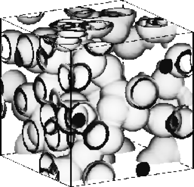
FIG. 6.: The interface of the IOSA model ($r_{0}=0.8$, $r_{1}=1.0$) at a volume fraction of $p=0.2$.

As in the 2-level cut GRF model there are two obvious ways of choosing the internal ($r_{0}=\mu$) and external ($r_{1}=\nu$) radii for a given volume fraction. In the first the internal radii of the spheres is held fixed and the number density of spheres is increased to achieve a given volume fraction. This model morphology corresponds to manufactured materials comprised of sintered similarly sized hollow spheres [29]. A plot of the interface for the IOSA model is given for the case $r_{0}=0.8$ and $p=0.2$ in Fig. 6. Using results [3, 37, 38, 39] developed for overlapping solid spheres (ie. IOS) it is possible to incorporate a distribution of sphere sizes in the hollow sphere model. However, polydispersity effects have been shown to be quite small [40]. In the second model the number density of spheres is held fixed (so that the maximum volume fraction achievable is $p_{max}$) and the internal radii is varied to achieve a given volume fraction.

The percolation thresholds of each phase of the IOSA model $p_{c}^{a}$ (solid) & $q_{c}^{a}$ (void), can be easily derived from a knowledge of the threshold values of the standard IOS model: $p_{c}^{s}\approx 0.3$ [41] and $q_{c}^{s}\approx 0.03$ [42]. For the variable density model ($r_{0}$ fixed) the percolation thresholds are $p_{c}^{a}=1-(1-p_{c}^{s})^{1-(r_{0}/r_{1})^{3}}$ and $q_{c}^{a}=(q_{c}^{s})^{1-(r_{0}/r_{1})^{3}}$ (so $p_{c}^{a}\to 0$ & $q_{c}^{a}\to 1$ as $r_{0}\to r_{1}$). For the fixed density model the IOSA solid phase is percolative if $p_{max}\geq p_{c}^{s}$ and the void phase is percolative if $q_{min}=1-p_{max}\geq q_{c}^{s}$.

IV Microstructure parameters

Bounds have been calculated on the conductivity [9, 12] and the bulk [10] and shear [11, 13] moduli of composite materials (reviewed in Ref. [3]). These can be expressed [14] in terms of the volume fractions and properties of each of the phases and two microstructure parameters:

$$\zeta_{1} = \frac{9}{2pq}\int_{0}^{\infty}\!\!\frac{dr}{r}\int_{0}^{\infty}\!\!\frac{ds}{s}\int_{-1}^{1}\!\!duP_{2}(u)f(r,s,t)$$ (25)

$$\eta_{1} = \frac{5\zeta_{1}}{21}+\frac{150}{7pq}\int_{0}^{\infty}\!\!\frac{dr}{r}\int_{0}^{\infty}\!\!\frac{ds}{s}\int_{-1}^{1}\!\!duP_{4}(u)f(r,s,t)$$ (26)

where $f(r,s,t)=p_{3}(r,s,t)-p_{2}(r)p_{2}(s)/p$, $t^{2}=r^{2}+s^{2}-2rsu$ and $P_{n}(u)$ denotes the Legendre polynomial of order $n$. As we argued in Ref. [20] it only appears necessary to know broad microstructural information about a general composite to successfully apply the bounds. This conclusion arose from the observation that the bounds are relatively insensitive to small variations in the microstructure parameters. Furthermore we found that the parameters $\zeta_{1}$ and $\eta_{1}$ are insensitive to fine microstructural details within a class of composites (e.g. the overlapping sphere class, or the 1-level cut GRF class). An example of this insensitivity is also seen when polydispersity effects of particulate models are considered [40]. In light of these facts the parameters calculated from models may well have application to physical composites for which precise microstructural information is unavailable.

In Fig. 7 we provide a graphical summary of the wide range of isotropic composites for which $p_{3}$ (and hence the microstructure parameters) can been exactly calculated. It is clear that the 2-cut GRF and overlapping hollow sphere model considerably expand the classes of materials to which the bounds can be applied.

We now report calculations of the microstructure parameters for a variety of 2-level cut GRF and IOSA models. Our method of calculating $\zeta_{1}$ (and $\eta_{1}$) has been discussed previously [20]. In addition we employ an adaptive integration algorithm [43] to compensate for the fact that the sub-integrand $\int_{-1}^{1}P_{n}(u)f(r,s,t)du$ varies rapidly in the region $r\approx 0$ and involves a considerable number of function evaluations. The error in the results is less than 1%. To model as wide a range of materials as possible three qualitatively different spectra are used in the level-cut GRF scheme; models I ($K=\infty$), I ($K=8$) and III ($\mu=1.5$). These spectra lead to surface-fractal, rough and smooth interfaces respectively.

As we are primarily interested in low volume fraction porous or solid media the microstructure parameters we report are in the range $0.0<p\leq 0.4$. The results for $\zeta_{1}$ and $\eta_{1}$ are given in Tables I & II and selected results are plotted in Figs. 8 & 9. The results for the two variants of the IOSA model are given in Table III and plotted along side the results for the 2-cut GRF models in Figs. 8 & 9. Due to the simple geometry of the IOSA model it is possible to calculate $\sigma_{e}$ to order $p$ (see Appendix D). This result can then be used to show $\zeta_{1}|_{p=0}=(r_{0}/r_{1})^{3}$ (represented by symbols in Fig. 8) in agreement with our numerical calculations of $\zeta_{1}$.

To compare the properties of different media we plot (Fig. 10) the upper bound on the conductivity for one member of each class of composite: 2-cut GRFs, hollow spheres, IOS-voids [36] (or swiss-cheese), 1-cut GRFs [20] and IOS [36] (or solid spheres).

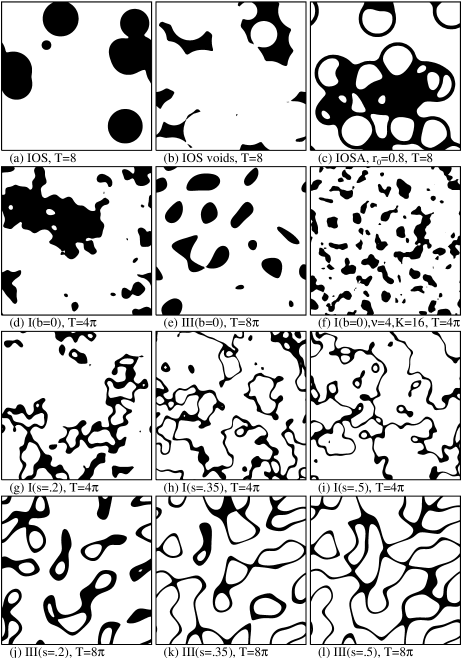
FIG. 7.: A variety of microstructures (volume fraction 20%) for which the third order statistics are known exactly: (a)-(c) IOS and IOSA models ($r_{1}=1$); (d)-(f) 1-level cut GRF’s; (g)-(l) 2-level cut GRF’s. Except where noted Model I has $K=8$ & $\nu=0$ and Model III $\mu=1.5$.

TABLE I.: The microstructure parameter $\zeta_{1}$ for a range of materials generated from the symmetric GRF model.

Mod.	I, $K=\infty$			I, $K=8$			III
s	.20	.35	.50	.20	.35	.50	.20	.35	.50
p	$\zeta_{1}$
.050	.401	.401	.402	.706	.773	.786	.785	.872	.892
.075	.402	.408	.409	.641	.719	.739	.733	.845	.873
.100	.405	.413	.415	.597	.684	.706	.691	.824	.858
.125	.410	.422	.425	.563	.655	.677	.655	.807	.845
.150	.417	.428	.431	.536	.633	.656	.625	.791	.828
.200	.425	.443	.449	.500	.601	.628	.574	.769	.819
.250	.435	.459	.464	.478	.583	.611	.532	.753	.811
.300	.443	.475	.481	.464	.575	.605	.495	.741	.808
.350	.451	.491	.497	.455	.572	.603	.456	.734	.807
.400	.456	.506	.515	.444	.574	.607	.411	.728	.810

TABLE II.: The elasticity microstructure parameter $\eta_{1}$ for a range of materials generated using the symmetric GRF model.

Mod.	I, $K=\infty$		I, $K=8$		III
s	.20	.50	.20	.50	.20	.50
p	$\eta_{1}$
.050	.355	.351	.523	.613	.609	.754
.075	.358	.362	.463	.548	.543	.705
.100	.362	.369	.430	.516	.500	.672
.125	.370	.377	.416	.493	.471	.648
.150	.373	.388	.407	.480	.449	.608
.200	.394	.402	.404	.473	.426	.621
.250	.410	.430	.410	.478	.414	.609
.300	.426	.451	.420	.492	.408	.615
.350	.438	.474	.430	.510	.406	.627
.400	.442	.495	.431	.533	.396	.643

TABLE III.: The microstructure parameters for different versions of the IOSA model. For the case $r_{0}=0$ the results are just those of the standard IOS model (see Ref. [3]).

Mod.	$r_{0}=0.5$		$r_{0}=0.9$		$p_{max}=0.9$		$p_{max}=0.7$
p	$\zeta_{1}$	$\eta_{1}$	$\zeta_{1}$	$\eta_{1}$	$\zeta_{1}$	$\eta_{1}$	$\zeta_{1}$	$\eta_{1}$
.05	.152	.119	.737	.468	.974	.936	.955	.888
.10	.179	.153	.744	.490	.948	.880	.911	.788
.15	.207	.187	.752	.512	.924	.827	.870	.707
.20	.234	.221	.759	.533	.900	.780	.829	.640
.25	.262	.254	.766	.554	.877	.746	.791	.590
.30	.289	.288	.772	.576	.856	.710	.754	.551
.35	.317	.322	.778	.596	.835	.683	.718	.524
.40	.345	.356	.784	.616	.815	.662	.683	.508
.50	.402	.424	.794	.656	.776	.638	.614	.502
.60	.459	.492	.801	.697	.741	.631	.539	.520
.70	.517	.560	.805	.733	.706	.643	.414	.511
.80	.578	.630	.804	.771	.666	.668
.90	.643	.705	.792	.804	.558	.658

We have also evaluated bounds on the shear, bulk and Young’s moduli of the models. In Ref. [32] we showed that the upper bound on Young’s modulus was in good agreement with experimental measurements for foamed solids. Model III(s=.5) provides a good model of polystyrene foam (compare Figs. 2 & 3), and the IOSA model accurately mimics the microstructure and properties of sintered hollow glass spheres. In Fig. 11 the upper bound on the shear modulus is shown for each class of composite considered above: the microstructure clearly has a strong influence on elastic properties. The bulk and Young’s moduli show similar behaviour.

V Simulations of $\sigma_{e}$

In addition to bounding the properties of composite media and providing qualitative information on these properties, it has been observed that the bounds also have reasonable predictive power [3]. To test the predictive utility of the bounds and provide a direct

FIG. 8.: The microstructure parameter $\zeta_{1}$ for selected models. The IOS model and model III(b=0) are included to show the behaviour of $\zeta_{1}$ for different classes of composites (see Fig. 7). The solid symbols represent analytic calculations of $\zeta_{1}|_{p=0}$ for the IOSA model.

FIG. 9.: The elasticity microstructure parameter $\eta_{1}$ for selected models. The IOS model and model III(b=0) are included to show the behaviour of $\eta_{1}$ for different classes of composites (see Fig. 7).

comparison between microstructure and properties we use a finite-difference method to explicitly calculate the conductivity of several 2-cut GRF’s.

The effective conductivity $\sigma_{e}$ of a composite is defined as the ratio of the current density to the applied potential. We take $T$ as the scale of the sample and $M^{3}$ as the number of nodes (so the spatial resolution scale is $\Delta x=T/M$). The generation of random fields and the method for determining $\sigma_{e}$ were described in Ref. [20] for the case of 1-cut fields. A number of additional difficulties are encountered in the simulations of $\sigma_{e}$ for the 2-level cut GRF’s. The major problems are; (i) discretisation effects which occur when the discretisation length scale $\Delta x$ is insufficient to resolve the thin sheet-like structures which arise (e.g. Fig. 3) and (ii) finite-scale effects which arise if $T$ is not large enough to represent an ‘infinite’ medium. In practice $T$ should be several times the

FIG. 10.: The 3-point upper bound [9] on the effective conductivity (contrast 1:0) of five different classes of microstructure. The data for the IOS and 1-cut GRF models are from Refs. [36, 20].

FIG. 11.: The 3-point upper bound [13] on the effective shear modulus (contrast 1:0) of five different classes of microstructure. The data for the IOS and 1-cut GRF models are from Refs. [36, 20].

correlation length of the microstructure (approx. unity). Discretisation effects can be reduced by increasing $M$ or decreasing $T$ (to increase the width of the sheets relative to $\Delta x$). However our computational requirements dictate $M\leq 128$ and decreasing $T$ leads to noisy results. Thus $T$ must be chosen to minimize each of these competing errors. By performing several numerical tests [43] a reasonable value of $T$ was determined to ensure that simulations of $\sigma_{e}$ are accurate. As the sheets become

FIG. 12.: The simulation data and bounds for three different 2-level cut GRF models at contrast $\sigma_{1,2}=10,1$. The thick solid line corresponds to the bounds for the 1-level cut model III(b=0). The bounds are clearly seen to differentiate the different classes of media at low $p$.

TABLE IV.: The effective conductivity of several 2-level cut GRF’s for the case $\sigma_{1,2}=10,1$.

	III(s=.2)			III(s=.5)			I(s=.5)
p	$T/\pi$	$\sigma_{e}$	Err.	$T/\pi$	$\sigma_{e}$	Err.	$T/\pi$	$\sigma_{e}$	Err.
0.05	4	1.28	.01	2	1.32	.02	2	1.27	.00
0.10	4	1.51	.02	2	1.64	.03	2	1.53	.02
0.15	4	1.76	.04	2	1.96	.05	2	1.77	.02
0.20	4	2.02	.06	4	2.30	.07	2	2.05	.01
0.25	8	2.32	.03	4	2.58	.10	4	2.35	.01
0.30	8	2.61	.04	4	2.94	.12	4	2.67	.01
0.35	8	2.93	.03	4	3.30	.13	4	3.02	.01
0.40	8	3.25	.05	4	3.70	.13	4	3.40	.02

FIG. 13.: The simulation data and bounds for three different 2-level cut GRF models with conductivity $\sigma_{1,2}=50,1$.

TABLE V.: The effective conductivity of several 2-level cut GRF’s for the case $\sigma_{1,2}=50,1$.

	III(s=.2)			III(s=.5)			I(s=.5)
p	$T/\pi$	$\sigma_{e}$	Err.	$T/\pi$	$\sigma_{e}$	Err.	$T/\pi$	$\sigma_{e}$	Err.
0.05	4	2.3	0.2	2	2.6	0.2	1	2.1	0.1
0.10	4	3.4	0.4	2	4.1	0.4	1	3.3	0.1
0.15	8	4.1	0.1	2	5.7	0.5	1	4.2	0.1
0.20	8	5.1	0.2	2	7.4	0.7	1	5.4	0.1
0.25	8	6.4	0.2	4	9.3	0.2	2	7.0	0.1
0.30	8	7.8	0.2	4	11.2	0.3	2	8.6	0.1
0.35	8	9.3	0.3	4	13.2	0.3	2	10.4	0.2
0.40	8	10.9	0.4	4	15.3	0.3	2	12.3	0.2

 

thinner (ie. $p$ decreases) it was found that smaller values of $T$ are necessary to eliminate finite-scale effects. This can be explained in terms of the faster decay of the correlations between the components of phase 1.

We choose to study the effective conductivity of models III(s=.5), I(s=.5) ($K=8$) and III(s=.2). The former models provide examples of smooth and rough ‘sheet-like’ pores. The latter model (III(s=.2)) has a morphology comprised of inclusions with both a sheet- and node/bond-like quality. The conductivity contrasts employed occur in physical composites and have been studied previously, allowing comparisons to be made. In each of the cases we report results averaged over five samples for a range of volume fractions $0.05\leq p\leq 0.4$. In all cases the simulational data lie between the bounds.

First we consider the conductivity contrast $\sigma_{1,2}=10,1$. The results are tabulated in Table IV, and plotted in Fig. 12 along with the bounds for each model, Here, and in subsequent calculations, the lower bound of Beran [9] and the upper bound of Milton [12] (see Ref. [20]) are employed. The data for model III(s=.5) practically lies along the relevant upper bound. In contrast the effective conductivity of models III(s=.2) and I(s=.5) fall between the bounds, however the upper bound still provides a reasonable estimate of $\sigma_{e}$ in each case. For purposes of comparison the bounds for the 1-level cut GRF model III(b=0) are included in Fig. 12. At low $p$ the bounds clearly differentiate between the different classes of media. It is clear that the model III(s=.5) is a significantly more efficient conductor than models III(s=.2) or I(s=.5) and those defined using a 1-level cut GRF in [20].

The simulation data for the contrast $\sigma_{1,2}=50,1$ is reported in Table V and plotted in Fig. 13. Qualitatively the results are the same as those discussed in relation to the case $\sigma_{1,2}=10,1$. Note that the upper bound is again a good estimate for model III(s=.5); less so for models

FIG. 14.: Simulation data and bounds for conductivity contrast $\sigma_{1,2}=1,0$. The models and contrast are relevant to solid-foams [32] and porous rocks [49].

TABLE VI.: The effective conductivity of several 2-level cut GRF’s for the case $\sigma_{1,2}=1,0$.

	III(s=.2)			III(s=.5)			I(s=.5)
p	$T\!/\pi$	$\sigma_{e}$	Err.	$T\!/\pi$	$\sigma_{e}$	Err.	$T\!/\pi$	$\sigma_{e}$	Err.
.05	4	.018	.002	2	.034	.003	2	.011	.003
.10	4	.030	.004	2	.061	.003	2	.044	.005
.15	4	.050	.005	2	.095	.003	2	.058	.007
.20	4	.073	.007	4	.130	.004	2	.078	.009
.25	8	.094	.004	4	.165	.005	4	.111	.004
.30	8	.121	.003	4	.204	.005	4	.141	.004
.35	8	.154	.003	4	.245	.006	4	.177	.007
.40	8	.190	.002	4	.287	.007	4	.219	.006

FIG. 15.: Simulations of $\sigma_{e}$ and the bounds for $\sigma_{1,2}=0,1$. This contrast is relevant to modeling transport in membranes.

TABLE VII.: The effective conductivity of several 2-level cut GRF’s for the case $\sigma_{1,2}=0,1$.

	III(s=.2)			III(s=.5)
p	$T/\pi$	$\sigma_{e}$	Err.	$T/\pi$	$\sigma_{e}$	Err.
0.10	4	0.66	.02	2	0.55	.05
0.15	4	0.62	.02	2	0.49	.06
0.20	4	0.58	.02	2	0.43	.07
0.25	8	0.53	.01	4	0.34	.05
0.30	8	0.50	.01	4	0.29	.05
0.35	8	0.47	.01	4	0.24	.04
0.40	8	0.44	.01	4	0.20	.03

 

III(s=.2) and I(s=.5).

In porous rocks and solid foams the conductivity of the medium surrounding the conducting pathways has negligible (or zero) conductivity. To model such systems the contrast $\sigma_{1,2}=1,0$ is used. The data and computational parameters used in the simulations are reported in Table VI. Each material is seen to be conductive at the lowest volume fraction considered $p=0.05$. Discretisation effects prohibit accurate simulations of $\sigma_{e}$ at lower volume fractions. The simulation data and the upper bounds are plotted in Fig. 14. Even in this large contrast situation the upper bound for model III(s=.5) agrees with the data.

To consider the case of diffusive transport in membranes, we assume that the membrane has negligible diffusivity with respect to the surrounding fluid. Therefore the contrast $\sigma_{1,2}=0,1$ is employed. For this system large discretisation effects prohibit the consideration of model I(s=.5) and membrane/pore volume fractions of less than $p=0.10$. The data is presented in Table VII and Fig. 15. Note that the presence of a membrane occupying 10%-20% of the total volume reduces the diffusivity by a factor of two. This is due to the tortuous pathways through which the diffusing species must migrate. In contrast to three cases considered above the upper bound does not provide a good estimate of $\sigma_{e}$ for model III(s=.5).

VI Effect of microstructure on properties

The precise role of microstructure in determining the macroscopic properties of composite media has been the subject of many studies. A number of simple models of pore-shape have proposed to determine, for example, the effect of pore-size distribution [22], pore roughness [44] and pore geometry [23] on transport in porous rocks. Simple micro-mechanical models [45] have also been studied to ascertain, for example, the effect of inclusion shape [46] and cell structure [6, 47] on the mechanical properties of composites. In this section we investigate

TABLE VIII.: Qualitative comparison of microstructure and macroscopic properties. We consider the contrast 1:0 at a representative volume fraction $p=0.2$. $\sigma_{u}$, $\kappa_{u}$, and $\mu_{u}$ are upper bounds on the effective conductivity [9], bulk [10] and shear modulus [13] respectively.

Model	Microstructure	$p_{c}$	$\sigma_{e}$	$\zeta_{1}$	$\eta_{1}$	$\sigma_{u}$	$\kappa_{u}$	$\mu_{u}$
III(s=.5)	smooth, sheet-like	0	0.130	.819	.621	0.134	0.115	0.094
I(s=.5) $K=8$	rough, sheet-like	0	0.078	.628	.473	0.122	0.102	0.081
III(s=.2)	smooth, node/bond/sheet-like	0	0.073	.574	.426	0.118	0.098	0.077
I(s=.5) $K=\infty$	very rough, sheet-like	0	-	.449	.402	0.106	0.086	0.068
I(b=0)a$K=\infty$	very rough, node/bond-like	-	-	.366	.333	0.096	0.076	0.060
I(b=0)a$K=8$	rough, node/bond-like	.07	0.027	.326	.291	0.090	0.071	0.054
III(b=0)a	smooth, node/bond-like	.13	0.026	.237	.197	0.074	0.057	0.042
IOSA ($r_{0}=0.9$)	hollow spheres	.09	-	.759	.533	0.131	0.117	0.090
IOS-voids	swiss-cheese	.03b	0.076c	.518d	.416d	0.113	0.093	0.073
IOS	spheres	.30e	0	.113d	.148d	0.044	0.032	0.026

how morphology influences the properties of realistic model composites.

To simplify the discussion we summarize relevant data for a variety of GRF and particulate microstructure models in Table VIII. We consider systems of 1:0 contrast at $p=0.2$. This case corresponds to a conducting (mechanically strong) matrix in an insulating (weak) medium (e.g. foamed solids [32]). This contrast also corresponds to low porosity conducting pores in an insulating medium (e.g. porous rocks). To gauge the effect of microstructure on material properties we assume that the upper bound on each property provides an estimate of its actual value. A comparison of $\sigma_{u}$ and $\sigma_{e}$ (where available) shows that this is generally true [48]. Note, however, that if the difference between $\sigma_{u}$ for each of the models is small (e.g. IOS-voids and model III(s=.2) and examples in Ref. [20]) such an assumption cannot be made ($\sigma_{u}^{a}>\sigma_{u}^{b}$ but $\sigma_{e}^{a}<\sigma_{e}^{b}$).

At a 1:0 contrast the effective properties only differ from zero if the composite is macroscopically connected (i.e. percolative). At $p=0.2$ this condition is satisfied for all but one of the media (conducting spheres in an insulating medium). Above this threshold the magnitude of the macroscopic properties is then governed by the shape of the inclusions. It is clear from the table that sheet-like structures provide higher conductivity and mechanical strength than those with a node/bond-like character. To elucidate the role of inclusion shape we derive approximate expressions for the effective conductivity of periodic media with unit cells of each type in Appendix E. For small volume fractions ($p\ll 1$) the node/bond model has $\sigma_{e}\simeq p^{2}\sigma_{1}$ and the sheet-like model has $\sigma_{e}\simeq\frac{2}{3}p\sigma_{1}$ in qualitative agreement with the data. Interestingly the periodic sheet model provides a surprisingly good estimate of $\sigma_{e}=\frac{2}{3}0.2=0.133$ for model III(s=.5) ($\sigma_{e}=0.130$).

From the table it also evident that interfacial roughness plays an important role in determining properties. Consider the 2-cut fields I(s=.5) and III(s=.5). In Figs. 7(i) and 7(l) it is clear that both models contain sheet-like pores. The differences are then due to the interfacial roughness. This is confirmed by comparing the relative values of $\sigma_{u}$ for model I in the cases $K=8$ (smooth on scales below $\lambda_{min}=2\pi/8$) and $K=\infty$ (rough on all scales) - see Appx. B. The effect of increasing $K$ from 8 to 32 on the morphology of model I(s=.5) can be seen by comparing Fig. 7(i) & Fig. 16(a). In the rough model the sheet-like pores are thinner and a large proportion of pore space is distributed in protrusions. As these protrusions contribute little to the overall conductance (or strength), this significantly reduces both conductivity and strength. This also explains why Model III is more conductive (stronger) than Model I. The much smaller effect of roughness on morphology of 1-level cut fields can be seen by comparing Fig. 7(d) & Fig. 16(b): the basic inclusion shape is less affected than in the 2-cut case.

Now consider the data for the spherical particulate media in Table VIII. The hollow sphere model appears to be more conductive, or stronger, than the IOS-voids (swiss-cheese) model. This is due to the fact that the former model has an approximately sheet-like character (Fig. 6) in contrast to the node/bond-like structures [4] apparent in the inverse IOS model. The IOS model at $p=0.2$ does not have a sufficient density of spheres to provide a percolative pathway.

VII Conclusion

In this paper we have derived the 3-point statistical correlation functions for two models of random composite media. The results were applied in the evaluation of bounds on the effective conductivity and elastic moduli of each model. In addition the ‘exact’ effective conductivity was estimated for the 2-level cut GRF model by direct simulation. The models are applicable to physical composites which remain percolative at very low volume fractions $p_{c}<1\%$. These include solid foams, porous rocks, membranes and sintered hollow glass spheres. In contrast, previously employed models of microstructure have percolation thresholds of order 10%.

Microstructure was demonstrated to have a strong influence on the effective properties of composites. The relative variations amongst the 2-level cut, IOSA and 1-level cut models were attributed to three morphological factors; pore-shape, interfacial roughness and the percolation threshold of the material. Materials with sheet-like inclusions were shown to have a significantly greater conductivity/strength than materials with node/bond-like inclusions. By comparing the microstructure parameters of similar composites with fractally rough and relatively smooth inclusions we found that interfacial roughness decreased composite conductivity/strength. The observation was confirmed by directly comparing simulated values of $\sigma_{e}$ for Model I(s=.5) (sheet-like and rough) and Model III(s=.5) (sheet-like and smooth). The behaviour was physically attributed to the fact that the protrusions of rough interfaces contribute little to effective properties.

The models discussed here considerably expand the range of systems to which bounds can be applied. To facilitate use of these bounds we have tabulated cross-sections and microstructure parameters for a number of different variants of each model. Such bounds have two clear applications. Firstly they can be used to narrow the possible microstructures of a composite for which properties are known; composite materials may violate the bounds for a particular model system. Indeed for certain cases of realistic media the bounds are mutually exclusive (see Fig. 12). Secondly, the upper bound is often a very useful estimate of the actual property. Indeed for model III(s=.5) the upper bound provides an excellent estimate of the effective conductivity over the full range of volume fraction measured.

The simulational data presented here allows comparison of model properties with those of physical composites [32, 43, 49]. Furthermore the data can be used to assess both predictive theories for $\sigma_{e}$, and higher order bounds. We note that the 4-point correlation functions of the two models considered here can be calculated, and hence used to evaluate known 4-point bounds [13, 50]. Finally we remark that the generalization of the IOS model to include the case of hollow spheres broadens the utility of the model as a ‘bench-mark’ theoretical tool; as well as providing a realistic model of certain composites.

A The level cut Gaussian random field

In this appendix several results are derived which are useful for calculating the $n$-point correlation function of a material defined by level cut(s) of a Gaussian random field [21, 27, 28]. The joint probability density (JPD) of a Gaussian random field is $P_{n}(y_{1}y_{2}\dots y_{n})=((2\pi)^{n}|G|)^{-\frac{1}{2}}\exp(-\frac{1}{2}{\mathbf{y}}^{T}G^{-1}{\mathbf{y}})$. where the elements of $G$ are $g_{ij}=g(r_{ij})=\langle y({\mathbf{r}}_{i})y({\mathbf{r}}_{j})\rangle$ [51]. The function $g$ has the properties $g(0)=1$ and $\lim_{r\to\infty}g(r)\to 0$. By definition we have $p_{n}=\int_{\alpha}^{\beta}\!dy_{1}\dots\!\int_{\alpha}^{\beta}dy_{n}P_{n}(y_{1}y_{2}\dots y_{n}).$ Note that, in this form, $p_{n}$ is difficult to evaluate. For example if $g_{ij}\simeq 1$ for all $i,j$ then $|G|\simeq 0$ ($n>1$). It is possible to avoid such problems, and reduce the number of integrations required, by taking the following approach.

Expanding Eqn. (1) gives terms of the form,

$$\Lambda_{n}({\mathbf{g}},{\mathbf{a}})=\left\langle\prod_{i=1}^{n}H(y_{i}-\alpha_{i})\right\rangle$$ (A1)

where ${\mathbf{g}}=(g_{12},\dots,g_{(n-1)n})$, ${\mathbf{a}}=(\alpha_{1},\dots,\alpha_{n})$ and the $\alpha_{i}$ are equal to $\alpha$ or $\beta$. The analysis which follows relies on an integral representation of the Heaviside function,

$$H(y-\alpha)=\frac{-1}{2\pi i}\int_{C}e^{-iw(y-\alpha)}\frac{dw}{w}$$ (A2)

where the contour $C$ lies along the real axis except near the origin where it crosses the imaginary axis in the upper half plane.

Now we turn to the evaluation of the terms Eqn. (A1). For the case $n=1$ we have $G=g_{11}=1$ so

$$\Lambda_{1}=\langle H(y_{1}-\alpha_{1})\rangle=\frac{1}{\sqrt{2\pi}}\int_{\alpha_{1}}^{\infty}\!\!e^{-\frac{1}{2}{t^{2}}}dt.$$ (A3)

Now consider $\Lambda_{2}$, in this case the matrix $G$ in the JPD is

$$G=\left[\begin{array}[]{cc}g_{11}&g_{12}\\ g_{21}&g_{22}\end{array}\right]=\left[\begin{array}[]{cc}1&g\\ g&1\end{array}\right],$$ (A4)

with $g=g_{12}=g_{21}$ and $|G|=\sqrt{1-g^{2}}$. Using the Heaviside function and interchanging the order of integration gives,

$$\Lambda_{2} = \frac{1}{|G|^{\frac{1}{2}}(2\pi i)^{2}}\int_{C}\frac{dw_{1}}{w_{1}}\int_{C}\frac{dw_{2}}{w_{2}}e^{i{\mathbf{w}}^{T}{\mathbf{a}}}$$ (A6)

$$\times{\int_{-\infty}^{\infty}}{\!\!dy_{1}}{\int_{-\infty}^{\infty}}{\!\!dy_{2}}\;{e^{-\frac{1}{2}{\mathbf{y}}^{T}G^{-1}{\mathbf{y}}-i{\mathbf{w}}^{T}{\mathbf{y}}}}$$

$$= \frac{1}{(2\pi i)^{2}}\int_{C}\frac{dw_{1}}{w_{1}}\int_{C}\frac{dw_{2}}{w_{2}}e^{i{\mathbf{a}}^{T}{\mathbf{w}}-\frac{1}{2}w_{1}^{2}-w_{1}w_{2}g-\frac{1}{2}w_{2}^{2}}.$$ (A7)

In this case we differentiate with respect to $g$

$$\frac{\partial\Lambda_{2}}{\partial g}=-\frac{1}{(2\pi i)^{2}}{\int_{-\infty}^{\infty}}\!\!dw_{1}{\int_{-\infty}^{\infty}}\!\!dw_{2}\;e^{-\frac{1}{2}{\mathbf{a}}^{T}G{\mathbf{a}}+i{\mathbf{a}}^{T}{\mathbf{w}}},$$ (A8)

and perform the integrals with respect to $w_{i}$. The result is simply integrated to give $\Lambda_{2}$ (up to a constant)

$$\Lambda_{2}=\frac{1}{(2\pi)}\int_{0}^{g}\frac{dt}{\sqrt{1-t^{2}}}\exp\left({-\frac{\alpha_{1}^{2}-2\alpha_{1}\alpha_{2}t+\alpha_{2}^{2}}{2(1-t^{2})}}\right).$$ (A9)

The derivation of $\Lambda_{3}$ follows similar lines: The initial integration over the $y_{i}$ gives

$$\Lambda_{3}=\frac{-1}{(2\pi i)^{3}}\int_{C}\frac{dw_{1}}{w_{1}}\int_{C}\frac{dw_{2}}{w_{2}}\int_{C}\frac{dw_{3}}{w_{3}}e^{-\frac{1}{2}{\mathbf{w}}^{T}G{\mathbf{w}}+i{\mathbf{w}}^{T}{\mathbf{a}}}.$$ (A10)

For this case $|G|=1-g_{12}^{2}-g_{13}^{2}-g_{23}^{2}+2g_{12}g_{13}g_{23}$ and ${\mathbf{w}}^{T}G{\mathbf{w}}=w_{1}^{2}+w_{2}^{2}+w_{3}^{2}+2w_{1}w_{2}g_{12}+2w_{1}w_{3}g_{13}+2w_{2}w_{3}g_{23}$. Taking the derivative of Eqn. (A10) with respect to $g_{12}$ gives

$$\frac{\partial\Lambda_{3}}{\partial g_{12}} = \frac{1}{(2\pi i)^{3}}\int_{C}\frac{dw_{3}}{w_{3}}e^{-\frac{1}{2}w_{3}^{2}-i\alpha_{3}w_{3}}$$ (A12)

$$\times{\int_{-\infty}^{\infty}}\!\!dw_{1}{\int_{-\infty}^{\infty}}\!\!dw_{2}\;e^{-\frac{1}{2}\hat{\mathbf{w}}^{T}\hat{G}\hat{\mathbf{w}}+i\hat{\mathbf{w}}^{T}{\mathbf{u}}}$$

where $\hat{\mathbf{w}}=(w_{1},w_{2})$, ${\mathbf{u}}=(u_{1},u_{2})=(\alpha_{1}+ig_{13}w_{3},\alpha_{2}+ig_{23}w_{3})$ and

$$\hat{G}=\left[\begin{array}[]{cc}1&g_{12}\\ g_{12}&1\end{array}\right].$$ (A13)

Performing the standard integrals with respect to $w_{1}$ and $w_{2}$ gives,

$$\frac{\partial\Lambda_{3}}{\partial g_{12}} = \frac{1}{2\pi}\frac{1}{\sqrt{1-g_{12}^{2}}}\exp\left({-\frac{\alpha_{1}^{2}-2\alpha_{1}\alpha_{2}g_{12}+\alpha_{2}^{2}}{2(1-g_{12}^{2})}}\right)$$ (A15)

$$\times\left({\frac{-1}{2\pi i}}\right)\int_{C}\frac{dw_{3}}{w_{3}}e^{-\frac{1}{2}\nu w^{2}+i\kappa w}$$

where $\nu=|G|/(1-g_{12}^{2})$ and

$$\kappa=\alpha_{3}-\frac{\alpha_{1}(g_{13}-g_{12}g_{23})-\alpha_{2}(g_{23}-g_{12}g_{13})}{1-g_{12}^{2}}.$$ (A16)

Now the remaining integral can be re-expressed to give

$$\frac{\partial\Lambda_{3}}{\partial g_{12}} = \frac{1}{(2\pi)}\frac{1}{\sqrt{1-g_{12}^{2}}}\exp\left({-\frac{\alpha_{1}^{2}-2\alpha_{1}\alpha_{2}g_{12}+\alpha_{2}^{2}}{2(1-g_{12}^{2})}}\right)$$ (A18)

$$\times\frac{1}{\sqrt{2\pi}}\int^{\infty}_{F_{12}}\!\!e^{-\frac{1}{2}t^{2}}dt$$

where $F_{12}=\kappa/\sqrt{\nu}$. Similar expressions can be derived for $\partial{\Lambda_{3}}/\partial{g_{12}}$, and $\partial{\Lambda_{3}}/\partial{g_{23}}$. These are denoted by $A_{ij}({\mathbf{g}},{\mathbf{a}})=\partial{\Lambda_{3}}/\partial{g_{ij}}$. With $k\neq i$ or $j$ we can also write a general expression for $F_{ij}$

$$F_{ij} = \sqrt{\frac{1-g_{ij}^{2}}{|G|}}$$ (A20)

$$\times\left({\alpha_{k}-\frac{\alpha_{i}(g_{ik}-g_{jk}g_{ij})+\alpha_{j}(g_{jk}-g_{ik}g_{ij})}{1-g_{ij}^{2}}}\right).$$

The results can be formally integrated to give, up to a constant,

$$\Lambda_{3}({\mathbf{g}},{\mathbf{a}}) = \int_{0}^{1}\!\!dt\left[g_{12}A_{12}(t{\mathbf{g}},{\mathbf{a}})\right.$$ (A22)

$$\left.+g_{13}A_{13}(t{\mathbf{g}},{\mathbf{a}})+g_{23}A_{23}(t{\mathbf{g}},{\mathbf{a}})\right].$$

The results for $\Lambda_{i}$ are employed in the text to derive the statistical correlation functions.

B Fractal surface dimension

Berk [27] has shown that the class of level-cut GRF models with spectra $\rho(k)\simeq\frac{a}{4\pi}k^{-2\epsilon-3}$ as $k\to\infty$ ($0<\epsilon<1$) have field-field correlation functions $g(r)\simeq 1-br^{2\epsilon}$ and surface fractal dimension $D_{s}=3-\epsilon$. Here $a$ and $b$ are related constants. In this appendix we show how the finite cut-off wave-number $K$ effects the roughness (fractal) properties of a GRF interface. Through a very elegant argument Debye et al [52] showed that the surface to volume ratio ($S/V$) of a porous solid was related to the two point correlation function by

$$-4p_{2}^{\prime}(0)=\frac{S}{V}.$$ (B1)

Now consider $p_{2}$ for the general 2-level cut Gaussian random field. The most instructive method of examining $p_{2}^{\prime}(0)$ is by generating an expansion for small $r$. Thus we write

$$p_{2}(r)=p-\frac{1}{2\pi}\int_{1-\delta}^{1}\frac{dt}{\sqrt{1-t^{2}}}f(t),$$ (B2)

where $\delta(r)=1-g(r)$, and $f(t)$ is a suitably defined function. Integrating by parts and retaining leading order terms gives

$$p_{2}(r)\simeq p-{\sqrt{2\delta(r)}}f(1)/{2\pi},$$ (B3)

with $f(1)=\exp(-\alpha^{2}/2)+\exp(-\beta^{2}/2)$. Now if $\delta(r)=O(r^{2})$ then the specific surface is well defined and $p_{2}^{\prime}(0)$ can be evaluated. However for the class of spectra considered by Berk [27] $\delta(r)\simeq br^{2\epsilon}$ so

$$p_{2}\simeq p-\sqrt{2b}f(1)r^{\epsilon}/2\pi.$$ (B4)

Therefore $p_{2}^{\prime}(0)$ and the specific surface ($S/V$) are infinite. Bale and Schmidt [53] have shown that this type

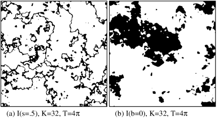
FIG. 16.: Cross sections of two models based on spectrum I. This figure shows the roughness of the interface for large $K$ (Compare Figs. 7(i) & (d)).

of singular behaviour implies a fractal surface. The fractal dimension ‘$D_{s}$’ is given in terms of the correlation function through the relation $p_{2}(r)\simeq p-cr^{3-D_{s}}$ with $c$ some constant. We infer from Eqn. (B4) that our Model I $(\epsilon=1/2)$ has a fractal surface with $D_{s}=2.5$.

As discussed in [20] it is necessary to introduce a finite-cutoff wave number $K$ for computational and physical reasons. We now show how this parameter changes the microstructure. The wave-number $K$ corresponds to a cut-off wavelength $\lambda_{min}=2\pi/K$ which specifies the scale of the smallest “ripples” on the surface. Thus we expect the surface area to scale as a fractal down to some length scale related to $\lambda_{min}$. This can be confirmed mathematically by considering the small $r$ behaviour of $p_{2}(g_{\mbox{$K$}}(r))$.

For arbitrary $r$, $g_{\mbox{$K$}}(r)$ can be expressed in terms of the moments of $k$. Using a Taylor series expansion for $\sin kr$ in the definition of $g_{\mbox{$K$}}$ (2) we have

$$g_{\mbox{$K$}}(r) = 1-\frac{1}{6}\left({\int_{0}^{K}4\pi\rho_{\mbox{$K$}}(k){k^{4}}dk}\right)r^{2}+O(K^{3}r^{2})$$ (B5)

$$\approx 1-\frac{1}{6}\langle k^{2}\rangle r^{2},$$ (B6)

where the latter approximation is valid if $r\ll\lambda_{min}$. Substituting this result into the expansion for $p_{2}$ (B3) and using relation (B1) gives [21, 28]

$$\frac{S}{V}=\frac{2}{\pi}\sqrt{\frac{\langle k^{2}\rangle}{3}}\left({e^{-\frac{1}{2}{\alpha^{2}}}+e^{-\frac{1}{2}{\beta^{2}}}}\right).$$ (B7)

Thus for $r\ll\lambda_{min}$ the surface is behaving in a regular manner ($D_{s}=2$) as anticipated. Note that for the case $K\to\infty$ and $\epsilon<1$ the moment $\langle k^{2}\rangle$ diverges and this approximation does not apply.

To examine the behaviour for $r>\lambda_{min}$ we can successively integrate (2) by parts [20] to obtain

$$g_{\mbox{$K$}}(r) \simeq \frac{g_{\infty}(r)}{P}$$ (B9)

$$-\frac{a}{PK^{2\epsilon}}\left({\frac{\cos Kr}{K^{2}r^{2}}+\frac{3\sin Kr}{K^{3}r^{3}}+O(K^{-4}r^{-4})}\right).$$

If $Kr>1$ this expansion is asymptotic to $g_{\mbox{$K$}}$ [54]. Now in the region $\lambda_{min}\ll r\ll 1$ the algebraic terms in the expansion are negligible and $g_{\mbox{$K$}}\simeq g\simeq(1-br^{2\epsilon})/P$ (with $P\simeq 1$).

In summary we have

$$p_{2}(r)\approx\left\{\begin{array}[]{rl}{p-\left({\sqrt{\frac{1}{3}\langle k^{2}\rangle}\frac{f(1)}{2\pi}}\right)r}&{0\leq r\ll\lambda_{min}}\\ {p-\left({\sqrt{2b}\frac{f(1)}{2\pi}}\right)r^{\epsilon}}&{\lambda_{min}\ll r\ll 1}.\end{array}\right.$$ (B10)

This demonstrates the regular ($D_{s}=2$) nature of the surface in the former region, and the fractal behaviour ($D_{s}=3-\epsilon$) over the spatial scales in the latter region.

C Intersection volume of two and three spheres

The intersection volume $V^{(2)}_{I\mu\nu}(d)$ of two spheres of radii $\mu$ and $\nu$ separated by a distance $d$ is simple to calculate. With $r_{1}=\min(\mu,\nu)$ and $r_{2}=\max(\mu,\nu)$ $V^{(2)}_{I}=4\pi r_{1}^{3}/3$ if $0\leq d<r_{2}-r_{1}$, $V^{(2)}_{I}=0$ if $r_{2}+r_{1}\leq d<\infty$ and

$$V^{(2)}_{I}=2\pi(r_{1}^{3}+r_{2}^{3})/3-\pi(r_{1}^{2}x_{1}+r_{2}^{2}x_{2}-\frac{1}{3}x_{1}^{3}-\frac{1}{3}x_{2}^{3})$$ (C1)

if $r_{2}-r_{1}\leq d<r_{2}+r_{1}$. Here $x_{1}=(d^{2}+r_{1}^{2}-r_{2}^{2})/(2d)$ and $x_{2}=d-x_{1}$.

A compact form of the intersection volume of three spheres of equal radii ($r=1$) has been derived previously by Powell [55]. Several of the key simplifications in the derivation formula are not possible when the spheres have different radii. However a less elegant but straight forward result can be determined. Suppose the spheres have radii $r_{A}$, $r_{B}$ and $r_{C}$ and are distances $a$, $b$ and $c$ apart and that there exist two unique points $P$ and $Q$ where the surface of the spheres meet. From Powell [55] the intersection volume of the three spheres is equal to twice the following expression (Powell’s Theorem):

	The volume of the tetrahedron PABC
$-$	The volume of the sphere center A enclosed by the faces of the tetrahedron PABC which meet at A
$-$	The volume of the sphere center B enclosed by the faces of the tetrahedron PABC which meet at B
$-$	The volume of the sphere center C enclosed by the faces of the tetrahedron PABC which meet at C
$+$	The intersection volume of the spheres centered at B and C enclosed by the two faces of the tetrahedron PABC which meet in BC
$+$	The intersection volume of the spheres centered at C and A enclosed by the two faces of the tetrahedron PABC which meet in CA
$+$	The intersection volume of the spheres centered at A and B enclosed by the two faces of the tetrahedron PABC which meet in AB

FIG. 17.: Geometrical elements used in the calculation of the intersection volume of three spheres of different radii. The axis and nomenclature are those employed in the text. (a) the tetrahedron base; (b) the sphere centered at $A$ enclosed by three faces of the tetrahedron.

The cases where there is no unique point of intersection between the spheres is discussed below. We first define a coordinate system with origin at the center of sphere $C$ as drawn in Fig. 17(a). By solving the equations of the three spheres simultaneously it is simple to show that

$$x_{P} = {{{a^{2}}-{{r_{B}}^{2}}+{{r_{{\rm C}}}^{2}}}\over{2\,a}}$$ (C2)

$$y_{P} = \frac{-b^{2}+r_{A}^{2}-r_{C}^{2}+2b\cos Cx_{P}}{2b\sin C}$$ (C3)

$$z_{P} = \sqrt{r_{C}^{2}-x_{P}^{2}-y_{P}^{2}}.$$ (C4)

It is also necessary to know the distances $a_{B},a_{C}\dots$ given in Fig. 17(a). We have $a_{C}=(a^{2}+r_{C}^{2}-r_{B}^{2})/(2a)$, $b_{A}=(b^{2}+r_{A}^{2}-r_{C}^{2})/(2b)$ $c_{B}=(c^{2}+r_{B}^{2}-r_{A}^{2})/(2c)$, $a_{B}=a-a_{C}$, $b_{A}=b-b_{C}$ and $c_{A}=c-c_{B}$.

The volume of the tetrahedron is $V_{T}=\frac{1}{6}ab\sin Cz_{P}$. The solid angle $\phi_{A}$ of the tetragonal wedge at A (see Fig. 17(b)) can be calculated by using the fact that $\phi_{A}=(E+F+D-\pi)$ and

$$\cos D=\frac{\cos d-\cos e\cos f}{\sin e\sin f}$$ (C5)

(similarly for $\cos E$ and $\cos F$). This gives

FIG. 18.: Several of the topologically distinct cases which arise in the calculation of the intersection volume of three spheres of different radii.

$$\phi_{A} = \cos^{-1}\left({\frac{c_{A}-\cos Ab_{A}}{\sin A\sqrt{r_{A}^{2}-b_{A}^{2}}}}\right)$$ (C8)

$$+\cos^{-1}\left({\frac{r_{A}^{2}\cos A-b_{A}c_{A}}{\sqrt{r_{A}^{2}-b_{A}^{2}}\sqrt{r_{A}^{2}-c_{A}^{2}}}}\right)$$

$$+\cos^{-1}\left({\frac{b_{A}-\cos Ac_{A}}{\sin A\sqrt{r_{A}^{2}-c_{A}^{2}}}}\right)-\pi.$$

Similar results are obtained for the solid angles $\phi_{B,C}$.

It is critical to know whether the point $x_{P},y_{P}$ lies inside or outside each of the faces of the triangle. This can be done by defining the variables

$$s_{A} = {\rm sgn}(-y_{P})$$ (C9)

$$s_{B} = {\rm sgn}(\cos Cy_{P}+\sin Cx_{P})$$ (C10)

$$s_{C} = {\rm sgn}(\cos By_{P}-\sin Bx_{P}+a\sin B).$$ (C11)

Then for example $s_{A}=\pm 1$ as the point $(x_{P},y_{P})$ is inside or outside face $a$ of the triangle $ABC$. In the case $r_{A}=r_{B}=r_{C}=1$ (Powell [55]) we have $x_{P}=a/2$ and $y_{P}=-c\cos A/2\sin C$ so that $s_{A}={\rm sgn}(\cos A)$, $s_{B}={\rm sgn}(\cos B)$ and $s_{C}={\rm sgn}(\cos C)$ as they should.

The wedge angle associated with the intersection volume of spheres B & C is,

$$\theta_{A}=\cos^{-1}\left({s_{A}\frac{\sqrt{r_{B}^{2}-a_{B}^{2}-z_{P}^{2}}}{\sqrt{r_{B}^{2}-a_{B}^{2}}}}\right).$$ (C12)

Similarly for the angles $\theta_{B}$ & $\theta_{C}$.

Now the volume of a tetragonal wedge of solid angle $\phi$ is $r^{3}\phi/3$ and the intersection volume of spheres enclosed in a wedge of angle $\theta$ is $\theta V^{(2)}_{I}/2\pi$. Therefore, by Powell’s theorem,

$$V_{Ixyz}^{(3)}(a,b,c) = 2V_{T}-\frac{2}{3}x^{3}\phi_{A}-\frac{2}{3}y^{3}\phi_{B}-\frac{2}{3}z^{3}\phi_{C}$$ (C14)

$$+\frac{\theta_{A}}{\pi}V^{(2)}_{Iyz}(a)+\frac{\theta_{B}}{\pi}V^{(2)}_{Ixz}(b)+\frac{\theta_{C}}{\pi}V^{(2)}_{Ixy}(c).$$

Here $x=r_{A}$, $y=r_{B}$ & $z=r_{C}$. This formula is equivalent to Powell’s result [55] in the case $x=y=z=1$.

Several other cases arise if the point $P$ does not exist. Some of these are illustrated in Fig. 18. Either two (or more) of the spheres are disconnected (not illustrated), they are connected but $Va^{(3)}_{I}=0$ (b) or the intersection volume is given by that of two of the spheres (c) or some other formula (d).

D Derivation of $\zeta_{1}|_{p=0}$ (IOSA)

It is possible to develop an independent check on the calculation of $\zeta_{1}$ for the IOSA model by direct calculation of $\sigma_{e}$. Using the framework of Reynolds and Hough [56] gives

$$\sigma_{e}=\sigma_{2}+(\sigma_{1}-\sigma_{2})pf_{1}$$ (D1)

where $f_{1}=\bar{E}_{1}/\bar{E}$. Here $\bar{E}_{1}$ is the average of the field throughout phase 1 and $\bar{E}$ is the applied field. While the above formula is exact it is only possible to evaluate $E_{1}$ approximately. In the low concentration regime ($p\ll 1$) $E_{1}$ is the field within a hollow sphere (conductivity $\sigma_{1}$) embedded in an infinite medium (conductivity $\sigma_{2}$) subject to an applied field $\bar{E}$. To determine this field we consider a more general problem where the conductivities of the innermost spherical region ($0\leq r<r_{0}$), the annulus ($r_{0}\leq r<r_{1}$) and the enclosing medium ($r_{1}\leq r<\infty$) are $\sigma_{a}$, $\sigma_{b}$ and $\sigma_{c}$ respectively. The potential of the field satisfies Laplace’s equation and charge conservation boundary conditions at phase boundaries. Using standard techniques it is possible to show that, in each region, the potential has the form $\phi_{d}=(A_{d}r+B_{d}r^{-2})\cos\theta$ with $d=a,b$ or $c$. Applying the appropriate boundary conditions on each of the faces of the hollow sphere gives,

$$A_{a} = -9s^{3}\bar{E}/H;\;\;B_{a}=0;\;\;A_{b}=-3s^{3}\bar{E}(2+x)/H;$$ (D2)

$$B_{b} = -3r_{1}^{3}\bar{E}(1-x)/H;\;\;A_{c}=-\bar{E};$$ (D3)

$$B_{c} = -r_{1}^{3}\bar{E}[(1-x)(1+2y)+s^{3}(2+x)(1-y)]/H.$$ (D4)

where $H=2(1-x)(1-y)+s^{3}(2+x)(2+y)$, $x=\sigma_{a}/\sigma_{b}$, $y=\sigma_{b}/\sigma_{c}$ and $s=r_{1}/r_{0}$. For the desired value of $f_{1}$, $\sigma_{a}=\sigma_{c}=\sigma_{2}$ and $\sigma_{b}=\sigma_{1}$. Considering volume averages of the field lead to

$$(f_{1})_{z}=-\frac{A_{b}}{\bar{E}}=\frac{3s^{3}\sigma_{2}(2\sigma_{1}+\sigma_{2})}{s^{3}(2\sigma_{1}+\sigma_{2})(2\sigma_{2}+\sigma_{1})-2(\delta\sigma)^{2}},$$ (D5)

where $\delta\sigma=\sigma_{1}-\sigma_{2}$ and $(f_{1})_{x}=(f_{1})_{y}=0$. Now expanding Eqn. (D1) in powers of $\delta\sigma$ gives,

$$\sigma_{e}\simeq\sigma_{2}+(\delta\sigma)p-\frac{1}{3\sigma_{2}}(\delta\sigma)^{2}p+\frac{2+s^{3}}{9s^{3}\sigma_{2}^{2}}(\delta\sigma)^{3}p.$$ (D6)

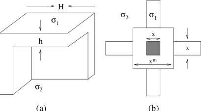
FIG. 19.: Periodic cellular models: (a) Sheet-like cell; (b) Bond/node-like cell.

Similarly Brown’s formula [57] to the same order gives,

$$\sigma_{e}\simeq\sigma_{2}+(\delta\sigma)p-\frac{1}{3\sigma_{2}}(\delta\sigma)^{2}p+\frac{1+2\zeta_{1}}{9\sigma_{2}^{2}}(\delta\sigma)^{3}p.$$ (D7)

Equating similar terms leads to $\zeta_{1}|_{p=0}=s^{-3}=r_{0}^{3}/r_{1}^{3}$. Points representing this result are plotted in Fig. 8 and confirm prior calculations of $\zeta_{1}$. It should also be possible to calculate the first order correction, ${\partial\zeta_{1}}/{\partial p}|_{p=0}$, by calculating $\sigma_{e}$ to $O(p^{2})$ [40, 58]. Since $\zeta_{1}$ is observed to have a linear behaviour over a wide range of $p$ [40] (see Fig. 8) this would provide a good estimate of $\zeta_{1}$. Also note that $\eta_{1}|_{p=0}$ can be derived using similar methods.

E Periodic cell models

To explicitly demonstrate the effect of pore shape on effective conductivity we estimate $\sigma_{e}$ for several periodic networks exhibiting sheet-like, grid-like and node/bond-like cells. Consider a structure comprised of periodic repetitions of the unit cell shown in Fig. 19(a). Defining $x=h/H$ the volume fractions of each phase are given by $p=1-(1-x)^{3}\simeq 3x$ and $q=(1-x)^{3}\simeq 1-3x$. Consider the behaviour of the model if $\sigma_{1}\gg\sigma_{2}$. In this case most of the current would flow through the solid faces of the cell which are aligned in the direction of current flow. The volume fraction of these elements of the cell is $p_{1}=2x-x^{2}$. The remaining current would pass through a layer of phase 1 (volume fraction $p_{2}=x(1-x)^{2}$) and the cell core of phase 2 (volume fraction $q$). Treating each of these mechanisms as conductors in parallel we have $\sigma_{e}=p_{1}\sigma_{1}+(p_{2}+q)\sigma^{*}$, where $\sigma^{*}$ is conductivity of the central leakage pathways. Assuming each of the elements of these pathways act as conductors in series gives $\sigma^{*}=(p_{2}+q)(p_{2}\sigma_{1}^{-1}+q\sigma_{2}^{-1})^{-1}$. This leads to

$$\sigma_{e} = (2x-x^{2})\sigma_{1}+\frac{(1-x)^{2}\sigma_{2}}{x(\sigma_{2}/\sigma_{1})+(1-x)}$$ (E1)

$$\simeq \sigma_{2}+\frac{2}{3}p\sigma_{1}-\frac{1}{3}p\sigma_{2}\left({1+\frac{\sigma_{2}}{\sigma_{1}}}\right)$$ (E2)

where the approximation holds for $p\ll 1$. Finally, $\sigma_{e}\simeq\frac{2}{3}\sigma_{1}p$ in the case $\sigma_{2}=0$.

In a similar way a ‘toy’ model can be defined to qualitatively demonstrate the effect that necks/throat have on the effective conductivity. A cross section of the unit cell of a node/bond model is shown in Fig. 19(b). The central cube has side length $x^{m}$ and the six arms have a square cross section of side length $x$. Taking the cell to have unit width we have: $p=x^{3m}+3(1-x^{m})x^{2}$ ($m\leq 1$) and $q=1-p$. If $\sigma_{2}=0$ then most of the current will flow through the bonds parallel to the direction of the applied field. Therefore, $\sigma_{e}\simeq\sigma_{1}x^{2}$. In the case $m=1$ a uniform grid results and $\sigma_{e}\simeq\frac{1}{3}p\sigma_{1}$ to leading order in $p$. For $m=1/3$ a node/bond geometry results and $\sigma_{e}\simeq p^{2}\sigma_{1}$.

REFERENCES

- [1]
- [2]
- [3] S. Torquato, Appl. Mech. Rev. 44, 37 (1991).
- [4] M. B. Isichenko, Rev. Mod. Phys. 64, 961 (1992).
- [5] M. Sahimi, Rev. Mod. Phys. 65, 1393 (1993).
- [6] L. Gibson and M. Ashby, Cellular Solids: Structure and Properties (Pergamon Press, Oxford, 1988).
- [7] F. Gubbels et al., Macromolecules 27, 1972 (1994).
- [8] S. Torquato, Appl. Mech. Rev. 47, S29 (1994).
- [9] M. Beran, Nuovo Cimento 38, 771 (1965).
- [10] M. Beran and J. Molyneux, Q. Appl. Math. 24, 107 (1966).
- [11] J. J. McCoy, Recent Advances in Engineering Science (Gordon and Breach, New York, 1970), pp. 235–254.
- [12] G. W. Milton, J. Appl. Phys. 52, 5294 (1981).
- [13] G. W. Milton and N. Phan-Thien, Proc. Roy. Soc. London A 380, 305 (1982).
- [14] G. W. Milton, Phys. Rev. Lett. 46, 542 (1981).
- [15] P. B. Corson, J. Appl. Phys. 45, 3159 (1974).
- [16] P. M. Adler, C. G. Jacquin, and J.-F. Thovert, Water Resources Research 28, 1571 (1992).
- [17] J. G. Berryman and S. C. Blair, J. Appl. Phys. 60, 1930 (1986).
- [18] M. N. Miller, J. Math. Phys. 10, 1988 (1969).
- [19] R. C. McPhedran and G. W. Milton, Appl. Phys. A 26, 207 (1981).
- [20] A. P. Roberts and M. Teubner, Phys. Rev. E 51, 4141 (1995).
- [21] N. F. Berk, Phys. Rev. Lett. 58, 2718 (1987).
- [22] P.-Z. Wong, J. Koplik, and J. P. Tomanic, Phys. Rev. B 30, 6606 (1984).
- [23] Y. Bernabe, Geophysics 56, 436 (1991).
- [24] R. B. Saeger, L. E. Scriven, and H. T. Davis, Phys. Rev. A 44, 5087 (1991).
- [25] J. N. Roberts and L. Schwartz, Phys. Rev. B 31, 5990 (1985).
- [26] J. A. Quiblier, J. Colloid Interface Sci. 98, 84 (1984).
- [27] N. F. Berk, Phys. Rev. A 44, 5069 (1991).
- [28] M. Teubner, Europhys. Lett. 14, 403 (1991).
- [29] D. J. Green, J. Am. Ceram. Soc. 68, 403 (1985).
- [30] R. Li and K. Sieradzki, Phys. Rev. Lett. 68, 1168 (1992).
- [31] N. C. Wardlaw, Amer. Assoc. Petroleum Geologists Bulletin 60, 245 (1976).
- [32] A. P. Roberts and M. A. Knackstedt, J. Mat. Sci. Lett. 14, 1357 (1995).
- [33] M. A. Knackstedt and A. P. Roberts, Macromolecules 29, 1369 (1996).
- [34] P.-Z. Wong, J. Howard, and J.-S. Lin, Phys. Rev. Lett. 57, 637 (1986).
- [35] H. L. Weissberg, J. Appl. Phys. 34, 2636 (1963).
- [36] S. Torquato and G. Stell, J. Chem. Phys. 79, 1505 (1983).
- [37] Y. C. Chiew and E. D. Glandt, J. Colloid Interface Sci. 99, 86 (1984).
- [38] G. Stell and P. A. Rikvold, Chem. Eng. Comm. 51, 233 (1987).
- [39] C. G. Joslin and G. Stell, J. Appl. Phys. 60, 1610 (1986).
- [40] J. F. Thovert, I. C. Kim, S. Torquato, and A. Acrivos, J. Appl. Phys. 67, 6088 (1990).
- [41] G. E. Pike and C. H. Seager, Phys. Rev. B 10, 1421 (1974).
- [42] J. Kertesz, J. Phys. Lett. (Paris) 42, L393 (1981).
- [43] A. P. Roberts, Ph.D. thesis, Dept. of Applied Mathematics, A.N.U., 1995.
- [44] L. M. Schwartz, P. N. Sen, and D. L. Johnson, Phys. Rev. B 40, 2450 (1989).
- [45] R. M. Christensen, J. Mech. Phys. Solids 38, 379 (1990).
- [46] T. T. Wu, Int. J. Solids Structures 2, 1 (1966).
- [47] L. J. Gibson and M. F. Ashby, Proc. Roy. Soc. Lond. A 382, 43 (1982).
- [48] A long standing problem has been determining the physical significance of the microstructure parameters [14, 18] . Any such interpretation is immediately limited by the fact that for all statistically symmetric media [10, 57]. For example, both phases of the 1-cut GRF models are statistically identical at , but the microstructure can vary widely for different spectra [20]. A further problem in understanding the parameters is that they do not appear to sharply distinguish between percolative and non-percolative composites.
- [49] A. P. Roberts and M. A. Knackstedt (unpublished).
- [50] A. Helte, Proc. R. Soc. Lond. A 450, 651 (1995).
- [51] M. C. Wang and G. E. Uhlenbeck, Rev. Mod. Phys. 17, 323 (1945).
- [52] P. Debye, H. R. Anderson, and H. Brumberger, J. Appl. Phys. 28, 679 (1957).
- [53] H. D. Bale and P. W. Schmidt, Phys. Rev. Lett. 53, 596 (1984).
- [54] J. D. Murray, Asymptotic analysis (Clarendon, Oxford, 1974).
- [55] M. J. D. Powell, Mol. Phys. 7, 591 (1964).
- [56] J. A. Reynolds and J. M. Hough, Proc. Phys. Soc. (London) B70, 769 (1957).
- [57] W. F. Brown, J. Chem. Phys. 23, 1514 (1955).
- [58] D. J. Jeffrey, Proc. Roy. Soc. Lond. A 335, 355 (1973).
- [59] I. C. Kim and S. Torquato, J. Appl. Phys. 71, 2727 (1992).
- [60]