Attractive forces between anisotropic inclusions in the membrane of a vesicle

Abstract

The fluctuation-induced interaction between two rod-like, rigid inclusions in a fluid vesicle is studied by means of canonical ensemble Monte Carlo simulations. The vesicle membrane is represented by a triangulated network of hard spheres. Five rigidly connected hard spheres form rod-like inclusions that can leap between sites of the triangular network. Their effective interaction potential is computed as a function of mutual distance and angle of the inclusions. On account of the hard-core potential among these, the nature of the potential is purely entropic. Special precaution is taken to reduce lattice artifacts and the influence of finite-size effects due to the spherical geometry. Our results show that the effective potential is attractive and short-range compared with the rod length $L$. Its well depth is of the order of $\kappa/10$, where $\kappa$ is the bending modulus.

I Introduction

Lipid membranes are interesting systems in statistical physics and are the subject of many theoretical and experimental investigations because of the abundance of effects they exhibit. Often fluid membranes are considered, which feature the unusual combination of finite bending stiffness and vanishing in-plane shear stress. This is caused by the constituent lipid molecules which can be sheared against each other, but resist bending normal to the plane [1].

Biological membranes also contain inclusions, i. e. impurities that differ from lipid molecules chemically and mechanically. Inclusions are embedded in the membrane and can diffuse laterally. Examples range from rather large inclusions such as proteins and polymers to very small bodies such as so-called gemini comprising two lipid molecules whose head groups are chemically bonded [2]. In general, any membrane component that deviates in its mechanical properties from lipid molecules will be called inclusion. Most of these are rather rigid and thus, the presence of an inclusion locally stiffens the ambient membrane. Inclusions diffuse within the membrane with typical speeds of a few microns per second [2].

Forces between membrane inclusions currently receive considerable interest [3, 4, 5, 6, 7, 8]. They can be divided into two classes, direct forces due to electrostatic and van der Waals interactions, and indirect forces which are mediated by membrane fluctuations. The latter are of interest here. However, indirect fluctuation forces between membrane inclusions should not be confused with depletion forces [9, 10] (although both are entropic in origin) that exist when small particles are depleted from the gap between bigger ones. Indirect inclusion interactions were investigated theoretically, both for isotropic (rotationally invariant in the membrane plane) [3, 4, 5, 11, 12], anisotropic (e. g. rod-like) inclusions [5, 6], and under lateral membrane tension [8]. The above quoted contributions focus on the range $\xi\gg s\gg L$, where $s$ is the center-center distance between two inclusions whose linear, in-plane size is $L$, see Figure 1, and $\xi$ is the persistence length, that is the distance in the membrane over which the correlation of the surface normals decays [4]. Based upon perturbative approaches, it was found that there is an (attractive) long-range interaction potential of the form $\Phi\propto-{k_{\rm B}T}\;(L/s)^{4}$, both for isotropic [4] and anisotropic [5, 6] inclusions ($k_{\rm B}$ and $T$ are Boltzmann’s constant and temperature, respectively). However, its magnitude was predicted to be much smaller than ${k_{\rm B}T}$ over the range of $s\gg L$.

Short range attractive interactions ($s<L$) have been predicted by Netz [7] who treated the interactions between stiff inclusions in a membrane analytically. For his model Netz obtains a logarithmically decaying, attractive interaction potential whose magnitude increases with increasing membrane stiffness (see Sec. II,V). Other studies dealing with short-range interactions between membrane inclusions were performed by Dan et al. [13] and Aranda-Espinoza et al. [14] who considered membrane Hamiltonians with contributions from compression (expansion), spontaneous curvature of the membrane, and bending stiffness. These calculations have been carried out in the limit of vanishing temperature where membrane fluctuations do no longer exist. Also, $s$ in [13, 14] is typically of the order of the membrane thickness, whereas the papers [4, 5, 6] assume a thickness much smaller than $s$.

The present paper is also concerned with short-range interactions but between rod-like inclusions for $s\approx L$ embedded in the surface of a vesicle. Throughout this paper we are exclusively concerned with the case of zero spontaneous curvature. To the best of our knowledge, numerical simulations for three-dimensional fluctuating membranes with finite bending stiffness and inclusions, which are considered here, have not yet been carried out.

The remainder of this paper is organized as follows. Model and simulation algorithm are detailed in Sec. II. In Sec. III, pair distribution functions are introduced. Details of their numerical determination are presented in Sec. IV. Sec. V is devoted to a presentation of the results obtained in this work. The paper concludes in Sec. VI with a summary and discussion.

FIG. 1.: Curved membrane with two rod-like surface inclusions of length $L$ and width $\epsilon\ll L$, separated by the center-to-center distance $s$. The rods are rotated by the in-plane angles $\theta_{1},\theta_{2}$ against the connection vector. Sketches a) and b) show two rods in parallel settings. A perpendicular arrangement similar to c) will be called “T-formation”, a setting such as d) “in-line formation”.

II The Model

The approximations employed in [4, 5, 6] are only valid in the range $s\gg L$ and break down for the interesting case of $s\approx L$. Also, the membrane can no longer be regarded as a continuous surface, as the discrete lipid network becomes more and more influential. Hence, numerical simulations are required to obtain quantitative results. In this regard the Monte Carlo method provides a particularly powerful technique by which thermophysical properties of equilibrium systems can be computed in a rather simple and straightforward manner [15].

The model membrane consists of $N$ hard spheres of diameter $a$, connected by rigid bonds (tethers) of length $r$ with $a\leq r\leq\sqrt{3}a$. This model has been employed previously [16, 17, 18, 19]. Membrane fluidity is realized by the bond-flip algorithm first proposed in [20]. On a closed triangular network, each bond can be regarded as one of the diagonals in the quadrilateral formed by the four surrounding bonds. The bond-flip algorithm rotates the bond within this quadrilateral, so that it represents the other diagonal after the operation. This method allows for vertex diffusion, as any triangulation can be transformed into any other [20]. The bending energy is computed from the Helfrich Hamiltonian [21] by integrating over the surface $S$

$${\cal H}=\int\!{\rm d}S\left(\frac{\kappa}{2}H^{2}+\bar{\kappa}K\right)\;,$$ (1)

where $H\equiv c_{1}+c_{2}$ is the sum of the principal curvatures on the surface, $K\equiv c_{1}\>c_{2}$ the Gaussian curvature, and $\kappa,\bar{\kappa}$ are, respectively, the bending modulus and the Gaussian modulus. The term $\int\!{\rm d}S\;K$ is constant in fixed surface topology due to the Gauß-Bonnet theorem [21]. The term $\int\!{\rm d}S\;H^{2}$ is discretized as in [17],

$$\frac{\kappa}{2}\int\!{\rm d}S\;H^{2}\approx 4\pi\,\kappa+\sqrt{3}\,\kappa\sum_{i=1}^{N_{B}}\bigl{(}1-{\bf n}_{\triangle_{a}}{\bf n}_{\triangle_{b}}\,\bigr{)}\;,$$ (2)

where the sum runs over all $N_{B}=3(N-2)$ bonds in the network. Each bond has two adjacent triangles $\triangle_{a}(i)$ and $\triangle_{b}(i)$, whose outer unit normals are denoted by ${\bf n}_{\triangle_{a}}$ and ${\bf n}_{\triangle_{b}}$.

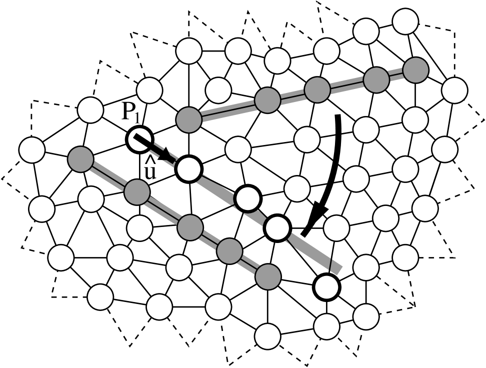
FIG. 2.: Portion of a triangular network of hard spheres with two inclusions, consisting of five vertices each. To the ambient membrane, vertices and bonds within inclusions appear “frozen” and cannot be moved (or flipped) by an MC-step. An inclusion can leap as an entity (arrow) by releasing the old vertices and freezing a new set (bold circles), after having moved the vertices. ${\bf\widetilde{P}}_{1}$ is the position of the selected vertex from which the new rod is tried to be placed along the tangential direction ${\bf\hat{u}}$, see text.

The simulation algorithm consists of two independent parts. The first one follows the one described in [17]. One Monte Carlo step (MCS) consists of attempting to move $N$ randomly selected vertices to new positions within a cube $[-\rho,\rho]^{3}$, centered at their current positions. Next, $N$ bonds are selected and attempted to be flipped. Both processes are accepted or rejected on the basis of their associated change in energy according to the Metropolis algorithm [22].

In addition, mobile, rod-like inclusions are embedded in the membrane. They consist of five rigidly connected hard spheres. None of the spheres in this “frozen” rod-like configuration can be moved independently, nor can the four inner bonds be flipped. A rod and its ambient membrane are thus similar to a spine in which some of the vertebrates are fused. Their biological equivalent would come closest to (multi-)gemini, since the inclusion constituents are equal to those of the plain membrane.

The inclusions can move as an entity, thereby resembling lateral diffusion. This is accomplished by the “rod-leap” algorithm, described below, which is carried out in the second step of the simulation. A new set of five vertices is selected, which may overlap with the old one. To find the new vertices, a random vertex next to the old rod is selected and the four remaining vertices are chosen along the direction of a random unit tangential vector ${\bf\hat{u}}$. Subsequent vertices in the rod must be connected by a bond, as shown in Figure 2. Then a Monte Carlo move is attempted to simultaneously move the last four of the new vertices to the new positions

$${\bf\widetilde{P}}_{n}={\bf\widetilde{P}}_{1}+({\bf\hat{u}}\cdot{\bf P}_{n})\,{\bf\hat{u}}\;,$$ (3)

where ${\bf\widetilde{P}}_{1}={\bf P}_{1}$ is the position of the selected vertex and the ${\bf P}_{n}$, $(n=1\ldots 5)$ are the old vertex positions. The orientation of the local tangential plane next to ${\bf P}_{1}$ is found by averaging all the neighboring triangle normals.

The effect of placing a rod somewhere is to flatten the membrane locally. Note that this does not affect the surface topology. No holes or contact angles at the membrane-inclusion boundary are introduced and hence the Gauß-Bonnet theorem remains valid. If finite contact angles are assumed [8, 12], the number of the inclusions must be kept constant, whereas in the present case the Gauß-Bonnet theorem would remain valid even if the number of inclusions were varied. This flattening effect quenches fluctuations normal to surface of the vesicle. On the other hand, inclusions hardly increase the net bending energy of the ground state vesicle (sphere) of $E_{0}=8\pi\kappa$ [17]. Figure 3 shows a snapshot of a simulation with $N=1012$ vertices.

The total number of vesicle vertices $N$ and number of rods $N_{R}$ must be carefully chosen to ensure that the vesicle is not too strongly perturbed by the rods. Also, the impact of multi-body effects among the rods is crucial for the reliability of the simulations. The rods on the membrane can be considered a lattice gas that should be as dilute as possible. In the present simulation, $N_{R}=4$ rods were placed on a vesicle of $N=1012$ vertices. With this choice, only $2\%$ of the vertices are occupied by inclusions. The average rod length of $L=4\left\langle{r}\right\rangle$, where $\left\langle{r}\right\rangle\approx a(1+\sqrt{3})/2$ is the mean bond length, is only about half as long as the average vesicle radius of gyration that is computed to be $\left\langle{R_{g}}\right\rangle=8.13\left\langle{r}\right\rangle$ for $\kappa/{k_{\rm B}T}=7.5$. An alternative measure of coverage of the membrane by inclusions is obtained by assigning a disk of size $A_{L}=\pi\,(L/2)^{2}$ to each rod. The total area covered by the disks $N_{R}A_{L}/\left\langle{A}\right\rangle$ is about $6\%$ of the average vesicle surface area ($\left\langle{A}\right\rangle\approx 841\left\langle{r}\right\rangle^{2}$). Thus, we conclude that with the above choice of constants, the vesicle is not strongly perturbed by the inclusions and many-body effects are expected to be negligible (see also below).

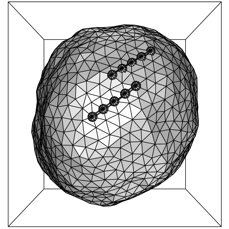
FIG. 3.: Simulation snapshot of a vesicle with $N=1012$ vertices and $\kappa/{k_{\rm B}T}=7.5$. The shades on the surface may be thought of as reflections from a spotlight. Two inclusions with their incorporated spheres are visible on the membrane.

Thermal fluctuations induce a finite effective surface tension $\tau$ in fluid membranes. Therefore, in principle $\tau$ introduces an additional length scale. However, this tension was estimated as $\tau\approx{k_{\rm B}T}\xi^{-2}$ [23] and thus is very small in the regime that is of interest here. In the case of biological membranes, experiments show [24] that the effective surface tension is negligibly small.

III Pair distribution functions

The goal of the present work is the computation of the fluctuation-induced interaction potential of the inclusions $\Phi_{\rm RR}(s,\theta_{1},\theta_{2},\kappa)$. The total energy of a given triangulation ${\cal T}_{N}$, as given by (1) and (2), depends on the positions of the vertices ${\bf X}_{1}\dots\bf X_{N}$ and on the $N\times N$ connectivity (adjacency) matrix $\mathsf{S}$, where ${\mathsf{S}}_{ij}=1$ if vertices $i$ and $j$ are connected by a bond and zero otherwise. The partition function can then be written as [18]

$${\cal Z} = \int\!{\rm d}{{\cal T}_{N}}\;{\exp\bigl{(}-\beta({\cal H}[{\cal T}_{N}]+U_{\rm bond})\bigr{)}}$$ (4)

$$= \sum_{\mathsf{S}}\int\!\Bigl{(}\prod_{i=1}^{N}{\rm d}{\bf X}_{i}\Bigr{)}\>\exp\bigl{(}-\beta({\cal H}[{\cal T}_{N}]+U_{\rm bond})\bigr{)}\;.$$ (5)

Here, $U_{\rm bond}$ is introduced as a constraint imposed on the bonds between neighboring hard spheres forming the membrane. It is zero if all bond lengths $r_{i}$ are in the range $a\leq r_{i}\leq\sqrt{3}a$ and infinite otherwise. In our model, the only effect of adding inclusions to the membrane is to prohibit certain triangulations that do not adhere to the conditions described in the preceding section. In (4), this can be accounted for by extending the definition of $U_{\rm bond}$ so that it diverges also if ${\cal T}_{N}$ cannot accommodate the $N_{R}$ inclusions.

Triangulations can be transformed into each other by means of the bond-flip algorithm and thus no vertex is different from the others. Consequently, the average energy of a triangulation with, say, two inclusions only depends on their mutual distance $s$ and angles $\theta_{1}$, $\theta_{2}$, see Figure 1. This is the basic assumption of the present work. Strictly speaking, the distance $s$ is the length of the shortest geodesic on the surface that connects the centers of the two inclusions. For $s\ll\xi$, however, the Euclidean distance can be taken. The inclusion interaction is purely entropic and not a result of direct molecular interaction. However, an effective interaction potential $\Phi_{\rm RR}(s,\theta_{1},\theta_{2},\kappa)$ can be defined as a potential of mean force (PMF) [25] by the relation

$$\Phi_{\rm RR}+\Phi_{\rm ma}=-{k_{\rm B}T}\,\ln g^{(2)}\;,$$ (6)

where $\Phi_{\rm ma}$ is the mutual avoidance potential of the rods and $g^{(2)}=g^{(2)}\bigl{(}s,\theta_{1},\theta_{2},\kappa\bigr{)}$ is the pair distribution function of the inclusions on the triangulation.

The potential $\Phi_{\rm RR}$ was calculated analytically in [6] for the range $\xi\gg s\gg L$. Surprisingly, the result depends on the sum of the angles $\theta_{1}+\theta_{2}$ between the rods and the connecting vector. However, $\theta_{1}+\theta_{2}$ is the same for the T-formation (Figure 1 c) and, for example, the case $\theta_{1}=\theta_{2}=45^{\circ}$ (Figure 1 b). For small distances $s<L$ that are mainly considered in this article, the latter case is essentially a parallel side-by-side position, and thus parallel and perpendicular relative orientations (Figure 1 a,c) would be indistinguishable. For this reason, the angle difference $\theta:=|\theta_{1}-\theta_{2}|$ is a better variable here for $s\approx L$. On the other hand, one has to take into account that for $s\geq L$, the parallel side-by-side position and e. g. the in-line positions (Figure 1 a,d) are then indistinguishable.

IV Numerical Details

We approximate $g^{(2)}$ by a histogram $g^{(2)}_{ij}$. To do so, a rod pair histogram $n_{ij}$ of $25\times 25$ entries is generated. After regular intervals during the Monte Carlo simulation, all $N_{R}(N_{R}-1)/2$ pairs of the $N_{R}$ rods are considered. If $s\leq s_{\rm max}$, where $s_{\rm max}$ is a cut-off distance small compared to $\langle R_{g}\rangle$, $n_{ij}$ is incremented by one. Here, the indices $i$ and $j$ are rounded to the closest integer $i\simeq 25\;s/s_{\rm max}$ and $j\simeq 25\;\theta/(\pi/2)$ (rods are head-tail symmetrical). For $s_{\rm max}$, a length of $1.5L$ is used. The relationship between $n_{ij}$ and $g^{(2)}_{ij}$ is

$$g^{(2)}_{ij}=\frac{n_{ij}}{n_{\rm tot}}\>\frac{\left\langle{A}\right\rangle}{\left\langle{A_{i}}\right\rangle}\;,$$ (7)

which is valid for $s\leq s_{\rm max}$. Here, $n_{\rm tot}$ is the total number of pairs of rods considered (some of which with $s>s_{\rm max}$ and thus $n_{\rm tot}\geq\sum_{i,j}n_{ij}$), and $\left\langle{A_{i}}\right\rangle$ is the average surface area of a strip on the vesicle with $s\in[i,\>i+1]\!\times\!s_{\rm max}/25$, analogous to the area between two parallels on the globe.

FIG. 4.: If two idealized rods $A$ and $B$ have a center-center distance $\overline{P_{A}\,P_{B}}=s$ of less than $L$, the usual accessible rotational angle of rod $B$ around its center $P_{B}$ of $\pi$ is reduced to $\pi-\alpha=\beta_{a}+\beta_{b}$.

The pair distribution function $g^{(2)}$ is unity for a uniform inclusion distribution on an exactly spherical vesicle. However,
a) the vesicle shape deviates from the sphere especially for small $\kappa$.
b) Since inclusions are bound to vertices, “quantization” effects in the density can be expected if $s$ becomes comparable to $\left\langle{r}\right\rangle$.
c) In addition, a peak in $g^{(2)}$ for $s\approx a$ (the smallest possible distance) can be expected for the following reason: An inclusion straightens a row of vertices, thereby forcing its vicinity to remain closer to the perfect, flat and evenly spaced lattice. Trial moves that consist in placing a rod parallel to an existing one might be less likely to violate a bond length condition because the lattice is more uniform there (closer to the regular hexagonal lattice).
Effects b) and c) are typical lattice artifacts and therefore unphysical. They are eliminated by the procedure outlined below.

We are only interested in the variation in $g^{(2)}$ caused by the increased probability of placing inclusions close to each other, for the membrane there is less corrugated normal to the plane than on average. In order to remove artifacts a-c, normalization runs are performed, according to the following prescription. The rod-leap MC step conforms in all details to the prescription described in the last section, except that before the bending energies of the new and previous rod positions are compared, the new vertices are moved back to their original positions. In other words, in the normalization run, each trial move is accepted if no bonds would be broken in moving the vertices to the positions ${\bf\widetilde{P}}_{n}$, but since vertices are never actually moved there, the lattice remains unchanged. This yields a normalization histogram $\widetilde{n}_{ij}$ and analogous to (7) a pair distribution function $\widetilde{g}^{(2)}$. As a consequence, the moves in the normalization runs share all three types of artifacts a-c, but are insensitive to differences in bending energy. This allows to compute $\Phi_{\rm RR}(s,\theta)$ by

$$\frac{{\Phi_{\rm RR}}_{,\;ij}}{{k_{\rm B}T}}\stackrel{{\scriptstyle~{}}}{{=}}-\ln\frac{\;g^{(2)\;}_{ij}}{\widetilde{g}^{(2)}_{ij}}=-\ln\frac{n_{ij}\;\widetilde{n}_{\rm tot}}{\widetilde{n}_{ij}\;n_{\rm tot}}\;.$$ (8)

Inclusions cannot overlap with others which implies a mutual avoidance condition of $\sin\theta>2s/L$ as shown in Figure 4. Also, the center-center distance cannot be smaller than a hard sphere diameter, $s\geq a$. The mutual avoidance potential $\Phi_{\rm ma}$ from (6) is infinite in these regions and zero elsewhere.

Depletion effects [9, 10] play no role in the present simulation, since the lipids (free vertices) as the “small particles” in the membrane network always retain their uniform density.

V Results

A set of simulation runs is performed with different values for the bending stiffness coefficient $\kappa$. For each simulation, a normalization run is performed according to the prescription outlined above. The simulation length is $10^{8}$ MC-steps. Figure 5 shows $-{\Phi_{\rm RR}}_{,\;ij}(s,\theta)$ for $\kappa/{k_{\rm B}T}=7.5$. The rows in the back of the histogram ($\theta\rightarrow 0$) refer to rod pairs in parallel position; for small $s$, this must be a side-by-side arrangement (Figure 1 a,b). For $s/L\geq 1$, rod pairs in the in-line formation (Figure 1 d) also contribute to the average. The front rows in the diagram ($\theta\rightarrow 90^{\circ}$) refer to rods in the T-formation, which is slightly repulsive for very small $s$. This means that a close, perpendicular position reduces membrane fluctuations most efficiently.

FIG. 5.: Plot of $-\Phi_{\rm RR}(s,\theta)$ for $N=1012$ and $\kappa/{k_{\rm B}T}=7.5$. The plateau on the left side with the shape of the letter ‘h’ is the mutual avoidance area described in Sec. III; $\Phi_{\rm RR}(s,\theta)$ is not defined there and $\Phi_{\rm ma}$ diverges. The peak in the back corresponds to the interactive interaction of parallel side-by-side rod pairs, the slight dip in front to rods in the “T-formation”.

In order to find out about the impact of many-body effects, the fraction of entries $n_{ij}$ stemming from isolated pairs of inclusions to those entries corresponding to clusters of three or more inclusions is calculated. An isolated pair is defined as a pair of inclusions with $s\leq s_{\rm max}$ in the absence of other rods which are closer than $s_{\rm max}$ to either of the two. About $91\%$ of the entries in $n_{ij}$ stem from isolated pairs. Many-body effects are thus negligible in the present simulation as far as the attractive well of the potential is concerned. These results therefore confirm the conjecture stated at the end of Sec. II.

In Figure 6a, $-\Phi_{\rm RR}(s,\theta=0)$ is shown for $\kappa/{k_{\rm B}T}=2.0,\;7.5$, and $11.0$. The decay is very rapid with $\Phi_{\rm RR}$ vanishing approximately at $s/L\approx 0.6$ within the precision of the simulation. At $s/L=0.75=3\left\langle{r}\right\rangle$ and $s/L=1.0=4\left\langle{r}\right\rangle$, remnants of the lattice periodicity induce small peaks in the graphs. The figure shows that $\Phi_{\rm RR}$ is attractive for small distances $s\stackrel{{\scriptstyle~{}}}{{<}}L$, but short-range. Netz [7] found $\Phi_{\rm RR}(s)$ to decay logarithmically. A fit with a logarithmic function of the type given in [7] is shown in Figure 6b . In addition to the short-range attraction there might also be a long-range component. In [6] ${k_{\rm B}T}/128$ was estimated for the magnitude of the leading term of long-range attraction in the effective potential between rodlike inclusions. This value is less than the statistical error of our data in the limit of larger s (see Figure 6).

FIG. 6.: a) Plot of $-\Phi_{\rm RR}(s,\theta=0)$; the graph for $\kappa/{k_{\rm B}T}=7.5$ ($+$) corresponds to the slice from Figure 5 along $s$ at $\theta=0$. The distance between two tics on the abscissa equals one mean bond length $\left\langle{r}\right\rangle$ ($L=4\left\langle{r}\right\rangle$). The vertical dashed line at $s/L=a/L=0.183$ marks the smallest possible bond length. b) as a) but for $\kappa/{k_{\rm B}T}=11.0$ together with a fit of  $a_{1}\ln(1-\exp(-a_{2}s/L))$, ($a_{1}=7.5$, $a_{2}=6.6$) following the theory of Netz [7].

Consequently, our data do not permit us to comment on long-range effective interactions between inclusions. It is, however, noteworthy, that due to the computational method of a perturbative treatment in terms of inverse powers of $s$, the results of [4, 6] cannot rule out the existence of short-range attractions consistent with the present findings. The results in [7], on the other hand, are exact and remain valid in the strong-coupling limit.

The larger $\kappa$, the more attractive becomes the interaction. Figure 7 shows that this relationship is almost linear, with roughly ${\rm max}(-\Phi_{\rm RR}(s,\theta=0))\approx\kappa/10$.

FIG. 7.: Plot of ${\rm max}(-\Phi_{\rm RR}(s,\theta=0))$ for different bending moduli $\kappa$. Inclusions on stiffer membranes feel a more attractive potential, the relationship is roughly linear with ${\rm max}(-\Phi_{\rm RR}(s,0))\approx\kappa/10$.

In other words, the effective attractive interaction between a pair of inclusions becomes stronger the stiffer the membrane of the vesicle is. This may seem contradictory because the stiffer the membrane the more suppressed are fluctuations of the membrane. However, we notice from the work of Netz [7] that short-range interactions between a pair of inclusions may be expected to depend logarithmically on the ratio $s/\xi$ for $s/\xi\ll 1$. A fit of the functional form for $\Phi_{\rm RR}(s)$ proposed by Netz to our data shows that the latter are consistent with a logarithmic decay of the effective potential (see Figure 6b). The correlation length $\xi$, on the other hand, increases with $\kappa$ as $\xi\propto\exp(4\pi\kappa/(3{k_{\rm B}T}))$ [18]. Thus, combining the logarithmic decay of $\Phi_{\rm RR}$ with the latter expressions leads to a linear increase of $-\Phi_{\rm RR}$ with $\kappa$ for fixed $s$ and $T$ which is consistent with the plot in Figure 7.

VI Discussion and Conclusions

The present article discusses Monte Carlo simulations for closed, triangulated membranes with mobile, rod-like inclusions as an extension of a widely used model [16, 17, 18, 19]. Inclusions locally straighten the network, thereby quenching lateral fluctuations. The effective interaction potential is attractive and short-range (see Figure 6). For $s\rightarrow 0$, it is limited by the mutual avoidance condition (Figures 4 and 5).

The contribution of this simulation lies in the focus on small inclusion separations. We find an attractive interaction potential of the order of ${k_{\rm B}T}$ between rods that consist of five rigidly connected hard spheres, for bending coefficients of $\kappa/{k_{\rm B}T}$ of the order of $1-10$ (Figure 6). Furthermore, the magnitude of the well depth of the potential grows almost linearly with $\kappa$, as shown in Figure 7. All of the results presented in this paper are valid in the dilute inclusion limit. The form of the function $\Phi_{\rm RR}$ and its magnitude can be expected to change with higher densities. For very high inclusion densities, segregated phases might exist, one of them largely depleted of inclusions and another, dense phase with a nematic order due to the inclusion anisotropy.

In conclusion, these results have implications for the formation of inclusion clusters. Such aggregation is frequently observed experimentally [26] and in simulation [27]. A number of different driving mechanisms have been proposed, aside from those induced by direct interaction or depletion forces [9, 10]. This includes spontaneous curvature [11], lateral tension [3, 8], and conical inclusion shapes [3, 8, 12]. Fluctuation-induced interactions as considered in [4, 5, 6] focus on the large-separation limit $s/L\gg 1$ and result in interaction potentials $\Phi_{\rm RR}\ll{k_{\rm B}T}$. Although this is of great theoretical interest as it draws an analogy to the quantum-mechanical Casimir effect [28, 29], interaction energies far smaller than ${k_{\rm B}T}$ are of little practical relevance in thermodynamic systems. The present work, in contrast, allows to gain insight into the strongly perturbed, short length-scale region, over distances comparable to both the inclusion length and the lipid head size. This is the crucial length scale in chemical and biological applications.

REFERENCES

- [1] R. Lipowsky, Encyc. Appl. Phys. 23, 199–222 (1998).
- [2] T. Ackermann, Physikalische Biochemie (Springer, Berlin, 1992).
- [3] J. B. Fournier, Phys. Rev. Lett. 76, 4436–9 (1996).
- [4] M. Goulian, R. Bruinsma, and P. Pincus, Europhys. Lett. 22, 145–50 (1993), erratum: Europhys. Lett. 23 (1993), 155.
- [5] J. M. Park and T. C. Lubensky, J. de Phys. I 6, 1217–35 (1996).
- [6] R. Golestanian, M. Goulian, and M. Kardar, Phys. Rev. E 54, 6725–34 (1996).
- [7] R. Netz, J. de Phys. I France 7, 833–52 (1997).
- [8] T. R. Weikl, M. M. Kozlov, and W. Helfrich, Phys. Rev. E 57, 6988–95 (1998).
- [9] K. Yaman, C. Jeppesen, and C. M. Marques, Europhys. Lett. 42, 221–6 (1998).
- [10] B. Götzelmann, R. Evans, and S. Dietrich, Phys. Rev. E 57, 6785–800 (1998).
- [11] R. Netz and P. Pincus, Phys. Rev. E 52, 4114–27 (1995).
- [12] P. G. Dommersnes, J. B. Fournier, and P. Galatola, Europhys. Lett. 42, 233–8 (1998).
- [13] N. Dan, A. Berman, P. Pincus, and S. Safran, J. de Phys. II France 4, 1713–25 (1994).
- [14] H. Aranda-Espinoza, A. Berman, N. Dan, P. Pincus, and S. Safran, Biophys. J. 71, 648–56 (1996).
- [15] M. Schoen, in Computational Methods in Colloid and Interface Science, M. Borowko, ed., (Marcel Dekker, New York, 1999), Chap. Structure and Phase Behavior of Confined Soft Condensed Matter, in press.
- [16] G. Gompper and D. M. Kroll, J. Phys.: Condens. Matter 9, 8795–834 (1997), (review article).
- [17] G. Gompper and D. M. Kroll, J. de Phys. I France 6, 1305–20 (1996).
- [18] J. H. Ipsen and C. Jeppesen, J. de Phys. I France 5, 1563–71 (1995).
- [19] Y. Kantor and D. R. Nelson, Phys. Rev. A 36, 4020–32 (1987).
- [20] U. A. Kazakov, I. K. Kostov, and A. A. Migdal, Phys. Lett. 157 B, 295 (1985).
- [21] W. Helfrich, Z. Naturforsch. 28c, 693–703 (1973).
- [22] M. P. Allen and D. J. Tildesley, Computer Simulation of Liquids (Clarendon Press, Oxford, 1987).
- [23] F. David and S. Leibler, J. de Phys. II France 1, 959–76 (1991).
- [24] F. Brochard and J. F. Lennon, J. de Phys. 36, 1035–47 (1976).
- [25] J. P. Hansen and I. R. MacDonald, Theory of Simple Liquids, 2nd ed. (Academic Press, New York, 1986).
- [26] B. Sternberg and J. Gumpert et al., Bioch. et Biophys. Acta 898, 223–30 (1987).
- [27] M. C. Sabra and O. G. Mouritsen, Biophys. J. 74, 745–52 (1998).
- [28] H. B. G. Casimir, Proc. K. Ned. Akad. Wet. 51, 793 (1948).
- [29] M. Krech, The Casimir Effect in Critical Systems (World Scientific, Singapore, 1994).