Charge Relaxation Resistances and Charge Fluctuations in Mesoscopic Conductors

Abstract

A brief overview is presented of recent work which investigates the time-dependent relaxation of charge and its spontaneous fluctuations on mesoscopic conductors in the proximity of gates. The leading terms of the low frequency conductance are determined by a capacitive or inductive emittance and a dissipative charge relaxation resistance. The charge relaxation resistance is determined by the ratio of the mean square dwell time of the carriers in the conductor and the square of the mean dwell time. The contribution of each scattering channel is proportional to half a resistance quantum. We discuss the charge relaxation resistance for mesoscopic capacitors, quantum point contacts, chaotic cavities, ballistic wires and for transport along edge channels in the quantized Hall regime. At equilibrium the charge relaxation resistance also determines via the fluctuation-dissipation theorem the spontaneous fluctuations of charge on the conductor. Of particular interest are the charge fluctuations in the presence of transport in a regime where the conductor exhibits shot noise. At low frequencies and voltages charge relaxation is determined by a nonequilibrium charge relaxation resistance.
PACS numbers: 72.70.+m, 73.23.-b, 85.30.Vw, 05.45.+b

I Introduction

The dynamics of charge relaxation and the fluctuations of charge represent a basic aspect of electrical conduction theory. In this work we are primarily concerned with a novel transport coefficient which governs the relaxation of excess charge on a mesoscopic conductor towards its equilibrium value and also the time-dependent spontaneous fluctuations of this charge [1]. In a macroscopic conductor the relaxation of excess charge is determined by an $RC$-time constant. Macroscopically, electric fields are screened at the surface of conductors and as a consequence the capacitance $C$ is essentially determined by the geometrical configuration of the conductor. In macroscopic circuits, the resistance is typically taken to be a dc-resistance which can be found by considering a time-independent transport problem. Interestingly, for mesoscopic conductors the capacitance can depend in a significant way on the properties of the mesoscopic conductor and its nearby gates. Even more dramatically, the charge relaxation resistance can not be found by considering a time-independent conduction problem. It is the purpose of this work to present a brief review of such charge relaxation resistances. In particular, we consider the charge relaxation resistance of a mesoscopic capacitor, of a quantum point contact, of a chaotic cavity coupled to single channel leads or to wide quantum point contacts, of a ballistic wire, and of a Hall bar. The charge dynamics is of interest in itself but at low temperature it is also expected to be important to understand dephasing.

At equilibrium the charge on a mesoscopic conductor fluctuates due to thermal agitation and due to zero-point fluctuations in the occupation numbers of the reservoir quantum channels. The low frequency spectrum of the charge fluctuations is precisely related to the charge relaxation resistance. Furthermore, it is interesting to ask about the charge fluctuations on a mesoscopic conductor not only in its equilibrium state but also in the presence of transport. At low voltages such a sample exhibits shot noise due to the granularity of the electric charge. We find that the charge fluctuations in this case are again determined by a non-equilibrium charge relaxation resistance which is a close relative of the equilibrium charge relaxation resistance.

The discussion of charge relaxation resistances is a special topic of a much wider field: the characterization of the dynamic and non-linear behavior of mesoscopic samples. We cite here only a review [2], a few original works[3, 4] and some of the recent works [5, 6, 7, 8, 9, 10, 11, 12, 13] to indicate the breadth of interest in this field.

II The mesoscopic capacitor

Consider the conductor shown in Fig. 1. It consists of a small cavity which is via a lead connected to a reservoir

FIG. 1.: Mesoscopic capacitor connected via a single lead to an electron reservoir and capacitivly coupled to a gate. $V_{1}$ and $V_{2}$ are the potentials applied to the contacts, $U$ is the electrostatic potential of the cavity.

at the potential $V_{1}$ and is capacitively coupled to a back gate at the potential $V_{2}$. Throughout this work we treat the back gate as a macroscopic conductor. We are interested in the current $I(t)$ driven through this structure in response to a voltage oscillation $V(t)=V_{1}(t)-V_{2}(t)$ where $V_{1}(t)$ and $V_{2}(t)$ are the potentials at the contacts $1$ and $2$. We are concerned with linear response and without loss of generality can assume that the voltage is of the form $V(t)=V(\omega)exp(-i\omega t)$. In a macroscopic description we would assume that the dynamic conductance $G(\omega)=I(\omega)/V(\omega)$ of such an arrangement is given by a series combination of a geometrical capacitance $C$ and a resistor with resistance $R$. This gives a conductance $G^{-1}(\omega)=(-i\omega C)^{-1}+R$ which when expanded in powers of $\omega$ has the leading terms

$$G(\omega)=-i\omega C+\omega^{2}C^{2}R+O(\omega^{3})$$ (1)

The first term describes the non-dissipative capacitive response due to the displacement current in the circuit and the second term is a dissipative term determined by the capacitance and the $RC$-time of the circuit.

Consider now a conductor that is in the mesoscopic regime. We consider the zero-temperature limit and investigate phase-coherent transport. We are interested in the low-frequency conductance and are main task is to find the mesoscopic analogues of the transport coefficients $C$ and $R$ in Eq. (1). As for dc-transport we describe the conductor with the help of a scattering matrix ${\bf s}$ which relates the amplitudes of the incoming currents in the mesoscopic conductor to the amplitudes of the out-going currents [2]. Note that for the conductor in Fig. 1 we have only reflection processes. If the potentials applied to the conductors are held fixed (constant in time) the scattering matrix depends on the energy $E$ of the incoming carriers and depends on the equilibrium electrostatic potential $U_{eq}$. Thus we write for the scattering matrix ${\bf s}(E,U_{eq})$. The electrostatic potential is in general a complicated function of position and is function of the dc-voltage difference applied across the capacitor. Thus it is generally a complicated task to find the scattering matrix. Here we proceed by assuming that this task has been accomplished and that ${\bf s}(E,U_{eq})$ is known.

In the presence of a time-dependent voltage the electrostatic potential will also exhibit oscillations. For the linear response regime of interest here the oscillating potential $dU(t)$ represents a small additional contribution to the equilibrium potential and the total potential is $U(t)=U_{eq}+dU(t)$. To find the admittance for the system of interest, we proceed in the following way[1]. First we investigate the response to the oscillating potential at contact $1$ and suppose that the internal potential is held fixed at its equilibrium value $U_{eq}$. In a second step we determine self-consistently the internal oscillating potential $dU(t)$. In a third step we find the current response to this internal oscillating potential. We now consider the simple case, in which the oscillating contribution to the internal potential can be taken to be spatially uniform within the cavity. Instead of solving the full Poisson equation to find the internal potential we then ask that the total excess charge $dQ$ on the mesoscopic capacitor plate is related to the variation of the internal potential by a geometrical capacitance coefficient $C$ such that

$$dQ(\omega)=CdU(\omega).$$ (2)

Note that a description in terms of geometrical capacitances is very often also employed in the discussion of Coulomb blockade effects. We will not here give additional details of the derivation but refer the interested reader to Refs. [1, 2]. In the WKB-limit, we express the transport coefficients of interest with the geometrical capacitance $C$ of Eq. (2) and the matrix

$${\bf{\cal N}}=\frac{1}{2\pi i}{\bf s}^{\dagger}\frac{d{\bf s}}{dE}.$$ (3)

Eq. (3) is the phase-delay matrix of Smith [14]. In the WKB limit[15, 16] the derivative with respect to energy of the scattering matrix is equal to minus the derivative of the scattering matrix with respect to the internal potential $U$, $d{\bf s}/{dE}=-d{\bf s}/{d(eU)}$. The trace of this matrix is the (total) density of states (at constant internal potential) of the mesoscopic structure

$${\cal D}=Tr{\bf{\cal N}}=\frac{1}{2\pi i}Tr\left({\bf s}^{\dagger}\frac{d{\bf s}}{dE}\right).$$ (4)

Eq. (4) is evaluated at the Fermi energy (the electrochemical potential) of the mesoscopic structure.

The capacitance of the mesoscopic structure is now found to be a series combination of the geometrical capacitance and the contribution from the density of states[1]

$$C_{\mu}=Ce^{2}{\cal D}/(C+e^{2}{\cal D}).$$ (5)

The capacitance of the mesoscopic structure is of electrochemical nature. It depends in an explicite manner via the density of states on the properties of the electrical conductor. The ratio of the Coulomb energy $E_{c}=e^{2}/2C$ and the density of states is crucial. If $E_{c}>{\cal D}^{-1}$, then the charging energy is large compared to the mean level spacing $\Delta={\cal D}^{-1}$ and the electrochemical capacitance is equal to the geometrical capacitance $C_{\mu}=C$. If $E_{c}<{\cal D}^{-1}=\Delta$ the Coulomb interaction is weak and the electrochemical capacitance is dominated by the density of states $C_{\mu}=e^{2}{\cal D}$.

Let us next consider the resistance. With the assumption of a uniform electrostatic potential inside the cavity and with the Poisson equation replaced by Eq. (2) we find[1]

$$R_{q}=\frac{h}{2e^{2}}\frac{\mbox{Tr}\left(\cal{N}\cal{N}^{\dagger}\right)}{[\mbox{Tr}({\cal N})]^{2}}.$$ (6)

We call this resistance a charge relaxation resistance. First note that this is not a mesoscopic dc-resistance which would be expressed in terms of transmission probabilities. Instead it is the derivative of the scattering matrix with energy which enters. Second, note that it appears with a resistance quantum which is only half as large as the resistance quantum which determines the plateaus in quantum point contacts and in the quantized Hall effect.

In order to better understand these expressions we assume that the scattering matrix has been brought into diagonal form. We can perform such unitary transformations since the expressions given above depend only on the trace of the matrices involved. Since we deal with a scattering problem which involves only reflections, the diagonal elements of the scattering matrix are of the form

$$s_{nn}=e^{i\phi_{n}}.$$ (7)

Here $\phi_{n}$ is the total phase a carrier accumulates from its entrance into the cavity to its exit from the cavity. $n$ labels the number of eigen channels at the Fermi energy. The density of states Eq. (4) now becomes simply the sum of all energy derivatives of the phases, ${\cal D}=(1/2\pi)\sum_{n}d\phi_{n}/dE$. Since $\tau_{n}=\hbar d\phi_{n}/dE$ is the time a carrier in the n-th eigen channel spends in the conductor $\tau_{D}=(1/N)\sum_{n=1}^{n=N}\hbar d\phi_{n}/dE$ is the average time carriers dwell in the conductor if there are $N$ open quantum channels[15, 16]. Thus the density of states is proportional to the number of open channels at the Fermi energy and is proportional to the average dwell time, ${\cal D}=N\tau_{D}/2\pi\hbar$. If we introduce the Coulomb induced, geometrical relaxation time $\tau_{g}=h/e^{2}C$, the expression for the electrochemical capacitance Eq. (5), can equally well be expressed in terms of $\tau_{g}$ and the average dwell time. For $\tau_{\mu}=(h/e^{2}C_{\mu})$ we find

$$\frac{1}{\tau_{\mu}}=\frac{1}{\tau_{g}}+\frac{1}{N\tau_{D}}.$$ (8)

In a basis in which the scattering matrix is diagonal the charge relaxation resistance is,

$$R_{q} = \frac{h}{2e^{2}}\frac{\left(\sum_{n}(d\phi_{n}/dE)^{2}\right)}{(\sum_{n}(d\phi_{n}/dE))^{2}}.$$ (9)

Thus the charge relaxation resistance is proportional to the sum of the squares of the dwell times divided by the square of the sum of the dwell times,

$$R_{q} = \frac{h}{2e^{2}}\frac{\left(\sum_{n}\tau^{2}_{n}\right)}{[\sum_{n}\tau_{n}]^{2}}.$$ (10)

For the case of a single channel, we see immediately that the charge relaxation resistance is quantized

$$R_{q}=\frac{h}{2e^{2}}.$$ (11)

For a spin degenerate channel the quantized resistance would be $R_{q}={h}/{4e^{2}}$. The factor of two is significant. It is a consequence of the fact that in the mesoscopic conductor shown in Fig. 1 there is only one reservoir conductor interface at which the non-equilibrium carrier distribution inside the conductor must relax to the equilibrium distribution of the the reservoir [1]. We note here only that a doubling of the quantum is obtained for interface resistances: If we subtract the the Landauer resistance $R=(h/e^{2})(1-T)/T$ from the two terminal resistance $R=(h/e^{2})1/T$ the difference is a resistance $(h/e^{2})$ which can be viewed as the sum of two sample reservoir-interface resistances $(h/2e^{2})$ as discussed by Imry [17] and Landauer [18]. A closer examination shows, however, that the interface resistance depends on the way voltages are measured and depends on whether or not we have phase-coherent transport [19, 20]. Another situation in which a doubling of the conductance quantum occurs is the conductance of a hybrid normal and superconducting interface and recently it has been argued that also this doubling is connected less to the fact that we have Andreev scattering but instead to the fact that we have a conductor connected to only one (normal) electron reservoir[21]. Such analogies clearly have their limit: In our case the potential is dynamic and not static. In general, for an $N$-channel lead connecting the mesoscopic capacitor plate and the reservoir, the charge relaxation resistance is not quantized. We note that if both ”plates” of the capacitor are mesoscopic, then the charge relaxation resistance acquires two contributions, one from the connection of each plate to a reservoir[1]. In a such a geometry, in the single channel limit, the charge relaxation resistance is $R_{q}={h}/{e^{2}}$.

The charge relaxation resistance determines the first dissipative term in the expansion of the dynamic conductance in terms of frequency. Via the fluctuation dissipation theorem it must thus also be related to the spontaneous current fluctuations in the capacitor. Indeed, for a voltage controlled circuit, Ref. [1] finds that the noise power spectrum of the equilibrium current fluctuations, $2\pi\delta(\omega+\omega^{\prime})S_{II}(\omega)=(1/2)\langle I(\omega)I(\omega^{\prime})+I(\omega^{\prime})I(\omega)\rangle$ is in the classical limit $kT>\hbar\omega$ given by

$$S_{II}(\omega)=2kT\omega^{2}C^{2}_{\mu}R_{q}.$$ (12)

The current fluctuations are accompaned by fluctuations in the internal potential $U$. Since $dI(\omega)=-i\omega dQ(\omega)$ and $dQ(\omega)=CdU(\omega)$ we find for the fluctuation spectrum of the internal potential $U$,

$$S_{UU}(\omega)=2kT(C_{\mu}/C)^{2}R_{q}.$$ (13)

The ratio $C_{\mu}/C$ tends to $1$ in the limit $E_{c}>>e^{2}{\cal D}$ and tends to $0$ in the limit $E_{c}<<e^{2}{\cal D}$. Note that these fluctuations in the internal potential occur for a voltage controlled circuit, i. e. the voltage measured at the terminals (reservoirs) does not fluctuate. For an infinite external impedance the current does not fluctuate but the voltage measured at the terminals now fluctuates with a low frequency spectrum $S_{VV}(\omega)$. The spectrum of external voltage fluctuations $S_{VV}(\omega)$ is at low frequencies just determined by the charge relaxation resistance alone,

$$S_{VV}(\omega)=2kTR_{q}.$$ (14)

In the quantum limit and in the low frequency limit of interest here, $kT$ is replaced by $\hbar|\omega|$ and thus the current fluctuation spectrum is third order in frequency and the voltage fluctuation spectra are first order in frequency.

We have emphasized that for the derivation of Eq. (6) we have described the potential with a single parameter $U$. A more general formula for the charge relaxation resistance, valid for a general potential landscape $U({\bf r})$ is given in Ref. [22]. Both the nominator and the denominator contain the Coulomb interaction. In such a more general formulation the universality of the charge relaxation resistance in the one-channel limit might be lost. Furthermore in our discussion, electron interactions are treated in the random phase approximation. Especially in the few channel limit, even in the presence of open leads, charge quantization effects might be important [23] and these are neglected in our treatment.

III Charge Relaxation Resistances of Chaotic Cavities

To gain further insight into the physical meaning of the charge relaxation resistance, we consider in this section the charge relaxation resistance of cavities which are in the classical limit chaotic [24, 25]. We consider an ensemble of cavities which all have the same mean level spacing but in which individual members exhibit small fluctuations in their shape. To find the distribution of charge relaxation resistances we need to know how the eigenvalues of the Wigner-Smith matrix are distributed. A description of the statistical distribution of these times was obtained only recently. Fyodorov and Sommers[26] used the supersymmetric sigma model to obtain the distribution of the phase-delay time for a unitary ensemble of cavities connected to a perfect single channel lead. Independently Gopar et al. [27, 28] used a conjecture by Wigner to find the distribution of the delay time for the orthogonal, unitary and symplectic ensemble again coupled to a single channel perfect lead. An important advance was made by Brouwer, Frahm and Beenakker[29] who found the distribution of eigenvalues of the Wigner-Smith matrix for a cavity connected to an N-channel lead. These advances have permitted to investigate the fluctuations in the capacitance coefficient[27, 29] given by Eq. (5). Subsequently, these results were used to find the distribution of the transconductance of a chaotic cavity[30], the thermal conductance[31] and the charge relaxation resistances[32] of chaotic cavities which we now discuss. Before proceeding, we mention only that delay time fluctuations are also of interest in optical wave propagation problems and are a subject of experimental interest[33].

For a cavity coupled to a single channel lead[27] the charge relaxation resistance is according to Eq. (10) universal and given by half a resistance quantum. It is sharp and exhibits no fluctuations from one ensemble member to another. The situation changes if we consider a cavity connected to two perfectly transmitting channels, the case considered by Pedersen, van Langen and the author in Ref. [32]. For $N=2$ we see immediately that

$$R_{q} = \frac{h}{2e^{2}}\frac{\left(\tau^{2}_{1}+\tau^{2}_{2}\right)}{[\tau_{1}+\tau_{2}]^{2}}$$ (15)

takes the maximum value $h/{2e^{2}}$ if one of the eigen values vanishes and takes the minimum value $h/{4e^{2}}$ if both eigenvalues are identical. A typical sample will thus exhibit a charge relaxation resistance between these bounds. Ref. [32] finds for the distribution function $P(R_{q})$ of the charge relaxation resistance

$$P(R_{q})=\left\{\begin{array}[]{ll}4,&\beta=1,\\ 30(1-2R_{q})\sqrt{4R_{q}-1},&\beta=2.\end{array}\right.$$ (16)

Here $\beta=1$ applies to an orthogonal ensemble (no magnetic field) and $\beta=2$ applies to a unitary ensemble in which time-reversal symmetry is broken by a magnetic field. These two distribution functions are shown in Fig. 2.In the orthogonal case the distribution is uniform: every charge relaxation resistance between $R_{q}=h/4e^{2}$ and $R_{q}=h/2e^{2}$ is equally probable. In contrast for a unitary ensemble the limiting cases in which one of the eigenvalues vanishes or in which both eigenvalues are equal is not likely and the distribution function is peaked with a maximum at $R_{q}=h/3e^{2}$.

For cavities connected to a single lead with many quantum channels it is possible to find the charge relaxation

FIG. 2.: Distribution of the charge relaxation resistance of a chaotic quantum dot for the orthogonal ensemble (dashed line) and the unitary ensemble (solid line) line. After Ref. [32]

.

resistance via a $1/N$ expansion. The technique necessary to carry out such expansions is discussed in detail in Ref. [34]. The dynamic conductance of a cavity coupled to contacts with a large number of channels was investigated by Brouwer and the author[35]. In the large channel limit the distribution is gaussian and the charge relaxation is well characterized by its ensemble average value. The ensemble averaged charge relaxation resistance is

$$R_{q} = \frac{h}{2e^{2}}\left(\frac{1}{N}+\frac{2-\beta}{\beta}\frac{1}{N^{2}}+O(\frac{1}{N^{3}})\right).$$ (17)

The term proportional to ${1}/{N^{2}}$ is the weak localization correction from enhanced backscattering. Note that this resistance is quantized only on the average.

IV Charge Relaxation in Two Probe Conductors

A Equilibrium and Nonequilibrium Charge Relaxation

Consider now conductors which are connected to two or more contacts (see Fig. 3). In addition the conductor is coupled capacitively to a gate (or a number of gates) with a (total) geometrical capacitance $C$. Let us label the contact to the gate as $3$. For the ac-transport problem we have then a conductance problem with three contacts. The dynamic conductance $G_{\alpha\beta}(\omega)$ is defined as $dI_{\alpha}(\omega)/dV_{\beta}(\omega)=G_{\alpha\beta}(\omega)$ with $\alpha=1,2,3,$ labelling the contact at which the current is measured and $\beta=1,2,3$ the contact at which the oscillating potential is applied. Thus the dynamic conductance is specified by a three times three conductance matrix.

The two probe conductor acts as a simple mesoscopic capacitor to the gate if we consider the case where the voltages at the contact of the conductor oscillate in synchronism: $dV_{1}(\omega)=dV_{2}(\omega)$. The conductance $G_{33}$ has then the same general form as that of a mesoscopic capacitor $G_{33}(\omega)=-i\omega C_{\mu,33}+\omega^{2}C_{\mu,33}R_{q,33}$ with $C_{33}\equiv C_{\mu}$ the conductor to gate capacitance and $R_{q,33}=R_{q}$, where $C_{\mu}$ and $R_{q}$ are, as we now show, given by Eq. (5) and Eq. (6) obtained above. The scattering matrix which describes the conductor with multiple contacts is specified by matrices ${\bf s}_{\alpha\beta}$ which give the outgoing current amplitudes at contact $\alpha$ in terms of the incident current amplitudes at contact $\beta$. It is useful at this point to introduce the matrices[32]

$${\cal N}_{\delta\gamma}=\frac{1}{2\pi i}\sum_{\alpha}s_{\alpha\delta}^{\dagger}\frac{ds_{\alpha\gamma}}{dE}.$$ (18)

The diagonal element $\delta=\gamma$ represents the contribution to the density of states of carriers injected from contact $\gamma$ and is called the injectance of contact $\gamma$. The off-diagonal elements start to play a role if we are interested in the charge relaxation resistance and in the fluctuations of the charge. Thus the total density of states of the conductor is given by the diagonal elements of this matrix ${\cal D}=\sum_{\gamma}\mbox{Tr}({\cal N}_{\gamma\gamma})$; where the trace is again over all quantum channels. Together with the geometrical capacitance the density of states determines the capacitance of the sample vis-a-vis the gate $C_{\mu,33}\equiv C_{\mu}$ with $C_{\mu}^{-1}=C^{-1}+(e^{2}{\cal D})^{-1}$, i. e. the same result that we have found already for the mesoscopic capacitor. The charge relaxation resistance is $R_{q,33}\equiv R_{q}$ with

$$R_{q} = \frac{h}{2e^{2}}\frac{\sum_{\gamma\delta}\mbox{Tr}\left(\cal{N}_{\gamma\delta}\cal{N}^{\dagger}_{\gamma\delta}\right)}{[\sum_{\gamma}\mbox{Tr}({\cal N}_{\gamma\gamma})]^{2}}.$$ (19)

Note, that this is again the same result as Eq. (6) if we understand the matrix ${\bf s}$ to be composed of all four matrices ${\bf s}_{\alpha\beta}$.

Conductors with two or more probes also permit to drive a current through the conductor. In the zero-frequency and zero-temperature limit, for a small applied voltage $V$, the conductor exhibits shot noise in the transport current. The spectral density of the current fluctuations due to the shot noise can also be expressed with the help of the scattering matrix [36] and is given by $S_{II}(\omega=0)=(e^{2}/h)Tr({\bf s}^{\dagger}_{11}{\bf s}_{11}{\bf s}^{\dagger}_{21}{\bf s}_{21})e|V|$. Here we are in particular interested in the charge fluctuations on the conductor in such a situation. In the zero-temperature, low-frequency limit, if current flow is from contact $1$ to contact $2$, we find for the charge fluctuations to leading order in the applied voltage $V$,

$$S_{QQ}(\omega)=2C_{\mu}^{2}R_{v}|eV|$$ (20)

which defines a non-equilibrium charge relaxation resistance [32]

$$R_{v}=\frac{h}{e^{2}}\frac{\mbox{Tr}\left({\cal N}_{21}{\cal N}^{\dagger}_{21}\right)}{[\sum_{\gamma}\mbox{Tr}({\cal N}_{\gamma\gamma})]^{2}}.$$ (21)

Thus the non-equilibrium noise is determined the non-diagonal elements of the density of states matrix Eq. (18).

FIG. 3.: Two probe conductor connected to two electron-reservoirs and capacitivly coupled to a gate.

by a non-diagonal element of the density of states matrix. If both the frequency and the voltage are non-vanishing we obtain to leading order in $\hbar\omega$ and $V$, $S_{QQ}(\omega)=2C_{\mu}^{2}R(\omega,V)\hbar|\omega|$ with a resistance

$$R(\omega,V)\hbar|\omega|=\left\{\begin{array}[]{ll}R_{q}\hbar|\omega|,&\hbar|\omega|\geq e|V|\\ R_{q}\hbar|\omega|+R_{V}(e|V|-\hbar|\omega|),&\hbar|\omega|\leq e|V|\end{array}\right.$$ (22)

which is a frequency and voltage dependent series combination of the resistances $R_{q}$ and $R_{v}$. If the temperature is non-vanishing and exceeds $\hbar\omega$, Eq. (22) holds with $\hbar\omega$ replaced by $kT$. Below we discuss the resistances $R_{q}$ and $R_{v}$ in detail for several examples: a chaotic cavity, ballistic wires, a Hall bar and a quantum point contact.

B Chaotic Cavities

Since the equilibrium charge relaxation resistance is the sum of equally weighted diagonal density matrix elements the distribution of the charge relaxation resistance shown in Fig. 2 and given by Eq. (16) for the mesoscopic capacitor coupled to a single lead with two quantum channels is also the distribution function for the charge relaxation resistance of a conductor coupled to two leads each supporting one quantum channel. Novel information is, however, obtained if we consider the resistance $R_{v}$ which governs the charge fluctuations in the presence of a dc-current through the cavity. For the resistance $R_{v}$ the distribution[32] is shown in Fig. 4. It is limited to the range $0,h/4e^{2}$ and (in units of $h/e^{2}$) given by

$$P(R_{v})=\left\{\begin{array}[]{ll}2\log\left[\frac{1-2R_{v}+\sqrt{1-4R_{v}}}{2R_{v}}\right],&\beta=1,\\ 10(1-4R_{v})^{3/2},&\beta=2.\end{array}\right.$$ (23)

For the orthogonal ensemble the distribution is singular at $R_{v}=0$. Both distribution functions tend to zero at $R_{v}=1/4$.

The charge relaxation resistance of a chaotic cavity coupled to two reservoirs[35] via two point contacts with $N_{1}>>1$ and $N_{2}>>1$ open quantum channels is given by Eq. (17) with $N=N_{1}+N_{2}$. It is illustrative to compare the charge relaxation resistance Eq. (17) with the dc-resistance of this cavity which after ensemble averaging is given by

$$G=\frac{h}{e^{2}}\left(\frac{N_{1}N_{2}}{N}-\frac{2-\beta}{\beta}\frac{N_{1}N_{2}}{N^{2}}+O(N^{-3})\right).$$ (24)

Here the first term is the classical resistance and the second term is a small weak localization correction. The average conductance is obtained by adding the resistances of the quantum point contact in series $G^{-1}=({e^{2}}/h)(1/N_{1}+1/N_{2})$. In contrast the average charge relaxation resistance is obtained by adding the resistances of the quantum point contacts in parallel and by observing that each channel contributes with a resistance quantum of $2h/e^{2}$, $R_{q}^{-1}=(2{e^{2}}/h)(N_{1}+N_{2})$. For the case that both contacts support an equal number of channels the two resistances differ just by a factor of eight. On the other hand in the case that the two contacts are very different $N_{1}>>N_{2}$ the dc-conductance is essentially determined by the smaller quantum point contact whereas the charge relaxation resistance is essentially determined by the large point contact.

FIG. 4.: Distribution of the resistance $R_{v}$ of a chaotic quantum dot for the orthogonal ensemble (dashed) and the unitary ensemble (solid line) line. After Ref. [32].

C Ballistic Wire, Edge States

So far we have considered zero-dimensional systems in which the internal potential $U$ is described by a single variable. In reality we always deal with a potential landscape. The potential is in general a complicated function of position. We thus expect that in general the charge relaxation reflects the potential landscape and thus depends more directly on the long range Coulomb interaction than indicated by the simple formulas given above. Interestingly, as long as the ground state can be taken to be uniform, the charge relaxation resistance turns out to be independent of the Coulomb interaction even in spatially extended systems. Consider for instance the long one-channel wire shown in Fig. 5. The wire is coupled to two electron reservoirs which serve as carrier sources and sinks and is in close proximity to a gate. If $c$ is the

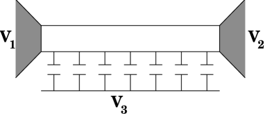
FIG. 5.: The 1D wire, connected to two reservoirs and coupled capacitively to a gate. After Ref. [37].

geometric capacitance of the wire to the gate per unit length, the Coulomb interaction adds an energy

$$\int dx\frac{e^{2}}{2c}\rho^{2}(x)$$ (25)

where $\rho$ is the excess density of electrons on the wire. Such a potential energy term is characteristic for Luttinger models for which the interaction term is written as $\nu^{-1}\int dx(1-1/g^{2})\rho^{2}(x)$ where $g$ is the interaction parameter and $\nu=1/hv$ the density of states at the Fermi energy. Here $v$ is the Fermi velocity. Comparison of the two terms gives a connection between the geometrical capacitance, the density of states and the interaction parameter, $g^{2}=1/(1+e^{2}\nu/c)$. As a consequence the electrochemical capacitance of the wire to the gate $c_{33}=c_{\mu}$ can be found by using Eq. (5) and per unit length can be written as[37]

$$c_{\mu}=g^{2}e^{2}\nu.$$ (26)

If the variation of the potential near the contacts is neglected the ground state can be taken to be uniform. The potential which develops if one of the contact voltages is varied is non-uniform and depends on the frequency. Nevertheless, Blanter et al. [37] find that a one-channel wire of length $L$, coupled capacitively to a gate, has a low frequency expansion of $G_{33}\equiv G(\omega)$ given by

$$G(\omega)=-i\omega C_{\mu}+\omega^{2}C_{\mu}^{2}R_{q}+O(\omega^{3})$$ (27)

with $C_{\mu}=Lc_{\mu}$ and a charge relaxation resistance given by

$$R_{q}=h/4e^{2}.$$ (28)

Note again that the charge relaxation resistance corresponds to the parallel addition of two conductances (one per contact) of $2e^{2}/h$. It is shown in Ref. [37] that a measurement of $G_{33}\equiv G(\omega)$ up to the third order in frequency permits to determine the interaction constant $g$.

The quantization of the charge relaxation resistance is lost as soon as we consider a many channel ballistic wire. If the velocity of channel $i$ at the Fermi energy is $v_{i}$ the charge relaxation resistance of an N channel ballistic wire is given by[38, 39]

$$R_{q}=\frac{h}{4e^{2}}\frac{\sum_{i=1}^{i=N}(\frac{1}{hv_{i}})^{2}}{[\sum_{i=1}^{i=N}\frac{1}{hv_{i}}]^{2}}$$ (29)

This resistance varies between $R_{q}=h/4e^{2}N$ when all density of states are comparable and $R_{q}=h/4e^{2}$ when one of the density of states is very much larger than all others.

In a two dimensional electron gas in a high magnetic field the extended states at the Fermi surface which give rise to the quantized Hall resistance are edge states. For each Landau level that is below the Fermi energy in the bulk of a Hall bar there exists an edge state with velocity $v^{u}_{i}$ at the upper edge and with velocity $v^{l}_{i}$ at the lower edge. In reality the edge state follows an equipotential line and the velocity is thus space dependent. We need the density of states $1/hv$ rather than the velocities themselves. To take the spatial variation into account we can introduce the density of states averaged along an edge state over the entire length of the Hall bar. Furthermore, the electrostatic potential can differ for different edge states on the same edge of the sample. Here we assume for simplicity that all edge states of the sample are at the same potential $U^{u}$ at the upper edge and at the same potential $U^{l}$ at the lower edge. A dipole is established in this sample by charging the upper edge states against the edge states on the lower edge. The relaxation of the excess charge on the edge states is then determined by a charge relaxation resistance which according to Christen and the author[40] is given by

$$R_{q}=\frac{h}{2e^{2}}\left(\frac{\sum_{i=1}^{i=N}(\frac{1}{hv^{u}_{i}})^{2}}{[\sum_{i=1}^{i=N}\frac{1}{hv^{u}_{i}}]^{2}}+\frac{\sum_{i=1}^{i=N}(\frac{1}{hv^{l}_{i}})^{2}}{[\sum_{i=1}^{i=N}\frac{1}{hv^{l}_{i}}]^{2}}\right).$$ (30)

Like the charge relaxation resistance of a ballistic wire, it is dominated by the channel with the highest density of states (smallest Fermi velocity). Here we can imagine that the upper edge presents a much smoother potential then the lower edge. In that case the charge relaxation resistance might be as high as $R_{q}=h/2e^{2}$.

D Charge Relaxation Resistance of a Quantum Point Contact

A quantum point contact is a constriction in a two dimensional electron gas with a lateral width of the order of a Fermi wavelength [41, 42] . We combine the capacitances of the conduction channel to the two gates and describe the interaction of the quantum point contact with the gates with the help of a single geometrical capacitance $C$. A simple model of a quantum point contact takes the potential to be a saddle point at the center of the constriction[43, 44],

$$V(x,y)=V_{0}+\frac{1}{2}m\omega_{y}^{2}y^{2}-\frac{1}{2}m\omega_{x}^{2}x^{2}$$ (31)

where $V_{0}$ is the electrostatic potential at the saddle and the curvatures of the potential are parametrized by $\omega_{x}$ and $\omega_{y}$. For this model the scattering matrix is diagonal, i.e. for each quantum channel ( energy $\hbar\omega_{y}(n+1/2)$ for transverse motion) it can be represented as a $2\times 2$-matrix. For a symmetric scattering potential and without a magnetic field the scattering matrix is of the form

$$s_{n}(E)=\left(\begin{array}[]{ll}-i\sqrt{R_{n}}\exp(i\phi_{n})&\sqrt{T_{n}}\exp(i\phi_{n})\\ \sqrt{T_{n}}\exp(i\phi_{n})&-i\sqrt{R_{n}}\exp(i\phi_{n})\end{array}\right)$$ (32)

where $T_{n}$ and $R_{n}=1-T_{n}$ are the transmission and reflection probabilities of the n-th quantum channel and $\phi_{n}$ is the phase accumulated by a carrier in the n-th channel during transmission through the QPC. The probabilities for transmission through the saddle point are[43]

$$T_{n}(E) = \frac{1}{1+e^{-\pi\epsilon_{n}(E)}},$$ (33)

$$\epsilon_{n}(E) = 2\left[E-\hbar\omega_{y}(n+\frac{1}{2})-V_{0}\right]/(\hbar\omega_{x}).$$ (34)

The transmission probabilities determine the conductance $G=({e^{2}}/{h})\sum_{n}T_{n}$ and the zero-frequency shot-noise [36, 45, 46, 47] $S(\omega=0,V)=({e^{2}}/{h})(\sum_{n}T_{n}R_{n})e|V|$. As a function of energy (gate voltage) the conductance rises step-like[41, 42]. The shot noise is a periodic function of energy. The oscillations in the shot noise associated with the opening of a quantum channel have recently been demonstrated experimentally in a clear and unam-

FIG. 6.: Density of states in units of $4/(h\omega_{x})$ for a saddle-point constriction as function of energy, $E/(\hbar\omega_{x})$. After Ref. [32].

biguous manner by Reznikov et al.[48] and Kumar et al.[49]. Deviations from the equilibrium charge distribution can occur in various ways[3, 2]. If the capacitances to the gate are large the charge distribution takes the form of a dipole[3, 9] across the QPC. If the geometrical capacitance for this dipole is large the QPC can be charged vis-a-vis the gate[2]. Here we consider the latter situation.

First we now need the density of states of the QPC. To this end we use the relation between density and phase $D_{n}=(1/\pi)\phi_{n}$ and evaluate it semi-classically. The spatial region of interest for which we have to find the density of states is the region over which the electron density in the contact is not screened completely. We denote this length by $\lambda$. The density of states is then found from $N_{n}=1/h\int_{-\lambda}^{\lambda}\frac{dp_{n}}{dE}dx$ where $p_{n}$ is the classically allowed momentum. A simple calculation gives a density of states

$${\cal D}_{n}(E)=\frac{4}{h\omega_{x}}\mbox{asinh}\left(\sqrt{\frac{1}{2}\frac{m\omega_{x}^{2}}{E-E_{n}}}\lambda\right),$$ (35)

for energies $E$ exceeding the channel threshold $E_{n}$ and

$${\cal D}_{n}(E)=\frac{4}{h\omega_{x}}\mbox{acosh}\left(\sqrt{\frac{1}{2}\frac{m\omega_{x}^{2}}{E_{n}-E}}\lambda\right),$$ (36)

for energies in the interval $E_{n}-(1/2)m\omega_{x}^{2}\lambda^{2}\leq E<E_{n}$ below the channel threshold. Electrons with energies less than $E_{n}-\frac{1}{2}m\omega_{x}^{2}\lambda^{2}$ are reflected before reaching the region of interest, and thus do not contribute to the density of states. The resulting density of states has a logarithmic singularity at the threshold $E_{n}=\hbar\omega_{y}(n+\frac{1}{2})+V_{0}$ of the n-th quantum channel. (We expect that a fully quantum mechanical calculation gives a density of states which exhibits also a peak at the threshold but which is not singular). The total density of states ${\cal D}=\sum_{n}{\cal D}_{n}$ as function of energy (gate voltage) is shown in Fig. 6 for $\omega_{y}/\omega_{x}=3$, $V_{0}=0$ and $m\omega_{x}\lambda^{2}/\hbar=18$. Each peak in the density of states of Fig. 6 marks the opening of a new channel. With the help of the density of states we also obtain the capacitance $C_{\mu}^{-1}=C^{-1}+(e^{2}{\cal D})^{-1}$.

It is instructive to evaluate the resistances $R_{q}$ explicitly in terms of the parameters which determine the scattering matrix. We find for the density of states matrix of the n-th quantum channel,

FIG. 7.: Effective resistance, in units of $h/e^{2}$, as function of energy, $E/(\hbar\omega_{x})$ for the cases $a)\hskip 4.26773pt\hbar\omega/(eV)=0$, $b)\hskip 4.26773pt\hbar\omega/(eV)=0.25$, $c)\hskip 4.26773pt\hbar\omega/(eV)=0.5$ and $d)\hskip 4.26773pt\hbar\omega/(eV)=1$, where $V$ is the bias voltage. After Ref. [32].

$${\cal N}_{11} = {\cal N}_{22}=\frac{1}{2\pi}\frac{d\phi_{n}}{dE},$$ (37)

$${\cal N}_{12} = {\cal N}_{21}=\frac{1}{4\pi}\frac{1}{\sqrt{R_{n}T_{n}}}\frac{dT_{n}}{dE}.$$ (38)

Inserting these results into the expression for the charge relaxation resistance Eq. (6) gives curve (d) in Fig. 7.

The resistance $R_{v}$ is given by [32]

$$R_{v} = \frac{h}{e^{2}}\frac{\sum_{n}\frac{1}{4R_{n}T_{n}}\left(\frac{dT_{n}}{dE}\right)^{2}}{[\sum_{n}(d\phi_{n}/dE)]^{2}}.$$ (39)

It is sensitive to the variation with energy of the transmission probability. Note that the transmission probability has the form of a Fermi function. Consequently, the derivative of the transmission probability is also proportional to $T_{n}R_{n}$. The numerator of Eq. (39) is thus also maximal at the onset of a new channel and vanishes on a conductance plateau.

In Fig. 7 the effective resistance $R(\omega,V)$ is shown for four frequencies $\hbar\omega/(eV)=0,0.25,0.5,1$, where $V$ is the applied voltage. At the highest frequency $\hbar\omega/(eV)=1$ the resistance $R(\omega,V)$ is completely dominated by the equilibrium charge relaxation resistance $R_{q}$. The uppermost curve (d) of Fig. 7 is nothing but $R_{q}$ and determines the noise due to the zero-point equilibrium fluctuations. The fluctuations reach a maximum at the onset of a new channel since $R_{q}$ takes its maximum value, $R_{q}=h/e^{2}$. At the lowest frequency $\hbar\omega=0$ the resistance $R(\omega,V)$ is determined by $R_{v}$. The lowermost curve (a) of Fig. 7 is the nonequilibrium resistance $R_{v}$. It is seen that the non-equilibrium resistance $R_{v}$ is very much smaller than $R_{q}$. We have encountered such a difference between $R_{q}$ and $R_{v}$ already for the chaotic cavities. Furthermore $R_{v}$ exhibits a double peak structure: The large peak in the density of states at the threshold of a quantum channel nearly suppresses the non-equilibrium noise at the channel threshold completely. Two additional curves (b and c for $\hbar\omega/(eV)=0.25$ and $\hbar\omega/(eV)=0.5$) describe the crossover from $R_{v}$ to $R_{q}$.

The resistances $R_{q}$ and $R_{v}$ probe an aspect of mesoscopic conductors which is not accessible by investigating the dc-conductance or the zero-frequency limit of shot noise. A more realistic treatment of the charge distribution of a quantum point contact includes a dipole across the quantum point contact itself[3, 9] and in the presence of the gates includes a quadrupolar charge distribution[2].

V Discussion

In this work we have summarized our current understanding of the relaxation of excess charge and its fluctuations both at equilibrium and in a transport state of mesoscopic conductors. At low frequencies the dynamics of the charge is governed by an out-of-phase response which is given by an electrochemical capacitance or a kinetic inductance. The dissipative, in-phase response is determined by a charge relaxation resistance. For the simple models investigated here, we find that the charge relaxation resistance is universal in the single channel limit and in the two channel limit is universal for systems with a uniform ground state (ballistic wire). In general, for systems connected to two or more channels the charge relaxation resistance is sample specific. For the case of chaotic cavities connected to two channels we have discussed the distribution of the charge relaxation resistances. For cavities connected to many channels the average charge relaxation resistance has a classical part and a quantum mechanical weak localization correction. We have also discussed the charge relaxation resistance for systems subject to quantizing magnetic fields and found that it is dominated by the edge channel with the highest density of states. For a quantum point contact we have found that the charge relaxation resistance peaks at the opening of a new channel.

While we have discussed charge relaxation resistances for a number of different conductors, there are still a number of important cases which we have not treated. For instance, the charge relaxation resistance of a metallic diffusive mesoscopic wire is not known [50]. For a metallic wire close to a gate, we expect that a small variation of the gate voltage changes the potential only near the surface of the metallic wire within a depth of a screening length. Thus the charge relaxation resistance can be expected to be determined by the time it takes the excess charge which resides in this screening layer to move in and out of the conductor. The considerations presented above for the quantized Hall conductors should be extended to the case where we are in between plateaus and the bulk states becomes important. This problem thus requires also an understanding of charge relaxation in insulators.

We have also investigated the fluctuations of the charge. At equilibrium these fluctuations are governed by the charge relaxation resistance. The charge fluctuations in a transport state are governed by a non-equilibrium charge relaxation resistance. We expect that the internal potential fluctuations are important for the discussion of dephasing in small conductors.

The charge relaxation of mesoscopic conductors is clearly a very interesting subject with so far little theoretical and experimental interest. We hope that this work stimulates a wider interest for the charge dynamics of mesoscopic conductors.

REFERENCES

- [1] M. Büttiker, H. Thomas, and A. Prêtre, Phys. Lett. A 180, 364 (1993).
- [2] M. Büttiker and T. Christen, in Mesoscopic Electron Transport, ed. by L. P. Kouwenhoven, G. Schön, and L. L. Sohn, NATO ASI Series E (Kluwer Academic Publishing, Dordrecht, 1997). Vol. 345. p. 259.
- [3] T. Christen and M. Büttiker, Phys. Rev. Lett. 77, 143 (1996).
- [4] T. Christen and M. Büttiker, Europhys. Lett. 35, 523 (1996).
- [5] A. M. Song, A. Lorke, A. Kriele, J. P. Kotthaus, W. Wegschneider, M. Bichler, Phys. Rev. Lett. 80, 3831 (1998).
- [6] Z. S. Ma, J. Wang, and H. Guo, Phys. Rev. B 57, 9108 (1998).
- [7] V. A. Sablikov and B. S. Shschamkhalova, Phys. Rev. 58, 13847 (1998).
- [8] M. P. Anatram, J. Phys. Cond. Mat. 10, 9015 (1998).
- [9] I. E. Aronov, et al. Phys. Rev. B 58, 9894 (1998).
- [10] S. Kurokawa and A. Sakai, J. of Applied Physics, 83, 7416 (1998).
- [11] M. H. Pedersen and M. Büttiker, Phys. Rev. B 58, 12993 (1998).
- [12] R. Aguado and G. Platero, Phys. Rev. Lett. 81 4971 (1998).
- [13] C. S. Tang and C. S. Chu, (unpublished).
- [14] F. T. Smith, Phys. Rev. 118 349 (1960).
- [15] It is the derivative with respect to the potential and not the energy which are fundamental. The phase derivatives with respect to the potential lead to a dwell time which differs from the Wigner-Smith phase-delay times, M. Büttiker, Phys. Rev. B 27, 6178 (1983) and C. R. Leavens and G. C. Aers, Phys. Rev. B39, 1202 (1989).
- [16] M. Büttiker, in ”Electronic Properties of Multilayers and low Dimensional Semiconductors”, edited by J. M. Chamberlain, L. Eaves, and J. C. Portal, (Plenum, New York, 1990). p. 297.
- [17] Y. Imry, in Directions in Condensed Matter Physics, edited by G. Grinstein and G. Mazenko, (World Scientific Singapore, 1986). p. 101.
- [18] R. Landauer, Z. Phys. B 68, 217 (1987).
- [19] M. Büttiker, Phys. Rev. Lett. 57, 1761 (1986); Phys. Rev. B 40, 3409 (1989).
- [20] T. Gramespacher and M. Büttiker, Phys. Rev. B 56, 13026 (1997).
- [21] F. Sols and J. Sanchez-Ca izares, cond-mat/9811325
- [22] M. Büttiker, J. Math. Phys., 37, 4793 (1996).
- [23] A. Kaminski, I. L. Aleiner, L. I. Glazman, Phys. Rev. Lett. 81, 685 (1998); I. L. Aleiner and L. I. Glazman, Phys. Rev. B 57, 9608 (1998).
- [24] C. M. Marcus, R. M. Westervelt, P. F. Hopkins and A. C. Gossard, Phys. Rev. B 48, 2460 (1993); M. Switkes, C. M. Marcus , K. Campman, A. C. Gossard, (unpublished).
- [25] C. W. J. Beenakker, Rev. Mod. Phys. 69, 731 (1997).
- [26] Y. V. Fyodorov and H. J. Sommers, Phys. Rev. Lett. 76, 4709 (1996).
- [27] V. A. Gopar, P. A. Mello, and M. Büttiker, Phys. Rev. Lett. 77, 3005 (1996).
- [28] V. A. Gopar and P. A. Mello, Europhys. Letters, 42, 131 (1998).
- [29] P. W. Brouwer, K. M. Frahm, and C. W. J. Beenakker, Phys. Rev. Lett. 78, 4737 (1997).
- [30] P. W. Brouwer, S. A. van Langen, K. M. Frahm, M. Büttiker and C. W. J. Beenakker, Phys. Rev. Lett. (1997).
- [31] S. F. Godijn, S. Moeller, H. Buhmann, L. W. Molenkamp, S. A. van Langen, cond-mat/9811181.
- [32] M. H. Pedersen, S. A. van Langen, M. Büttiker, Phys. Rev. B 57, 1838 (1998).
- [33] P. Sebbah, O. Legrand, A. Z. Genack,cond-mat/9808237 .
- [34] P. W. Brouwer and C. W. J. Beenakker, J. Math. Phys. 37, 4904 (1996).
- [35] P. W. Brouwer and M. Büttiker, Europhys. Lett. 37, 441 (1997).
- [36] M. Büttiker, Phys. Rev. Lett. 65, 2910 (1990); Phys. Rev. B 46, 12485 (1992).
- [37] Ya. M. Blanter, F.W.J. Hekking, and M. Büttiker, Phys. Rev. Lett. 81, 1749 (1998).
- [38] M. Büttiker and T. Christen, in Quantum Transport in Semiconductor Submicron Structures, edited by B. Kramer, (Kluwer Academic Publishers, Dordrecht, 1996); NATO ASI Series, Vol. 326, 263 (1996).
- [39] Y. M. Blanter and M. Büttiker, Europhys. Lett. 42 535 (1998).
- [40] M. Büttiker and T. Christen, in ’High Magnetic Fields in the Physics of Semiconductors’, edited by G. Landwehr and W. Ossau, (World Scientific, Singapur, 1997). p. 193.
- [41] B. J. van Wees, H. van Houten, C. W. J. Beenakker, J. G. Williamson, L. P. Kouwenhoven, D. van der Marel and C. T. Foxon, Phys. Rev. Lett. 60, 848 (1988).
- [42] D. A. Wharam, T. J. Thornton, R. Newbury, M. Pepper, H. Ahmed, J. E. F. Frost, D. G. Hasko, D. C. Peacock, D. A. Ritchie and G. A. C. Jones, J. Phys. C 21, L209 (1988).
- [43] M. Büttiker, Phys. Rev. B 41, 7906 (1990).
- [44] A. G. Scherbakov, E. N. Bogachek, and U. Landman, Phys. Rev. B 53, 4054 (1996).
- [45] G. B. Lesovik, Pisma Zh. Eksp. Teor. Fiz. 49, 513 (1989) (JETP Lett. 49, 592 (1989)).
- [46] M. Büttiker, Physica B 175, 199 (1991).
- [47] Th. Martin and R. Landauer, Phys. Rev. B 45, 1742 (1992).
- [48] M. Reznikov, M. Heiblum, H. Shtrikman, and D. Mahalu, Phys. Rev. Lett. 75, 3340 (1995).
- [49] A. Kumar, L. Saminadayar, D. C. Glattli, Y. Jin, and B. Etienne, Phys. Rev. Lett. 76, 2778 (1996).
- [50] For one-dimensional motion in random potentials the distribution of the global phase-delay is knwon: See C. Texier and A. Comtet, cond-mat/9812196 and J. Phys. A: Math. Gen. 36, 8017 (1997); S. K. Joshi and and A. M. Jayannavar, cond-mat/9712249; A. M. Jayannavar, C. V. Vijayagovindan and N. Kumar, Z. Phys. B 75, 77 (1989).