Density Matrix Renormalization Group and Reaction-Diffusion Processes

Abstract

The density matrix renormalization group (dmrg) is applied to some one-dimensional reaction-diffusion models in the vicinity of and at their critical point. The stochastic time evolution for these models is given in terms of a non-symmetric “quantum Hamiltonian”, which is diagonalized using the dmrg method for open chains of moderate lengths (up to about $60$ sites). The numerical diagonalization methods for non-symmetric matrices are reviewed. Different choices for an appropriate density matrix in the non-symmetric dmrg are discussed. Accurate estimates of the steady-state critical points and exponents can then be found from finite-size scaling through standard finite-lattice extrapolation methods. This is exemplified by studying the leading relaxation time and the density profiles of diffusion-annihilation and of a branching-fusing model in the directed percolation universality class.

1 Introduction

The density matrix renormalisation group (dmrg) technique was invented by White Whit92 in 1992 as a new tool for the diagonalization of quantum chain spin Hamiltonians. The dmrg allows to study much larger systems than is possible with standard exact diagonalization methods and provides data with remarkable accuracy. The method has since been applied to a large variety of systems in quantum quantum and classical classical physics. These applications usually considered hermitian quantum Hamiltonians for spin chains or symmetric transfer matrices for two-dimensional classical systems. In both cases the dmrg is known to work very well. For a collection of reviews see DMRGBook .

Motivated by the success obtained for these problems, some efforts have been recently devoted to problems involving diagonalization of non-symmetric matrices which are often encountered in various fields of physics; as example we mention the cases of low temperature thermodynamics of spin chains bursill or out-of-equilibrium classical systems hieda ; kaulke .

The models investigated in this paper belong to the latter class of problems. We consider one-dimensional reaction-diffusion systems where the stochastic time evolution of the system is given by a non-hermitean operator $H$ to which we apply the dmrg algorithm. One of the models considered displays a non-equilibrium phase transition which is expected to be in the universality class of directed percolation, a typical class for many out-of-equilibrium systems and for which the critical exponents are known numerically to a high degree of accuracy.

Our main motivation for this study is as follows. At equilibrium, studies of finite systems through diagonalization of a transfer matrix and/or a quantum Hamiltonian and analysis of the results through finite-size scaling, eventually combined with precise extrapolation algorithms, has been one of the standard methods of studying phase transitions in systems with many strongly interacting degrees of freedom Priv90 ; Card88 ; Henk99 . Compared to more standard diagonalization methods, the dmrg does allow to study much larger systems, even if it works best in situations when the ground state of $H$ is separated by a finite gap from the first excited state, that is, at a finite distance away from the critical point. That advantage is at least partially offset by the fact that for reasons of numerical accuracy, it is preferable to apply the dmrg to models with open boundary conditions, which lead to estimates of the critical parameters which converge usually slower than those found for periodic boundary conditions. Here we study to what extent a finite-size diagonalization study of non-equilibrium systems is feasible and in particular, to what degree of precision critical points and critical exponents can be estimated. For that purpose, we shall consider some critical non-equilibrium models with known properties to compare with our dmrg data.

Diagonalizing non-symmetric matrices is numerically much more demanding than for symmetric matrices. Potentially, numerical instabilities might arise at several stages of the calculation. We shall discuss in some detail various diagonalization methods for non-symmetric matrices and have tested our results throughout by working with two different diagonalization algorithms.

We shall not only consider the calculation of eigenvalues, which determine the relaxation times, but also of eigenvectors, which are needed in the calculation of matrix elements, as they arise for example in the calculation of density profiles. In general, we find that for non-symmetric matrices the numerical accuracy is not as good as for symmetric ones. However, we shall show that the dmrg is well capable to accurately determine the values of the critical parameters. This makes this technique a useful general-purpose method for the study of non-equilibrium critical phenomena.

This paper is organized as follows: in section 2, we introduce reaction-diffusion systems and their description in terms of non-symmetric evolution matrices, in section 3 we review the basics of the dmrg algorithm, and present in section 4 a brief review of diagonalization methods for non-symmetric matrices. More specific details about choosing a convenient density matrix for non-equilibrium systems are described in section 5. In sections 6 and 7 we present our numerical results concerning the critical properties of the model and then conclude.

2 Reaction-diffusion processes

We consider a chain of length $L$ in which each site is either occupied by a particle ($A$) or empty ($\emptyset$). The time evolution of the system is given in terms of microscopic rules involving only a pair of particles on neighbouring sites. We shall consider the following system, using the notation of Henk97 :

$$A\emptyset\leftrightarrow\emptyset A\,\,\,\,({\rm with}\,\,{\rm rate}\,\,D)$$ (1)

$$AA\rightarrow\emptyset\emptyset\,\,\,\,\,({\rm with}\,\,{\rm rate}\,\,2\alpha)$$ (2)

$$AA\rightarrow\emptyset A,A\emptyset\,\,\,\,\,({\rm with}\,\,{\rm rate}\,\,\gamma)$$ (3)

$$A\emptyset,\emptyset A\rightarrow\emptyset\emptyset\,\,\,\,\,({\rm with}\,\,{\rm rate}\,\,\delta)$$ (4)

$$A\emptyset,\emptyset A\rightarrow AA\,\,\,\,\,({\rm with}\,\,{\rm rate}\,\,\beta)$$ (5)

Apart from the diffusion process (1), all the other processes involve either a decrease (2,3,4) or an increase (5) in the number of particles (see Henk97 for a list of common alternative notations).

Once the reaction rates are given, the stochastic evolution follows from the master equation, which can be written as

$$\frac{d|P(t)\rangle}{dt}=-H|P(t)\rangle$$ (6)

where $|P(t)\rangle$ is the state vector. The elements of the quantum “Hamiltonian” $H$ are given by

$$\langle\sigma|H|\tau\rangle = -w(\tau\rightarrow\sigma)\;\;;\;\;\sigma\neq\tau$$

$$\langle\sigma|H|\sigma\rangle = \sum_{\tau\neq\sigma}w(\sigma\rightarrow\tau)$$ (7)

where $|\sigma\rangle$, $|\tau\rangle$ are the state vectors of the particle configurations $\sigma,\tau$ and $w(\tau\rightarrow\sigma)$ denotes the transition probability between the two states and is easily constructed from the rates (1-5) of the elementary processes. Since $H$ is a stochastic matrix, the left ground state $\langle s|$ is

$$\langle s|=\sum_{\sigma}\langle\sigma|$$ (8)

with ground state energy $E_{0}=0$, since $\langle s|H=0$. All other eigenvalues $E_{i}$ of $H$ have a non-negative real part $\Re E_{i}\geq 0$ Kamp81 . Since the formal solution of eq. (6) is

$$|P(t)\rangle=e^{-Ht}|P(0)\rangle$$ (9)

the system evolves towards its steady state $|P(\infty)\rangle$. Let $\Gamma:=\inf_{i}\Re E_{i}$ for $i\neq 0$. Often, one simply has

$$\Gamma=E_{1}-E_{0}=E_{1}$$ (10)

since $E_{0}=0$. If $\Gamma>0$, the approach towards the steady state is characterized by a finite relaxation time $\tau=1/\Gamma$, but if $\Gamma=0$, that approach is algebraic. This situation is quite analogous to non-critical phases ($\tau\neq 0$) and critical points ($\tau=0$), respectively, which may arise in equilibrium quantum Hamiltonians.

It is clear that $H$ is non-symmetric if $w(\sigma\rightarrow\tau)\neq w(\tau\rightarrow\sigma)$. However, if the detailed-balance condition

$$w(\sigma\rightarrow\tau)P_{s}(\{\tau\})=w(\tau\rightarrow\sigma)P_{s}(\{\sigma\})$$ (11)

is satisfied, where $P_{s}(\{\sigma\})$ is defined by $|P(\infty)\rangle=\sum_{\sigma}P_{s}(\{\sigma\})|\sigma\rangle$, $H$ is similar to a non-stochastic, but symmetric matrix $K$, without affecting the locality of the interactions, e.g. Kamp81 ; Ciep98 . Detailed balance always holds when besides diffusion only a single reversible reaction is present. For several reversible reactions, the cases when detailed balance holds are given in Alca94 , eq. (4.48). Only if detailed balance holds, the right ground state $|s\rangle=|P(\infty)\rangle$ is related to the known left ground state $\langle s|$ in a simple way fuss1 .

In this paper, we shall study systems without detailed balance, since it is our aim to explore the dmrg in a setting as different from equilibrium physics as possible. Specifically, we shall consider two models:

(1) Diffusion-annihilation. The rates are

$$D=2\alpha=p\;\;,\;\;\beta=\gamma=\delta=0$$ (12)

This model is characterized by an algebraic approach towards the steady state with a gap vanishing in the thermodynamic limit as $\Gamma\sim 1/L^{2}$. It offers to us the additional advantage that $H$ can be diagonalised through free-fermion methods (e.g. Alca94 ) and thus analytical results are available for comparison with the numerical data.

(2) Branching-fusing. Here we take

$$D=2\alpha=\gamma=\delta=1-p\;\;,\;\;\beta=p$$ (13)

This model presents a non-equilibrium phase transition. For $p$ small, the annihilating processes dominate and the steady state is simply the empty lattice. However, if $p$ becomes sufficiently large, the steady state contains particles at some finite density. The transition between these two phases is expected to fall into the directed percolation universality class (see also appendix A). Although even in $1D$, there is no analytical information available, series expansion studies and Monte Carlo simulation have over the years yielded extremely precise estimates of critical exponents, as reviewed in Essa96 and Muno98 ; Laur97 . We collect some of their results in table 1, but skip over repeating the precise exponent definitions here. We use the notation $\theta=\nu_{\|}/\nu_{\perp}$ for the dynamical exponent in order to avoid confusion with the exponent $z=2/\theta$ which is also often used. If $D=0$, the model would reduce to standard site-bond directed percolation, but the presence of $D$ should not change the universality class. The last column of table 1 shows the values of the exponents obtained from finite-size scaling extrapolation of our numerical data.

Table 1: Some critical exponents for $1D$ directed percolation, as obtained from series data Essa96 and Monte Carlo simulations Muno98 ; Laur97 . In the last column, the values obtained by density matrix renormalization in the present work are listed. The numbers in brackets give the estimated uncertainty.

exponent	series	simulation	this work
$\beta$	0.27647(10)	0.27649(4)
$\beta/\nu_{\perp}$	0.2520(1)	0.25208(4)	0.249(3)
$\beta_{1}$	0.7338(1)	0.728(1)
$\beta_{1}/\nu_{\perp}$	0.6690(1)	0.664(7)	0.667(2)
$\nu_{\|}$	1.7338(1)	1.73383(3)
$\nu_{\perp}$	1.0969(1)	1.09684(1)	1.08(2)
$\theta=\nu_{\|}/\nu_{\perp}$	1.5806(2)	1.58074(4)	1.580(1)

In both models (12,13), the empty lattice $|\emptyset\ldots\emptyset\rangle$ is obviously an adsorbing state and consequently also a steady state. Since $H$ is real, its eigenvalues are either real or occur in complex conjugate pairs. The first excited eigenvalue $E_{1}$ is always real.

For the branching-fusing model, we also considered the case of particle injection at the boundaries of the system, i.e. we added the reaction

$$\emptyset\rightarrow A\,\,\,\,\,({\rm with}\,\,{\rm rate}\,\,p^{\prime})$$ (14)

at the two sites at the edges. In this situation, $|\emptyset\ldots\emptyset\rangle$ is no longer a stationary state of the system since the lattice is occupied by a non-vanishing density of particles for all values of $p$. We analyze the shape of the density profiles as function of the parameter $p$ and of the injection rate $p^{\prime}$.

3 Density matrix renormalization group algorithm

We recall briefly in this section the basic structure of the dmrg algorithm Whit92 . The task is to find selected approximate eigenvalues and eigenvectors of a given Hamiltonian $H$. That desired eigenvector $|\psi\rangle$ is called a target state and the process of selecting $|\psi\rangle$ is referred to as targeting (it is possible to target several states, see below). One assumes that $H$ as defined on a open chain with $L$ sites and has the local structure

$$H=\sum_{i=1}^{L-1}h_{i,i+1}$$ (15)

where $h_{i,i+1}$ is a local Hamiltonian acting on a pair of nearest-neighbour sites (this condition of locality can be somewhat relaxed but we restrict here to the simplest case). In this paper, we always consider free (open) boundary conditions, as typically done in dmrg studies.

The dmrg is an iterative method: it produces a chosen eigenvector (usually, one targets the ground state or the first excited state) and its eigenvalue, starting from the target state of a small chain which is known from exact diagonalization of the Hamiltonian (15), and then using it to find $|\psi\rangle$ on chains with an increasing number of sites. This is made possible by projecting at each iteration step the full vector space to a smaller space where only a selected number $m$ of states is kept. This projection is carried out via the density matrix as described below.

A dmrg calculation, at least in the context of applications to critical phenomena, proceeds in two steps. The first one is the infinite system method (ism) which we now describe. Suppose we are interested in the ground state of $H$. As the starting point, consider a chain of four lattice sites which can be represented as $B_{l}^{(1)}\bullet\bullet B_{r}^{(1)}$, where $\bullet$ denotes a single site and $B_{r,l}^{(1)}$ are blocks at the left and right side of the chain. Initially, they contain only one spin, that is $B_{r,l}^{(1)}=\bullet$ (of course, the calculation may be started at larger lattices)

At this point, the main loop begins. The Hamiltonian $H$ is easily written down and its ground state wave function $\psi_{0}(\alpha_{l},i_{l},j_{r},\beta_{r})$ can be found via standard diagonalization routines, where $\alpha_{l}$ and $\beta_{r}$ denote degrees of freedom of the blocks $B_{r}^{(1)}$ and $B_{l}^{(1)}$ and the indices $i_{l},j_{r}$ refer to the spin degrees of freedom of the single lattice points in the middle of the chain. The density matrix for the left part of the system is defined as

$$\rho^{(l)}(\alpha_{l},i_{l};\gamma_{l},k_{l})=\sum_{j_{r},\beta_{r}}\psi_{0}(\alpha_{l},i_{l},j_{r},\beta_{r})\psi_{0}(\gamma_{l},k_{l},j_{r},\beta_{r})$$ (16)

which we shall write in a short-hand notation as $\rho=\widehat{\mbox{\rm tr\,}}(|\psi_{0}\rangle\langle\psi_{0}|)$, where $\widehat{\mbox{\rm tr\,}}$ denotes a partial trace either in the left or right part of the system (we shall reconsider the precise choice of $\rho$ in section 5). Next, one solves the eigenvalue problem $\rho|\Omega_{i}\rangle=\omega_{i}|\Omega_{i}\rangle$. The eigenvalues of the density matrix are non-negative and can be ordered according to $\omega_{1}\geq\omega_{2}\geq\omega_{3}\geq\ldots\geq 0$. Furthermore, if the ground state vector of $H$ is normalized according to $\langle\psi_{0}|\psi_{0}\rangle=1$, one has $\sum_{i}\omega_{i}=1$. Each eigenvalue $\omega_{i}$ is equal to the probability of finding the left part of the chain in the corresponding density matrix eigenvector $|\Omega_{i}\rangle$ when the whole system is in the ground state $|\psi_{0}\rangle$. The configurational space reduction is obtained by keeping only the first $m$ dominant density matrix eigenvectors $|\Omega_{i}\rangle$ with $i=1,2,\ldots m$, corresponding to the $m$ largest $\omega_{i}$. Formally, the truncation can be represented by

$$O_{m}^{T}\left(B_{l}^{(1)}\bullet\right)O_{m}=B_{l}^{(2)}$$ (17)

where $O_{m}=[|\Omega_{1}\rangle,\ldots,|\Omega_{m}\rangle]$. The accuracy of the projection operation can be described by the truncation error:

$$\epsilon=1-\sum_{i=1}^{m}\omega_{i}$$ (18)

The projection operation is repeated for the right part as well to obtain $B_{r}^{(2)}$ (if there is a left-right symmetry, as in the models studied here, $B_{r}^{(2)}$ is obtained simply from reflection of $B_{l}^{(2)}$). Performing these calculations, sparse-matrix diagonalization techniques will be needed to obtain the ground eigenstate $|\psi_{0}\rangle$ of $H$. On the other hand, since the whole spectrum of the non-sparse matrix $\rho$ is required, this is best obtained via some standard routines.

Combining the two blocks with new sites one gets $B_{l}^{(2)}\bullet\bullet B_{r}^{(2)}$, e.g. a chain of $L=6$ sites after the first pass through the main loop. The next pass through the main loop begins by writing down $H$ for this longer chain.

Applying this procedure repeatedly at the left and right part of the system, one generates larger systems. At each iteration step, two new sites are added in the middle of the chain and the boundaries are pushed further away from each other. Schematically, this may be illustrated as

$$B_{l}^{(1)}\bullet\bullet B_{r}^{(1)}\rightarrow B_{l}^{(2)}\bullet\bullet B_{r}^{(2)}\rightarrow\ldots\rightarrow B_{l}^{(L/2-1)}\bullet\bullet B_{r}^{(L/2-1)}$$

The ism procedure is repeated, typically until $L\approx 1000$, and if there is a finite gap in the low-lying spectrum of $H$, finite-size effects can then be neglected. However, it is well known that the ism method alone is not enough to yield precise results in the thermodynamic limit $L\to\infty$ for systems close to criticality ostlund ; DMRGBook .

In such cases (e.g. ferenc ), a second step in the dmrg calculation is required. It is best to use the finite system method (fsm) designed by White Whit92 to accurately determine properties of systems of finite length. The starting point of the fsm is the target vector $|\psi\rangle$ for a chain of given length $L$, as generated by the ism described above. At this point further iterations are started. First, one calculates better approximations for the blocks on the left part representing more than $L/2-1$ sites, using as before eq. (17), while for the blocks on the right part, one uses blocks generated in previous iterations in order to keep the total length of the system fixed at $L$. Schematically this looks as follows

$$B_{l}^{(L/2-1)}\bullet\bullet B_{r}^{(L/2-1)}\rightarrow B_{l}^{(L/2)}\bullet\bullet B_{r}^{(L/2-2)}\rightarrow$$

$$\ldots\rightarrow B_{l}^{(L-3)}\bullet\bullet B_{r}^{(1)}$$

Second, this procedure is reversed and the larger blocks on right part of the system are refined. Schematically,

$$B_{l}^{(L-3)}\bullet\bullet B_{r}^{(1)}\rightarrow B_{l}^{(L-2)}\bullet\bullet B_{r}^{(2)}\rightarrow\ldots\rightarrow B_{l}^{(1)}\bullet\bullet B_{r}^{(L-3)}$$

In these steps, on the $B_{r}$ are updated according to eq. (17), while the $B_{l}$ are taken from the blocks calculated previously. Finally, the $B_{l}$ are updated again through the sequence

$$B_{l}^{(1)}\bullet\bullet B_{r}^{(L-3)}\rightarrow B_{l}^{(2)}\bullet\bullet B_{r}^{(L-4)}\rightarrow$$

$$\ldots\rightarrow B_{l}^{(L/2-1)}\bullet\bullet B_{r}^{(L/2-1)}$$

until one is back at the left-right symmetric partition. The target vector extracted at this stage can be used as starting point for the next fsm iteration.

These “sweeps” improve the results both for eigenvalues and eigenvectors Whit92 . For a given lattice size, two or three sweeps are usually enough to achieve convergence.

In practice, to calculate critical exponents, one needs data for chains of various lengths in order to perform a finite-size scaling analysis. For better efficiency, we used repeatedly the fsm to calculate from the same run quantities for chains of different lengths as follows. The blocks generated at the end of the fsm for a chain of length $L_{0}$ are used as starting point for further dmrg calculation: first, we use the ism to enlarge the system is symmetrically until a length $L_{1}>L_{0}$ is reached. Second, the fsm sweeps are started again. In this way we produced accurate results for systems of various lengths $L_{0}\leq L_{1}\leq\ldots$, typically equally spaced, in the same dmrg run.

4 Diagonalization methods for non-symmetric matrices

In “conventional” dmrg calculations the computationally dominant part is the determination of (ground state) wave functions given by the eigenvectors of a large sparse symmetric $N\times N$ matrix $A$ using a diagonalization algorithm for large sparse symmetric matrices such as the Lanczos algorithm. Using the fundamental operation

$$|w\rangle=A|v\rangle,$$ (19)

one builds iteratively small tridiagonal $n\times n$ matrices $T_{n}=Q^{T}_{n}AQ_{n}$ with $n\ll N$, where $Q_{n}$ is a $N\times n$ matrix with orthonormal columns. The matrices $T_{n}$ are diagonalisable by standard techniques; it can be shown that their extreme eigenvalues converge for rather small $n$ to the extreme eigenvalues of $A$. Moreover, their eigenvalues form Sturm chains: if $\lambda_{i}$ are the eigenvalues of $T_{n}$ in ascending order and $\mu_{i}$ those of $T_{n+1}$, one has $\mu_{i}<\lambda_{i}<\mu_{i+1}$. This ensures monotonous, easily controlled convergence of the extreme eigenvalues. $Q_{n}$ relates the eigenvectors of $T_{n}$ to those of $A$: $|\lambda_{0}\rangle_{A}=Q_{n}|\lambda_{0}\rangle_{T_{n}}$. In the case of large sparse non-symmetric matrices, as they arise in transfer matrix dmrg and non-hermitian dmrg, the situation is much less satisfying, as the lack of symmetry leads to intrinsic problems of numerical stability.

Essentially, there are two algorithms available, the Arnoldi algorithm and the non-symmetric Lanczos algorithm Golub . In our calculations, we used both methods, to check them against each other to guard against numerical fallacies. Usually, they were in excellent agreement, though the professional package available for the Arnoldi algorithm ARPACK usually seemed to be somewhat more accurate than our self-made implementation of the non-symmetric Lanczos algorithm.

Both also build on the fundamental operation

$$|w\rangle=A|v\rangle$$ (20)

and its transpose

$$\langle w|=\langle v|A$$ (21)

in the case of the non-symmetric Lanczos algorithm. Again, one builds iteratively small $n\times n$ matrices with $n\ll N$ diagonisable by standard techniques for small non-symmetric matrices. In both cases, one finds that the extreme eigenvalues of the small matrices do not converge to those of the big matrices in the very systematic manner of the symmetric case, i.e. they do not form Sturm chains.

The Arnoldi method iteratively generates one sequence of orthonormal vectors $|q_{i}\rangle$ forming the columns of a matrix $Q_{n}=[|q_{1}\rangle,\ldots,|q_{n}\rangle]$ and a Hessenberg matrix $H_{n}=Q^{T}_{n}AQ_{n}$ with elements $h_{ij}$. One starts from a random vector $|q_{0}\rangle$ of unit length and $h_{10}=1$ and iterates using

$$h_{k+1,k}|q_{k+1}\rangle=A|q_{k}\rangle-\sum_{i=1}^{k}h_{ik}|q_{i}\rangle$$ (22)

with $h_{ij}=\langle q_{i}|A|q_{j}\rangle$. $h_{k+1,k}$ is determined by enforcing unit length for $|q_{k+1}\rangle$. Here, $\langle q_{i}|=|q_{i}\rangle^{T}$.

The non-symmetric Hessenberg matrix is then diagonalized using the standard QR algorithm. Some of the eigenvalues of $H_{n}$ will converge against some of those of $A$, and associated eigenvectors of $H_{n}$ can be transformed into those of $A$ using $Q_{n}$. However, it is quite intricate to assure that eigenvalue convergence actually happens numerically. We will not discuss this issue further, as there is a freely available highly sophisticated Arnoldi package (arpack)ARPACK .

Let us now discuss the non-symmetric Lanczos algorithm, which is quite easily implemented, but has to be carefully refined for numerical stability. Then it provides a highly satisfying alternative approach portable to machines where arpack might not be available.

Let us first summarize the algorithm as presented in Ref. Golub . The non-symmetric Lanczos algorithm generates iteratively two sequences of vectors from whom eventually left and right eigenvectors are built. In an adaptation of the symmetric case, one forms matrices from these vectors, $Q_{n}=[|q_{1}\rangle,\ldots,|q_{n}\rangle]$ and $P_{n}=[\langle p_{1}|,\ldots,\langle p_{n}|]$, to generate an (incomplete) basis transformation from the $N\times N$ matrix $A$ to a tridiagonal $n\times n$ matrix $T_{n}$,

$$T_{n}=P_{n}AQ_{n}=\left[\begin{array}[]{ccccc}\alpha_{1}&\gamma_{1}&.&.&0\\ \beta_{1}&\alpha_{2}&\gamma_{2}&.&.\\ .&.&.&.&.\\ .&.&.&.&\gamma_{n-1}\\ 0&.&.&\beta_{n-1}&\alpha_{n}\end{array}\right]$$ (23)

and demands biorthogonality, $P_{n}Q_{n}=I_{n}$. One then obtains the following equations determining the elements of the tridiagonal matrix:

$$\beta_{k}|q_{k+1}\rangle := |t_{k}\rangle=(A-\alpha_{k}I)|q_{k}\rangle-\gamma_{k-1}|q_{k-1}\rangle$$ (24)

$$\gamma_{k}\langle p_{k+1}| := \langle s_{k}|=\langle p_{k}|(A-\alpha_{k}I)-\beta_{k-1}\langle p_{k-1}|$$ (25)

with

$$\alpha_{k} = \langle p_{k}|A|q_{k}\rangle$$ (26)

$$\beta_{k} = ||\,|t_{k}\rangle||$$ (27)

$$\gamma_{k} = \langle s_{k}|t_{k}\rangle/\beta_{k}.$$ (28)

Note that the choice of the off-diagonal coefficients is not unique. One starts with $|q_{0}\rangle=0$ and $\langle p_{0}|=0$ and two non-orthogonal random vectors $|q_{1}\rangle$ and $\langle p_{1}|$, normed such that $|q_{1}\rangle$ has unit length and $\langle p_{1}|q_{1}\rangle=1$ as input for the first iteration. This leads to an iteratively growing $T_{n}$. The iterations are continued, until the lowest (two) eigenvalues of $T_{n}$ are sufficiently converged. From the left and right eigenvectors of $T_{n}$ one forms the left and right eigenvectors of $A$: $|\lambda\rangle_{A}=Q_{n}|\lambda\rangle_{T_{n}}$ and $\langle\lambda|_{A}=\langle\lambda|_{T_{n}}P_{n}$.

Note that the non-symmetric Lanczos algorithm yields left and right eigenvectors on an equal footing, while the Arnoldi algorithm has to be run twice for $A$ and $A^{T}$ (however, with less time-consuming matrix-vector multiplications).

In the present form, the non-symmetric Lanczos algorithm is capable of yielding rather good eigenvalues. However, eigenvectors are determined with rather poor accuracy only. This leads to a poor choice for the density matrix, in turn to a non-optimized decimation and then, after some dmrg steps, to a noticeable degradation of the eigenvalues too. There are two reasons for this.

(1) The construction of the two Lanczos vector sequences guarantees them to be biorthogonal, or $\langle p_{i}|q_{j}\rangle=\delta_{ij}$. While true mathematically, this biorthogonality is numerically only true locally, i.e. if $i$ and $j$ are close. Globally, small overlaps develop, in particular when the extreme eigenvalues of $T_{n}$ start to converge. This loss of orthogonality introduces numerical errors in the mapping from the eigenvectors of $T_{n}$ to those of $A$. An analogous loss of orthogonality occurs in the Arnoldi algorithm.

(2) Even the symmetric Lanczos algorithm shows the phenomenon that if one wants a non-extreme, say the second, eigenvalue to converge, it may occur that the eigenvalue converges to its true value, but if one enforces too strict convergence criteria, “jumps” and will converge to the lowest eigenvalue, too, see Henk99 for an example. This phenomenon is much more frequent in the non-symmetric Lanczos algorithm and because of the non-monotonic convergence behaviour much harder to detect and handle numerically. One therefore has to relax convergence criteria, which lead to a not so good eigenvalue, but in particular a rather bad eigenvector.

Both issues can be addressed in a satisfactory way. Basically, all Lanczos methods are clever implementations of the power method, which obtains the largest eigenvector of a matrix by applying $A$ successively to a random start vector $|v\rangle$: for $n\rightarrow\infty$, $|\lambda_{max}\rangle=A^{n}|v\rangle/\|A^{n}|v\rangle\|$. The disadvantage of the power method is its very slow convergence; however, it accumulates no numerical inaccuracies from previous iterations: it essentially restarts at each iteration with a better guess for the eigenvector. A power iteration is thus a suitable eigenvector “beautifier”: once Lanczos has effectively converged, it can be used to improve the generated eigenvector (and also somewhat the eigenvalue) by eliminating accumulated numerical inaccuracies. As we try to improve the eigenvectors of the smallest eigenvalues, we apply the power method to $A\rightarrow-A+(\mbox{tr\ }A)I$, turning the smallest eigenvalues into the largest by absolute value, as the real parts of all eigenvalues are non-negative, while conserving the eigenvectors. As we have a left and right eigenvector on equal footing, one has to slightly modify the power method as follows: Let $|r_{0}\rangle$ and $\langle l_{0}|$ be the right and left eigenvectors obtained by Lanczos for the smallest (now largest) eigenvalue. One now forms successively $|r\rangle=A|r_{0}\rangle$, $\lambda=\langle l_{0}|r\rangle/\langle l_{0}|r_{0}\rangle$ as improved eigenvalue, and sets $|r_{1}\rangle=|r\rangle/\lambda$ as improved right eigenvector. Now one forms $\langle l|=\langle l_{0}|A$, $\lambda=\langle l|r_{1}\rangle/\langle l_{0}|r_{1}\rangle$ as improved eigenvalue, and sets $\langle l_{1}|=\langle l|/\lambda$ as improved left eigenvector, and restarts with the new eigenvector pair, until the eigenvalue is satisfactorily converged. We find empirically that if we apply this procedure to the second eigenvalue in the spectrum there is no problem that it will start to converge to the first one for a small number of iterations. It is therefore suitable to improve both the lowest (largest) and the second eigenvalue and the associated eigenvectors.

5 The choice of the density matrix

An important question to address in the case of a dmrg calculation for a non-symmetric problem concerns the choice of density matrix. For reference, we recall the situation found in studies of equilibrium quantum spin chains at a non-zero temperature. There, a non-symmetric transfer matrix is generated by applying a Trotter decomposition along the imaginary time direction. The density matrix typically used in these systems is defined by bursill

$$\rho=\widehat{\mbox{\rm tr\,}}\left\{|\psi^{(l)}_{0}\rangle\langle\psi^{(r)}_{0}|\right\}$$ (29)

where $\widehat{\mbox{\rm tr\,}}$ denotes the partial trace on part of the system, the superscripts $l$ and $r$ label the left and right eigenvectors of the transfer operator $\tilde{T}$ (throughout this section, the line vector $\langle\psi^{(r)}_{0}|$ is the transpose of the column vector $|\psi^{(r)}_{0}\rangle$ and so on). The choice (29) is justified as the one that maximizes the partition function which describes the thermodynamics of the system. Since $\rho$ is non-symmetric, it may have complex eigenvalues. In practice, however, non-real eigenvalues appear only after a certain number of dmrg steps. They are thought to come from numerical round-off errors. Several approaches have been invented to avoid these problems bursill .

In the present study, we restrict ourselves to symmetric density matrices. Usually, convergence was best for the type

$$\rho_{i}^{[1]}:=\frac{1}{2}\,\,\widehat{\mbox{\rm tr\,}}\left\{|\psi^{(l)}_{i}\rangle\langle\psi^{(l)}_{i}|+|\psi^{(r)}_{i}\rangle\langle\psi^{(r)}_{i}|\right\}$$ (30)

where $|\psi^{(l)}_{i}\rangle$ and $|\psi^{(r)}_{i}\rangle$ denote the (normalized) left and right eigenvectors corresponding to the $i$-th eigenvalue of the non-symmetric Hamiltonian defined in (6). This choice is easy to implement numerically, since one avoids all problems related to the possibility of complex eigenvalues of a non-symmetric density matrix, but has also a more profound justification. Recall that in White’s argument Whit92 , the choice of density matrix does not rely on the Hamiltonian being symmetric. For a symmetric Hamiltonian the density matrix obtained from the combination $|\psi_{0}\rangle\langle\psi_{0}|$ allows the construction of a trial ground state function $\tilde{|\psi_{0}\rangle}$ whose distance from the exact ground state $|\psi_{0}\rangle$ is minimal Whit92 . In the non-symmetric case, the density matrix defined by eq. (30) provides a basis set which minimizes simultaneously the distance of the trial vectors from the exact right and left eigenstates $|\psi^{(l)}_{i}\rangle$ and $|\psi^{(r)}_{i}\rangle$, see appendix B.

We also tried out some alternatives for a symmetric density matrix. For example, one might consider $\rho$ being defined by using the right eigenstate only

$$\rho_{i}^{[2]}:=\widehat{\mbox{\rm tr\,}}\left\{|\psi^{(r)}_{i}\rangle\langle\psi^{(r)}_{i}|\right\}$$ (31)

(this density matrix was used in a study of the $q$-symmetric Heisenberg chain kaulke ). Alternatively, one can use a density matrix with mixed terms

$$\rho_{i}^{[3]}:=\alpha_{i}\,\,\,\widehat{\mbox{\rm tr\,}}\left[\left(|\psi_{i}^{(l)}\rangle+|\psi_{i}^{(r)}\rangle\right)\left(\langle\psi_{i}^{(l)}|+\langle\psi_{i}^{(r)}|\right)\right],$$ (32)

with $\alpha_{i}$ a normalization constant. The merit of this density matrix would be that, while keeping the advantages of being symmetric, it contains terms $|\psi_{i}^{(l)}\rangle\langle\psi_{i}^{(r)}|$ which holds the relevant information in the case of dmrg quantum thermodynamics.

Which of the density matrices $\rho^{[1]}$ (30), $\rho^{[2]}$ (31) and $\rho^{[3]}$ (32) is the ‘best’ one, depends on the Hamiltonian under study and also of the properties of the eigenstates one wants to calculate. This choice is a priori a rather difficult one. Our aim is to select the density matrix that produces the most stable numerical results. How to do this is best illustrated by some examples.

Table 2 shows the finite system method (fsm) iterations for the branching-fusing model defined in eq. (13) for a chain of length $L=20$, with $m=32$ states kept and with $p=0.84$, thus in the vicinity of the critical point (we estimate $p_{c}=0.84036(1)$ in the next section). The data were obtained by using only the first excited state as a target state. The $L=20$ lattice was constructed through ism iterations which are not shown. Although $L=20$ is a rather small value for dmrg calculations the data in table 2 illustrate a typical behaviour which is found for larger systems as well.

Table 2: Gaps $\Gamma=E_{1}(p,L)$ for the branching-fusing model eq. (13) with $p=0.84$ and $m=32$ states kept as found from the iterations of the finite system method using the density matrices $\rho^{[1]}_{1}$ and $\rho^{[2]}_{1}$. The total length of the chain is kept fixed to $L_{l}+L_{r}=20$, where $L_{l}$ and $L_{r}$ indicate the lengths of the left and right parts, which vary during the application of the finite system method.

$L_{l}$	$L_{r}$	$\Gamma$ from $\rho^{[2]}_{1}$	$\Gamma$ from $\rho^{[1]}_{1}$
10	10	0.0109823881100	0.0109738583392
11	9	0.0109794248185	0.0109738587466
12	8	0.0109784192015	0.0109738588520
13	7	0.0109781170856	0.0109738588725
14	6	0.0109781024661	0.0109738588779
13	7	0.0109781050213	0.0109738588777
12	8	0.0109781103648	0.0109738588780
11	9	0.0109781100799	0.0109738588781
10	10	0.0109738162569	0.0109738594171
11	11	0.0109738097605	0.0109738594170
12	12	0.0109738065720	0.0109738594168
13	7	0.0109738036253	0.0109738594168
14	6	0.0109738015566	0.0109738594168
13	7	0.0109738011287	0.0109738594168
12	8	0.0109738036758	0.0109738594169
11	9	0.0109738061907	0.0109738594168
10	10	0.0109737989313	0.0109738594171

The first two columns in table 2 show the lengths $L_{l}$ and $L_{r}$ of the right and left parts, respectively, used to form the system of total length $L=20$. The third and forth columns show the value of the gap $\Gamma:=E_{1}(p,L)$, obtained from the density matrices $\rho^{[1]}_{1}$ and $\rho^{[2]}_{1}$, as defined in (30) and (31). In both cases the iterations during the fsm improve the estimation of the gap as it can be seen from the general trend of convergence. Also, it is apparent that consideration of the symmetric partition $L_{l}=L_{r}=L/2=10$ achieves a particularly large increase in precision. In practice, this partition should be used for the final estimates from the dmrg algorithm. Both estimates of the gap are quite close to each other, however the density matrix (30) provides the more stable results, with a convergence up to the 11th digit.

Although the density matrices are constructed only from the first excited state as a target state, we found that also the estimates of the ground state energy are rather accurate i.e. $E_{0}(p,L)\approx 10^{-8}$ for the density matrix $\rho^{[1]}_{1}$ and $E_{0}(p,L)\approx 10^{-4}$ for $\rho^{[2]}_{1}$. Both values are close to the exact result $E_{0}(p,L)=0$, and show again that the density matrix $\rho^{[1]}_{1}$ not only shows better convergence for the targeted first excited state, but also a much more accurate value for $E_{0}(p,L)$ which was not targeted. This is a practically important remark for the following reason. Suppose one wants to find the first excited state. In cases with a very small gap $\Gamma$, there might be a spurious interchange with the ground state if the the error of the dmrg is larger than the true value of $\Gamma$.

Table 3: Gaps $\Gamma=E_{1}(p,L)$ for the branching-fusing model eq. (13) for $p=0.8403578$ and with $m=32$ states kept as found from the iterations of the fsm using the density matrices $\rho^{[3]}$ and $\rho^{[1]}$. $L_{l}$ and $L_{r}$ indicate the lengths of the left and right parts, which vary during the application of the finite system method. The last column was calculated using 30 digit precision arithmetic, yielding a result free of diagonalization inaccuracies.

$L_{l}$	$L_{r}$	$\Gamma$ from $\rho^{[3]}$	$\Gamma$ from $\rho^{[1]}$	$\Gamma$ from $\rho^{[1]}$, high prec.
6	6	0.0211852795111	0.0211852795111	0.0211852795111
7	7	0.0173940529006	0.0173940538620	0.0173940538302
8	8	0.0146003381516	0.0146003960454	0.0146003961355
9	7	0.0146004093819	0.0146003960889	0.0146003961161
10	6	0.0146006193716	0.0146003961644	0.0146003961865
9	7	0.0146004129822	0.0146003961642	0.0146003961866
8	8	0.0146004043568	0.0146003962502	0.0146003962379
7	9	0.0146004373237	0.0146003963897	0.0146003962378
6	10	0.0145993594105	0.0146003962420	0.0146003962377
7	9	0.0146004306753	0.0146003961645	0.0146003962378
8	8	0.0146004003523	0.0146003961420	0.0146003962379
9	9	0.0124729781067	0.0124729862108	0.0124729862559
10	8	0.0124730375718	0.0124729861363	0.0124729862333
11	7	0.0124731467646	0.0124729861847	0.0124729862262
12	6	0.0124732937813	0.0124729861234	0.0124729862244
11	7	0.0124731477916	0.0124729861816	0.0124729862251
10	8	0.0124730400858	0.0124729861765	0.0124729862258
9	9	0.0124730036975	0.0124729869859	0.0124729861961

Targeting simultanenously the ground and first excited states, i.e. using density matrices of the type $(\rho^{[k]}_{0}+\rho^{[k]}_{1})/2$, generally leads to an improvement of the value of $E_{0}(p,L)$ but worsens the convergence of the first excited state $E_{1}(p,L)$ during the fsm iterations. Still the behaviour of numerical convergence is analogous to that found for targeting with a single state only. Table 3 shows the dmrg calculation, first the ism starting from $L=12$ and then the fsm iterations for the branching-fusing model defined in (13) for chains of lengths up to $L=18$, with $m=32$ states kept and with $p=0.8403578$, very close to the the critical point. Here, both ground and first excited state were targeted at the same time, using both the “mixed” density matrix $\rho^{[3]}$ and the unmixed density matrix $\rho^{[1]}$ (with the shorthand notation $\rho^{[k]}:=(\rho^{[k]}_{0}+\rho^{[k]}_{1})/2$). To estimate the effect of numerical inaccuracies in the diagonalization routines, the calculations using $\rho^{[1]}$ were redone using extended precision arithmetic, with 30 instead of 14 mantissa digits. That is clearly enough to preclude the possibility of arithmetic errors to the quoted numerical precision. We observe that the choice of the unmixed density matrix is clearly superior, unlike the case of transfer matrix dmrg.

Table 4 shows the finite system method (fsm) iterations for the diffusion-annihilation model (12) for chains with up to $L=18$ sites, with $m=32$ states kept and $p=1$. Data were obtained by targeting the third eigenstate (lowest excited state), using both $\rho^{[3]}$ and $\rho^{[1]}$, and are compared with the exact result (see the following section). The choice of the symmetric density matrix is clearly superior over against the unsymmetric choice, by several digits of precision, even for the small number of dmrg iterations performed; the difference in precision increases even further for longer systems.

Table 4: Gaps $\Gamma=E_{2}(p,L)$ for the diffusion-annihilation model eq. (12) for $p=1$ and with $m=32$ states kept as found from the iterations of the fsm using the density matrices $\rho^{[3]}$ and $\rho^{[1]}$. $L_{l}$ and $L_{r}$ indicate the lengths of the left and right parts, which vary during the application of the finite system method. The last column gives the exact result. For total length 18, only the three results for equal lengths are given.

$L_{l}$	$L_{r}$	$\Gamma$ from $\rho^{[3]}$	$\Gamma$ from $\rho^{[1]}$	exact
6	6	0.0581163650912	0.0581163651488	0.0581163651479
7	7	0.0437254502992	0.0437047728086	0.0437047985324
8	8	0.0340666763278	0.0340537551881	0.0340538006322
9	7	0.0340537973881	0.0340537521644
10	6	0.0340538348398	0.0340537779114
9	7	0.0340437188607	0.0340537779110
8	8	0.0340537940475	0.0340538006303	0.0340538006322
7	9	0.0340537902152	0.0340538006306
6	10	0.0340537976329	0.0340538006308
7	9	0.0340537982237	0.0340538006312
8	8	0.0340537985217	0.0340538006323	0.0340538006322
9	9	0.0272774311113	0.0272774426890	0.0272773931946
9	9	0.0272773902380	0.0272773931864	0.0272773931946
9	9	0.0272773945078	0.0272773931999	0.0272773931946

6 Finite-size scaling of the relaxation time

We want to test the accuracy of the dmrg method applied to the critical region of reaction-diffusion processes. The main interest of this study is not so much to obtain an extremely precise value for some exponent through a huge computational effort, but rather to get some insight into the generic behaviour of the dmrg in this kind of application.

6.1 Diffusion-annihilation

We analyse the diffusion-annihilation model defined in (12). The ground state is twofold degenerate $E_{0}(p,L)=E_{1}(p,L)=0$, even for $L$ finite, since the reaction $AA\to\emptyset\emptyset$ reduces the number of particles and thus there are two stationary states: the empty lattice $|\emptyset\emptyset\emptyset\ldots\emptyset\rangle$ and a state obtained from the following combination of one-particle states: $|A\emptyset\emptyset\ldots\rangle+|\emptyset A\emptyset\ldots\rangle+\dots+|\emptyset\emptyset\emptyset\ldots A\rangle$.

The gap is known exactly (see Henk97 and references therein)

$$\Gamma(p,L)=E_{2}(p,L)=2p\left(1-\cos\frac{\pi}{L+1}\right)$$ (33)

In the thermodynamic limit $L\to\infty$ one has $\Gamma(p,L)\sim 1/L^{2}$, i.e. a dynamical exponent $\theta=2$.

Figure 1: Relative error on the gap $\Gamma(p,L)$ of diffusion-annihilation with $p=0.5$ as a function of the system length $L$. For $L=16$, $24$, $32$ and $40$ (marked by the dotted vertical lines) we report the two values of the errors before and after the application of the finite system method (see text).

Figure 1 shows a plot of the relative error:

$$\Delta_{2}(L):=\left|\frac{E_{2}^{\rm DMRG}(p,L)-E_{2}(p,L)}{E_{2}(p,L)}\right|$$ (34)

The calculation is done following the method described at the end of section 3: The finite system method sweeps are applied for chains of lengths $L=16$, $24$, $32$ and $40$ during the same run. For these sizes, in the figure two values of $\Delta_{2}(L)$ are given, which are obtained at the beginning and at the end of the application of the fsm. We always observed a strong decrease of the error during the fsm iterations. For example, for $L=24$ the point $A$ in figure 1 corresponds to a relative error equal to $10^{-2}$ and was reached before the application of the fsm , while after the fsm iterations, we are at $B$, where the error drops to $10^{-9}$. Notice that a single dmrg step with the ism from $L=24$ (B) to $L=26$ (C) corresponds to a rather big increase of the error from $10^{-9}$ to $10^{-4}$.

We conclude that for critical systems, as in the case at hand, the use of the fsm leads to a remarkable increase in the accuracy, even for chains of small lengths. That is in general not the case for dmrg applied to symmetric problems.

Furthermore, the additional numerical precision gained from the fsm with respect to the ism used alone is needed if precise information on the critical parameters is desired. To illustrate this, consider the numerical calculation of the dynamical exponent $\theta$. Finite-size estimates can be obtained from $\theta(L)=-\ln(\Gamma(L+2)/\Gamma(L))/\ln((L+2)/L)$ and are listed in table 5.

Table 5: Finite-size estimates of the exponent $\theta$ for the model (12) as a function of the system size $L$.

$L$	$\theta(L)$
10	1.8219
18	1.8959
26	1.9265
34	1.9432
42	1.9537
50	1.9609
58	1.9662

While the sequence clearly converges toward the exact value $\theta(\infty)=2$, it is also apparent that the finite-size data themselves are, even for the relatively large sizes used here, still quite far from the $L\to\infty$ limit. In conclusion, it is not possible to simply take some value $\theta(L)$ calculated on a large lattice to be a reliable estimate for the exponent $\theta$. Rather, a careful extrapolation of the data towards their $L\to\infty$ limit must be performed, as will be further discussed below. However, finite-lattice extrapolations are only possible if the data are accurate to at least 6 or 7 digits. Since even in the simple model (12) finite-size effects are considerable, this should be expected to hold to an even larger extent in more complicated systems.

The data in figure 1 were obtained from the density matrix $\rho^{[2]}_{2}$, defined in (31), with $m=32$ states kept. At least for the examples studied in this paper, we found that the numerical accuracy cannot be further improved by increasing $m$. This is so since the eigenvalues $\omega_{i}$ of the density matrix vanish so rapidly with increasing $i$ that the truncation error is of the same order of magnitude as the numerical errors from the other parts of the calculation.

For systems of sizes larger than $L\approx 50$, our results become numerically unstable. This might be due to the fact that the gap vanishes rather rapidly in this example ($\theta=2$). On the other hand, it is well-knownostlund that even the symmetric dmrg cannot describe critical systems in the $L\to\infty$ limit, where the gap becomes too small.

6.2 Branching-fusing

The branching-fusing model defined by the rates (13) is critical at $p=p_{c}$, the value of which is not known exactly. This critical point can be extracted from finite-size data of the gap, using the following scaling form, valid in the vicinity of $p_{c}$

$$\Gamma(p,L)=L^{-\theta}G\left(|p-p_{c}|L^{1/\nu_{\perp}}\right)$$ (35)

where $G(x)$ is a scaling function. Form a comparison of the gaps of three consecutive sizes, say $L-2$, $L$ and $L+2$ one identifies $p_{c}(L)$ as the value of $p$ for which the equation

$$\frac{\log\left[\Gamma(p,L+2)/\Gamma(p,L)\right]}{\log[L/(L+2)]}=\frac{\log\left[\Gamma(p,L)/\Gamma(p,L-2)\right]}{\log[(L-2)/L]}$$

$$=\theta(L)\quad$$ (36)

is satisfied. In addition, an estimate $\theta(L)$ for the exponent $\theta$ is obtained Doma84 .

The gaps $\Gamma(p,L)$ have been calculated for chains of lengths up to $L\approx 60$, usually with $m=32$ states kept. As before, we find that a larger value of $m$ does not improve the results, since the density matrix eigenvalues $\omega_{i}$ fall off rapidly with $i$ and typical truncation errors for $m=32$ are of the order $\epsilon\approx 10^{-15}$. On the other hand, the use of more than 64-bit arithmetic does improve precision, which means that arithmetic precision is the limiting factor here. Since for an accurate extrapolation, we need precise finite-lattice data we merely considered chains of lengths $L\leq 30$. These data are already sufficient to our goal to investigate the generic behaviour of the dmrg applied to the calculation of critical parameters.

Table 6: Finite-size estimates of critical point $p_{c}$ and of various exponents for the branching-fusing model, obtained from the gap $\Gamma$, from the density profile $n(l)$ defined in (38) and from the scaling of $N(l)$ as defined in (45). The last row shows the $L\to\infty$ limit obtained from bst extrapolation. The numbers in brackets give the estimated uncertainties in the last digit.

	from $\Gamma$			from $n(l)$		from $N(l)$
$L$	$p_{c}(L)$	$\theta(L)$	$\zeta(L)$	$p_{c}(L)$	$\beta/\nu_{\perp}(L)$	$\beta/\nu_{\perp}(L)$	$\beta_{1}/\nu_{\perp}(L)$
10	0.815486295	0.830071389	0.177917024
12	0.822241704	0.923515450	0.248868030			0.211498060	0.524156106
14	0.826556808	0.996672190	0.303005003			0.214641534	0.540022433
16	0.829477408	1.055258740	0.345372694	0.844595690	0.174469664	0.217449273	0.552833181
18	0.831547147	1.103159519	0.379339662			0.219928645	0.563377349
20	0.833068754	1.143030157	0.406998719	0.843578941	0.183190533	0.222113618	0.572197559
22	0.834221223	1.176727177	0.430122954			0.224042959	0.579677788
24	0.835115836	1.205580740	0.449620922	0.842813911	0.191175959	0.225753163	0.586096418
26	0.835824726	1.230565614	0.466327849			0.227274607	0.591673398
28	0.836396350	1.252411806	0.480376056	0.842276687	0.197772094	0.228648854	0.596559909
30						0.229893751	0.600879333
32				0.841894149	0.203168874	0.230988495	0.604833883
34						0.231983300	0.608060181
36				0.841617080	0.207584161	0.232890344	0.611490572
40				0.841415905	0.211176020
$\infty$	0.84036(1)	1.580(1)	0.66(2)	0.8406(3)	0.24(1)	0.249(3)	0.667(2)

Table 7: bst extrapolation table for the critical point $p_{c}$. The first column are the “raw” data obtained from $\Gamma$ (we used $L=16$, $18$, $20$, …$28$) and the following columns are obtained by repeated application of the bst transformation, with $\omega=1.8475$.

0.829477408	0.840171029	0.840328212	0.840352241	0.840366202	0.840357906	0.840357626
0.831547147	0.840223500	0.840337691	0.840357304	0.840358276	0.840357764
0.833068754	0.840258488	0.840344750	0.840357765	0.840357763
0.834221223	0.840282908	0.840349176	0.840357764
0.835115837	0.840300341	0.840351951
0.835824726	0.840313022
0.836396350

In table 6, we display the finite-size data for the critical point $p_{c}$ and several critical exponents which we are going to analyse.

We begin by estimating $p_{c}$. By looking at the data, we see that the differences $p_{c}(L+2)-p_{c}(L)$ decrease only slowly with increasing $L$. This already implies that the limit $p_{c}=p_{c}(\infty)$ must be quite far away from the finite-lattice data. In fact, this situation had already been encountered before for periodic boundary conditions, when studying the finite-size scaling of Reggeon field theory, which is also in the universality class of directed percolation. There, it was shown Henk90 that the $L\to\infty$ extrapolation may be reliably carried out with the bst algorithm BST ; Henk88 . This algorithm transforms a ‘logarithmically converging’ (e.g. Henk99 ) sequence into another one which is expected to converge faster. It involves a free parameter $\omega$ which roughly measures the effective leading correction exponent and is chosen to achieve optimum convergence. Comparison of the behaviour of the bst algorithm and several alternative extrapolation schemes applied to finite-size data Henk88 ; Barb82 has shown that in the generic case when the correction exponent has a non-integer value, the bst algorithm is the most reliable of the schemes presently available.

The extrapolation procedure is illustrated in table 7. The first column gives the values of $p_{c}(L)$ which solve eq. (36), taken from table 6. The subsequent columns present the convergence-accelerated sequences as found from the bst transformation. For the chosen value of $\omega$, stability is found and a conservative estimate of the location of the critical point is $p_{c}=0.84036(1)$. Notice that the final value of $p_{c}$ is indeed quite far from the finite-lattice data, however, the fact that the given sequence can be made to converge well indicates that the original set of dmrg data is fairly accurate. The possibility of estimating $p_{c}$ precisely mainly depends on the length of the sequence available for extrapolation and not so much on the distance of the finite-size data from their $L\to\infty$ limit.

In the same way, the data obtained from (36) for the dynamical exponent $\theta$ can be analysed. Its determination is independent of the final estimate of $p_{c}$. We do not present the details, but simply quote our result $\theta=1.580(1)$. First of all, it is satisfactory to see the good agreement with the value quoted in table 1. Second, we point out that even for $L=28$, the finite-lattice estimate is still some $20\%$ away from its limit value. For comparison, we recall that for periodic boundary conditions (in the Reggeon field theory and with an accuracy for $\theta(\infty)$ comparable to the situation at hand) for $L=14$, the corresponding difference is of the order of $3\%$ Henk90 . This is a consequence of the free boundary conditions usually employed with the dmrg. It is remarkable that in spite of the extra difficulty presented by the free boundary conditions, one is still capable to determine $\theta$ so precisely. In order to improve the precision, one would have to perform the dmrg with enhanced numerical accuracy in order to generate longer sequences.

Differentiating numerically eq. (35), one finds

$$\frac{\partial\Gamma(p,L)}{\partial p}=L^{-\theta+1/\nu_{\perp}}\,\,G^{\prime}\left(|p-p_{c}|L^{1/\nu_{\perp}}\right)$$ (37)

which allows to estimate the exponent $\zeta=\theta-1/\nu_{\perp}$. Here, the numerical derivatives were calculated at the values of $p_{c}(L)$ given by the solutions of eq. (36). From numerical extrapolation we find $\zeta=0.66(2)$, and with the value of $\theta$ found above we find for the (spatial) correlation length exponent $\nu_{\perp}=1.08(2)$. This is also in good agreement with the value of table 1. It is somewhat less accurate, however, than the estimated value for $\theta$, since its determination involves the calculation of numerical derivatives.

Figure 2: Scaling plot of the particle density $L^{\beta/\nu_{\perp}}n(l)$ as a function of the scaled distance $l/L$ at the estimated critical point $p_{c}=0.84036$ and for an injection rate of $p^{\prime}=0.3$.

7 Density profiles in the branching - fusing model

7.1 Finite-size scaling of the density profiles

Besides the calculation of gaps, the dmrg allows investigating density profiles in the steady state. If $\hat{n}(l)$ is the density operator at position $l$, the density profile is naturally calculated from the ground states $|s\rangle=|\psi_{0}^{(r)}\rangle$ and $\langle s|=\langle\psi_{0}^{(l)}|$, normalised as $\langle s|s\rangle=1$, as

$$n(l)=\langle\psi_{0}^{(l)}|\hat{n}(l)|\psi_{0}^{(r)}\rangle$$ (38)

However, for the models (12,13), this will be non-vanishing only if particles are injected at the boundaries. Therefore, we add the boundary reaction (14) to the branching-fusing model and analyse the behaviour of the system as a function of the injection rate $p^{\prime}$.

Adapting the finite-size scaling arguments formulated originally by Fisher and de Gennes FdG for equilibrium profiles, the density of particles at the critical point $p_{c}$ should follow a scaling form

$$n(l)=l^{-\beta/\nu_{\perp}}F(l/L)$$ (39)

where $0\leq l\leq L$ denotes the position along the system, $F(x)$ is a scaling function and $\beta$ the order parameter critical exponent. According to (39) the quantity $L^{\beta/\nu_{\perp}}n(l)$ depends on $l$ only through the scaling variable $l/L$.

Fig. 2 shows a scaling plot of $L^{\beta/\nu_{\perp}}n(l)$ at $p=p_{c}$ as determined above and for particle injections rate $p^{\prime}=0.3$, using the value $\beta/\nu_{\perp}=0.25208$, as quoted in Muno98 . We see that the densities for systems of lengths $L=20,24,28\ldots 56$ tend to collapse nicely onto a single curve. Nevertheless, notice that finite-size corrections are quite large, in particular, they are larger than encountered for example in Ising model calculations.

We now try to find $p_{c}$ and $\beta/\nu_{\perp}$ from our finite-lattice data. Consider the point $l=L/2$ in the middle of the chain. The central density $n(L/2;p)$ should obey in the vicinity of the critical point the scaling law

$$n(L/2;p)=L^{-\beta/\nu_{\perp}}H\left(|p-p_{c}|L^{1/\nu_{\perp}}\right)$$ (40)

where $H(x)$ is a scaling function. In analogy to the analysis of the gap, we can compute finite-size estimates for the critical point $p_{c}$ and the exponent $\beta/\nu_{\perp}$ by replacing in eq. (36) $\Gamma$ by $n$ and $\theta$ by $\beta/\nu_{\perp}$, with the results listed in table 6, for $p^{\prime}=0.3$.

Table 8 shows the bst extrapolation table for the values of $p_{c}(L)$, for which we used strips of widths up to $L=40$. The extrapolation yields $p_{c}=0.8406(3)$. While this agrees quite well with the earlier estimate $p_{c}=0.84036$ found from the gap $\Gamma$, the apparent difference between the two results gives an a posteriori assessment of the reliability of the extrapolation procedure.

In addition, we observe that the sequence of values for $p_{c}$ obtained from $\Gamma$ increases with increasing $L$, while the sequence obtained from $n$ decreases. Although the raw data in table 7 are much farther away from the $L\rightarrow\infty$ limit of $p_{c}$ than those in table 8, the extrapolation in the former case can be carried out to a higher degree of precision than in the latter case. This illustrates once more the importance of a careful finite-lattice extrapolation procedure when trying to extract precise parameter values from lattice calculations.

In a similar fashion as done for the exponent $\theta$, we have estimated the ratio $\beta/\nu_{\perp}=0.24(1)$. These results, both for $p_{c}$ and for the exponents, are less accurate than those obtained from the finite-size scaling analysis of the gap, indicating that the numerical accuracy of eigenvectors of the non-symmetric Hamiltonian $H$ for the branching-fusing model is inferior to that of its eigenvalues.

Table 8: bst extrapolation table for the critical $p_{c}$ from the scaling of the density of particles $n(L/2)$ in the middle of the system, where sizes from $L=16$ up to $L=40$ were used, with $\omega=2.316$.

0.844595690	0.842080802	0.840373866	0.840653412	0.840568730	0.840563673	0.840569610
0.843578941	0.841361648	0.840593970	0.840558615	0.840564091	0.840556196
0.842813911	0.841027230	0.840571147	0.840563201	0.840572164
0.842276687	0.840840423	0.840566363	0.840610429
0.841894149	0.840734840	0.840594342
0.841617080	0.840683057
0.841414666

7.2 The limit $p^{\prime}\to 0$

We now discuss the consequences of varying the boundary injection rate $p^{\prime}$, in particular the limit $p^{\prime}\to 0$.

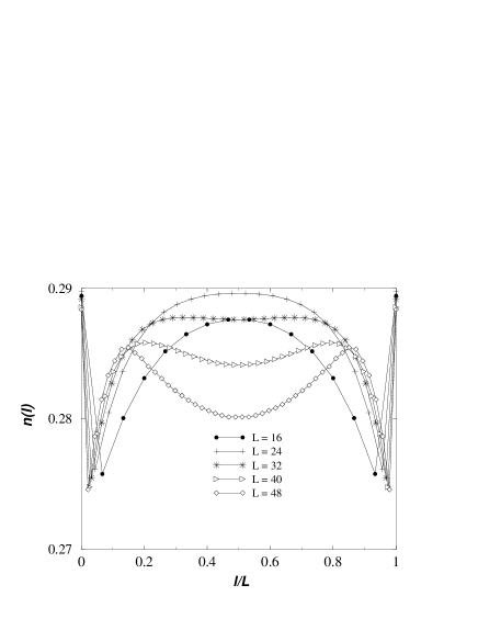
Figure 3: Particle density $n(l)$ at the estimated critical point $p_{c}=0.84036$ for an injection rate $p^{\prime}=0.03$ plotted as function of $l/L$.

Fig. 3 shows the particle density $n(l)$ as function of the scaled variable $l/L$ for an injection rate $p^{\prime}=0.03$, $L=16$, $24$, $32$, $40$ and $48$ at the estimated critical point $p=p_{c}$. The behaviour is now completely different with respect to the profiles with $p^{\prime}=0.3$. Apart from the two boundary sites (corresponding to $l=0$ and $l=L$), where the density of particles is weakly dependent on the system size $L$, we see that starting from the edges the density increases towards the bulk. For small systems the maximum of the density is found in the middle of the chain, while for systems large enough two maxima are located at a distance $l_{\rm max}\approx 7$ lattice spacings from the edges (we find that $l_{\rm max}$ is independent of $L$ for sufficiently long chains).

This phenomenon is rather counterintuitive since one would expect that the density of particles as a function of $l$ should decay monotonically starting from the edges and moving towards the center, as seen in figure 2 for $p^{\prime}=0.3$. The effect observed here actually has a counterpart in the magnetization profiles of equilibrium spin systems in the presence of a weak surface magnetic field weakh1 . This effect in turn was found and explained by appealing to the universal short-time critical dynamics involving the so-called slip exponent janssen . Non-monotonous profiles of this kind are a true fluctuation effect and cannot be explained on the level of a mean-field approximation, see weakh1 ; janssen ; diehl ; fredrik and appendix C. It is known, for instance for the Ising model at its critical point, that a weak surface field $h_{1}$ induces a macroscopic scale length $l_{1}$ such that up to a distance $l\approx l_{1}$ from the surface, the magnetization is increasing with $l$. It starts to decrease again as $l>l_{1}$, with the asymptotic behaviour $\sim l^{-\beta/\nu}$ for large distances (in the Ising model, $\nu_{\perp}=\nu_{\|}=\nu$) andrzej .

To describe non-monotonic densities of particles, it is necessary to modify the scaling form (39) to include a term depending on the boundary reaction rate $p^{\prime}$, following the standard theory of boundary critical phenomena at the ordinary transition, see weakh1 ; diehl . The rate $p^{\prime}$ will enter into the particle density in the form of a scaling variable $\lambda={p^{\prime}}l^{x_{1}}$, where $x_{1}$ is some scaling dimension. One expects the scaling form

$$n(l,p^{\prime})=l^{-\beta/\nu_{\perp}}{\cal F}(l/L,{p^{\prime}}l^{x_{1}})$$ (41)

Following the same analysis as presented in weakh1 ; diehl , one finds that $x_{1}=\beta_{1}/\nu_{\perp}$, with $\beta_{1}$ the (ordinary) order parameter surface exponent. This exponent has been calculated for directed percolation, see table 1, yielding $x_{1}\simeq 0.669$.

For large $\lambda$, one should recover from (41) the scaling form given in eq. (39), thus

$$\lim_{\lambda\to\infty}{\cal F}(l/L,\lambda)=F(l/L)$$ (42)

More interesting, for the present case, is the other limit where $\lambda\to 0$. In absence of particle injection ($p^{\prime}=0$), the particle density $n$ vanishes, which implies ${\cal F}(x,\lambda=0)=0$. At small $p^{\prime}$, it is natural to assume that the density varies linearly with $p^{\prime}$, leading to the condition

$${\cal F}(l/L,\lambda)\sim\lambda$$ (43)

valid in the range, say, $0\leq\lambda<\lambda_{0}$. Notice that $\lambda_{0}$ defines a length scale $l_{1}=(\lambda_{0}/p^{\prime})^{1/x_{1}}$. Therefore, in the $L\ll l_{1}$ limit, one finds

$$n(l,L)=l^{\rho^{\prime}}\widetilde{{\cal F}}(l/L)$$ (44)

obtained by inserting the limiting value (43) in eq. (41) and where $\rho^{\prime}=x_{1}-\beta/\nu_{\perp}=(\beta_{1}-\beta)/\nu_{\perp}$, in complete analogy with weakh1 .

From the numerical values quoted in table 1, we find $\rho^{\prime}\simeq 0.416$, the positivity of which explains the increase of the profiles with $l$ close to the boundary. Actually, the particle density with $p^{\prime}=0.03$ shown in Fig. 3 corresponds neither to the scaling regime (39) nor to (44), but to an intermediate situation.

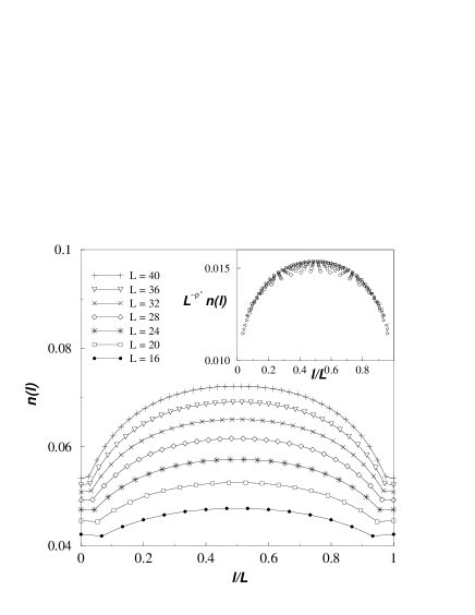
Figure 4: Density of particles at $p_{c}$ and for $p^{\prime}=0.002$. The inset shows the collapse of the scaled densities onto a single curve as expected from eq. (44).

In figure 4, we display the critical particle density for $L=16$, $20$, …$40$ but with a decreased injection rate $p^{\prime}=0.002$. Profiles are monotonously increasing from the edges and there is no sign of an inflection of the curves as seen in Fig. 3. The inflection point should be found at a distance from the edges $l_{\rm max}(p^{\prime}=0.002)$ given by the relation:

$$l_{\rm max}(p^{\prime}=0.002)=l_{\rm max}(p^{\prime}=0.03)\left(\frac{0.03}{0.002}\right)^{1/x_{1}}\approx 400$$

in units of the lattice constant, and where we have used $l_{\rm max}(p^{\prime}=0.03)\approx 7$ as estimated from the profiles of Fig. 3. Thus, we expect that for $p^{\prime}=0.002$, at about $400$ lattice spacings from the surface the density profiles should show a maximum and then start decreasing again. This effect should be noticeable only for systems of sizes $L>2l_{\rm max}\approx 800$, well beyond the range of sizes shown in figure 4.

The inset of figure 4 shows the scaled profiles $L^{-\rho^{\prime}}n(l)$ plotted as a function of the scaled distance $l/L$ (we have used the expected value of $\rho^{\prime}=0.416$ for directed percolation and removed the edge sites $l=0$ and $l=L$ from the plot). If the scaling assumptions leading to eq. (44) were correct, all the profiles for different values of $L$ should collapse into a single curve. Indeed, we find a trend towards a data collapse, although finite-size corrections are rather strong, especially in the middle of the chain, while they are weaker at the edges. It is remarkable, that the scaling law (44), whose derivation involves the scaling close to the boundary, should be valid for the entire finite system, at least for the lattice sizes under consideration here. On the basis of these observations, one may conclude that the dmrg data for the profiles agree with the results of the scaling theory also in the weak injection rate regime.

7.3 Profiles from matrix elements

So far, the calculations of the density profiles used the straightforward form (38) and then tried to perform the limit $p^{\prime}\to 0$ numerically, which in principle should be taken only after the $L\to\infty$ limit has been carried out. Alternatively, we may rely on an analogy with the calculation of the order parameter of equilibrium spin systems which avoids this cumbersome double limit Hame82 , see also Henk99 . If $|\psi_{1}^{(r)}\rangle$ and $\langle\psi_{1}^{(l)}|$ are the first excited eigenstates of $H$, consider NormN

$$N(l):=\langle\psi_{1}^{(l)}|{\hat{n}}(l)|\psi_{1}^{(r)}\rangle$$ (45)

where ${\hat{n}}(l)$ is the density operator at position $l$ and where we have simply set $p^{\prime}=0$. Although $N(l)$ is not directly related to the more “physical” density $n(l)$, it offers the distinct advantage that it is non-vanishing even for $p^{\prime}=0$ and furthermore displays the same scaling behaviour as expected for $n(l)$. Since in the percolating phase, the first gap $\Gamma$ is exponentially small for $L$ large, one might expect to find for $N(l)$ the same scaling behaviour as for $n(l)$. Indeed, as we shall see, the following finite-size scaling behaviour holds for $N(l)$ at $p=p_{c}$: $N(l)\sim L^{-\beta/\nu_{\perp}}$ for sites deep in the bulk, i.e. $l/L\simeq 1/2$ and $N(l)\sim L^{-\beta_{1}/\nu_{\perp}}$ for boundary sites, i.e. $l=0$ or $l=L$; with the same exponent values as found before.

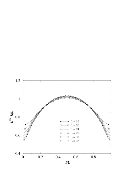
Figure 5: Plot of the scaled quantities $L^{\beta/\nu_{\perp}}N(l)$ as function of the scaled distance $l/L$ for $L=16,\ldots$ at the critical point $p=p_{c}$.

Figure 5 shows a scaling plot of $L^{\beta/\nu_{\perp}}N(l)$ as a function of $l/L$, where we used the value of $\beta/\nu_{\perp}=0.25208$ from table 1. The data collapse in a satisfactory way in the bulk, but rather poorly at the surface. This is consistent with our expectation of two different scaling regimes. It is also quite remarkable that the numerical data for $l=L/4$ and $l=3L/4$ show an almost perfect collapse.

We analyzed the numerical data at $p=p_{c}$ forming the finite-size estimates from two successive system sizes as done in eq. (36), using the values of $N(l)$ at $l=L/2$ and at the surface $l=1$. The data are listed in table 6. Extrapolation for $L\to\infty$ with the bst method yields $\beta/\nu_{\perp}=0.249(3)$ and $\beta_{1}/\nu_{\perp}=0.667(2)$, both in good agreement with the results quoted in table 1. Apparently the exponents extrapolated from $N(l)$ are more accurate than those obtained from the density profiles and allow a direct determination of surface exponents, allowing a comparison with field-theory methods per . Again, the data for $N(l)$ might also be used to find yet another estimate of $p_{c}$, but we have not carried out this calculation.

8 Conclusions

In this paper we have investigated the properties of two reaction- diffusion models at their critical point, by means of dmrg techniques. Our study demonstrates that the dmrg is capable to treat rather well out-of-equilibrium systems and provides a method for calculations of critical exponents, alternative to other general methods such as Monte Carlo simulations or series expansion techniques. The dmrg offers the advantages that (i) there is no critical slowing-down, (ii) the method does not require random numbers and (iii) there is no need to make any assumptions about the basic state around which one may expand.

Our findings may be summarised as follows.

(1) In the examples considered, the symmetric density matrix $\rho^{[1]}$ produced the most accurate results. It is essential to have a reliable method to diagonalize a sparse non-symmetric matrix. The non-symmetric Lanczos and the Arnoldi algorithms used here were found to produce results of comparable accuracy.

(2) It was enough to keep $m=32$ states. Improvements in numerical accuracy of the dmrg cannot be achieved by increasing $m$, but rather by enhancing the number of digits kept beyond the conventional 64-bit arithmetics.

(3) In order to analyse the critical region, it is essential to use the finite system method of the dmrg. The infinite system method alone is not sufficient.

(4) Finite-size data for critical non-equilibrium systems are strongly affected by finite-size corrections. Because usually the dmrg works best for free boundary conditions, finite-size corrections should be expected to be substantially larger than in calculations done with standard diagonalization techniques, which usually work with periodic boundary conditions. However, the trade-off is that from a single dmrg calculation one may get both bulk and surface exponents.

(5) In studies of the scaling of profiles, the consideration of matrix elements of the type of (45) may provide a better computational tool than the physically more straightforward profiles (38).

(6) Precise estimates of the location of the critical point and of critical parameters can only be obtained through a finite-sequence extrapolation technique. That requires a long sequence of precise lattice data for several distinct sizes, rather than data from a single large lattice.

(7) The extrapolation can be carried out reliably by the bst algorithm. The results for the critical exponents are in agreement with the results for series expansion and Monte Carlo simulation, see table 1. At present, the dmrg do not yet achieve the same precision as these. The precision of the method can be improved by generating longer chains. To overcome the numerical instabilities encountered, this will require to go beyond the usual 64-bit arithmetics.

All in all, we conclude that the dmrg has turned out to be a reliable general-purpose method, also for studying non-equilibrium critical phenomena, although it works best out of criticality.

Acknowledgements

We thank P. Fröjdh for fruitful correspondence and the Centre Charles Hermite of Nancy for providing substantial computational time. M.H. thanks A. Honecker for a very useful discussion.

Appendix A Relation with site and bond percolation

We recall the relationship of the reaction-diffusion processes defined in (1-5) with directed percolation. The latter is usually defined in terms of local probabilities giving the state of a site at time $t+1$ in terms of its two parent sites at time $t$

$$\mbox{${\begin{array}[]{c}\circ\;\circ\\ \bullet\end{array}}$}=0\;\;;\;\;\mbox{${\begin{array}[]{c}\bullet\;\circ\\ \bullet\end{array}}$}=p_{s}p_{b}\;\;;\;\;\mbox{${\begin{array}[]{c}\bullet\;\bullet\\ \bullet\end{array}}$}=p_{s}p_{b}(2-p_{b})$$ (46)

where $p_{s}$ and $p_{b}$ describe site and bond percolation, respectively. Here $\bullet$ marks an occupied and $\circ$ an empty site. Furthermore, $\mbox{${\begin{array}[]{c}\bullet\;\circ\\ \circ\end{array}}$}=1-\mbox{${\begin{array}[]{c}\bullet\;\circ\\ \bullet\end{array}}$}$ and so on. From these rules, a time evolution operator $S$, acting according to $|P(t+1)\rangle=S|P(t)\rangle$, is constructed, which is related to the quantum Hamiltonian $H=1-S$.

In order to link the percolation parameters $p_{s},p_{b}$ with the reaction and diffusion rates $\alpha,\beta,\gamma,\delta$ and $D$, we observe that the evolution of a site is according to (46) only dependent on its parentsand independent of the state of its neighbours at the same time $t$. Thus

$$\mbox{${\begin{array}[]{c}\bullet\;\circ\\ \bullet\end{array}}$}=\mbox{${\begin{array}[]{c}\bullet\;\circ\\ \bullet\;\circ\end{array}}$}+\mbox{${\begin{array}[]{c}\bullet\;\circ\\ \bullet\;\bullet\end{array}}$}=\mbox{${\begin{array}[]{c}\bullet\;\circ\\ \circ\;\bullet\end{array}}$}+\mbox{${\begin{array}[]{c}\bullet\;\circ\\ \bullet\;\bullet\end{array}}$}$$ (47)

by summing over the possible states of the right or left nearest neighbours. Similar relations hold for the other rates. From this, the following conditions for a mapping of the process (1-5) onto directed percolation hold

$$\beta=1-\delta=p_{s}p_{b}\;\;;\;\;D=0\;\;;\;\;2\alpha+\gamma=1-p_{s}p_{b}(2-p_{b})$$ (48)

It is easy to check that the model (13) cannot be exactly mapped onto directed percolation this way, although it still is in the same universality class. For example, a mapping onto site percolation ($p_{b}=1$) requires that $\delta=2\alpha+\gamma$, while bond percolation ($p_{s}=1$) is achieved for $\delta^{2}=2\alpha+\gamma$.

Appendix B On the density matrix

To justify the use of the density matrix $\widehat{\mbox{\rm tr\,}}|\psi_{0}\rangle\langle\psi_{0}|$, one writes the targeted state in a product state of states $|\alpha_{l},i_{l}\rangle\equiv|i\rangle$ of the “system” one wants to describe and $|j_{r},\beta_{r}\rangle\equiv|j\rangle$ of the “environment”. From the construction of the dmrg, each of the bases has $mn$ elements, where $n$ is the number of states per site. Then

$$|\psi_{0}\rangle=\sum_{ij}\psi_{0}(i,j)|i\rangle|j\rangle$$ (49)

One now approximates $|\psi_{0}\rangle$ by $|\tilde{\psi}_{0}\rangle$, with

$$|\tilde{\psi}_{0}\rangle=\sum_{\alpha,j}\tilde{\psi}_{0}(\alpha,j)|\alpha\rangle|j\rangle$$ (50)

where the sum over $\alpha$ runs over $m$ orthogonal states in the system basis, $|\alpha\rangle=\sum_{i}u_{\alpha i}|i\rangle$. One now demands that the approximation is optimal by minimising

$$\||\psi_{0}\rangle-|\tilde{\psi}_{0}\rangle\|^{2}=1-2\sum_{\alpha ij}\tilde{\psi}_{0}^{2}(\alpha,j).$$ (51)

Making this stationary with respect to $\tilde{\psi}_{0}(\alpha,j)$ gives $\sum_{i}\psi_{0}(i,j)u_{\alpha i}=\tilde{\psi}_{0}(\alpha,j)$ and thus the global minimum of

$$\||\psi_{0}\rangle-|\tilde{\psi}_{0}\rangle\|^{2}=1-\sum_{\alpha ii^{\prime}}u_{\alpha i}\rho(i,i^{\prime})u_{\alpha i^{\prime}}$$ (52)

has to be found. Here one introduces the reduced density matrix

$$\rho(i,i^{\prime})=\sum_{j}\psi_{0}(i,j)\psi_{0}(i^{\prime},j).$$ (53)

The stationary points of (52) are obviously given by setting $|\alpha\rangle$ equal to the eigenvectors of the reduced density matrix (Ritz condition). The stationary values of (52) are then given by $1-\sum_{i=1}^{m}\lambda_{i}$, where $\lambda_{i}$ are the eigenvalues of the density matrix ($0\leq\lambda_{i}\leq 1$, $\sum\lambda_{i}=1$). The global minimum is obtained by choosing the $m$ eigenvectors with the largest associated eigenvalues.

In the non-symmetric case, repeating the same argument, one finds that the minimization of:

$$\||\psi_{i}^{(l)}\rangle-|{\tilde{\psi}}_{i}^{(l)}\rangle\|^{2}+\||\psi_{i}^{(r)}\rangle-|{\tilde{\psi}}_{i}^{(r)}\rangle\|^{2}$$ (54)

yields as optimal basis set the eigenvectors of the density matrix (30).

Appendix C Density profiles from kinetic equations

We show that for branching-fusing (13), the mean field steady-state density profile for the semi-infinite system $x\geq 0$ with a prescribed boundary density is a monotonous function of the distance $x$ from the boundary. If $a(x,t)$ is the mean particle density, the kinetic equation is

$$\dot{a}=Da^{\prime\prime}+4(p-1/2)\,a-2a^{2}$$ (55)

In the steady state, $\dot{a}=0$. We write $a(x)=a_{\infty}\varphi(x/\xi_{\perp})$, where $a_{\infty}=2p-1\sim\xi_{\perp}^{-2}$ is the bulk density and $\xi_{\perp}=\sqrt{D/(p-1/2)}$ the spatial correlation length. The profile is

$$\varphi(y)=\frac{3}{2}\left(\frac{\sqrt{(2\varphi_{0}+1)/3\,}+\tanh(y)}{1+\sqrt{(2\varphi_{0}+1)/3\,}\,\tanh(y)}\right)^{2}-\frac{1}{2}$$ (56)

where $\varphi_{0}=a(0)/a_{\infty}$ is related to the boundary density. Evidently, $\varphi(y)\to 1$ as $y\to\infty$ monotonously. The above result was derived for a semi-infinite system with $p>p_{c,{\rm MF}}=1/2$. For a finite system at $p=1/2$, the $p$-dependence of the correlation length $\xi_{\perp}$ is traded for a size-dependence.

References

- (1) S. R. White, Phys. Rev. Lett. 69, 2863 (1992); Phys. Rev. B 48, 10345 (1993).
- (2) S.R. White, D.A. Huse, Phys. Rev. B48, 3844 (1993); S. R. White, R. M. Noack and D. J. Scalapino, Phys. Rev. Lett. 73, 886 (1994); E.S. Sørensen, I. Affleck, Phys. Rev. Lett. 71, 1633 (1993); U. Schollwöck, Th. Jolicœur, Europhys. Lett. 30, 493 (1995); S. Moukouri and L.G. Caron, Phys. Rev. Lett. 77, 4640 (1996); K. Hallberg, X.Q.G. Wang, P. Horsch and A. Moreo, Phys. Rev. Lett. 76, 4955 (1996).
- (3) T. Nishino, J. Phys. Soc. Jpn. 64, L3598 (1995); E. Carlon and A. Drzewiński, Phys. Rev. Lett. 79, 1591 (1997).
- (4) I. Peschel, K. Hallberg, X. Wang (eds.): Proceedings of the First International dmrg Workshop (Springer Lecture Notes of Physics, 1999).
- (5) R.J. Bursill, T. Xiang and G.A. Gehring, J. Phys. Cond. Mat. 8, L583 (1996); X. Wang and T. Xiang, Phys. Rev. B56, 5061 (1997); N. Shibata, J. Phys. Soc. Jpn. 66, 2221 (1997); K. Maisinger and U. Schollwöck, Phys. Rev. Lett. 81, 445 (1998).
- (6) Y. Hieida, J. Phys. Soc. Jpn. 67, 369 (1998).
- (7) M. Kaulke and I. Peschel, Eur. Phys. J. B5, 727 (1998)
- (8) V. Privman (Ed) Finite-Size Scaling and Numerical Simulation of Statistical Systems, World Scientific (Singapore 1990)
- (9) J.L. Cardy (Ed) Finite-Size Scaling North Holland (Amsterdam 1988)
- (10) M. Henkel, Conformal Invariance and Critical Phenomena, Springer (Heidelberg 1999)
- (11) M. Henkel, E. Orlandini and J. Santos, Ann. of Phys. 259, 163 (1997)
- (12) N.G. van Kampen, Stochastic Processes in Physics and Chemistry, (2nd ed.) North Holland (Amsterdam 1997)
- (13) M. Cieplak, M. Henkel, J. Karbowski and J.R. Banavar, Phys. Rev. Lett. 80, 3654 (1998)
- (14) F.C. Alcaraz, M. Droz, M. Henkel and V. Rittenberg, Ann. of Phys. 230, 250 (1994)
- (15) Unless explicitly stated otherwise, right vectors and left vectors are not considered to be related by hermitian conjugation.
- (16) J.W. Essam, A.J. Guttmann, I. Jensen and D. Tanlakishani, J. Phys. A29, 1619 (1996).
- (17) M.A. Muñoz, R. Dickman, A. Vespignani and S. Zapperi, preprint cond-mat/9811287
- (18) K.B. Lauritsen, K. Sneppen, M. Markosová and M.H. Jensen, Physica A 246, 1 (1997).
- (19) S. Östlund and S. Rommer, Phys. Rev. Lett. 75, 3537 (1995).
- (20) E. Carlon and F. Iglói, Phys. Rev. B57, 7877 (1998).
- (21) G.H. Golub, C.F. van Loan, Matrix Computations (3rd ed.), Baltimore, 1996
- (22) The package can be found in ftp://caam.rice.edu in the directory pub/people/software/ARPACK.
- (23) E. Domany and B. Schaub, Phys. Rev. B29, 4095 (1984)
- (24) M. Henkel and H.J. Herrmann, J. Phys. A23, 3719 (1990)
- (25) R. Burlisch and J. Stoer, Numer. Math. 6, 413 (1964).
- (26) M. Henkel and G. Schütz, J. Phys. A21, 2617 (1988).
- (27) M.N. Barber and C.J. Hamer, J. Austr. Math. Soc. B23, 229 (1982).
- (28) M. Fisher and P. G. de Gennes, C. R. Acad. Sci. Paris B 287, 207 (1978).
- (29) U. Ritschel and P. Czerner, Phys. Rev. Lett. 77, 3645 (1996)
- (30) H. K. Janssen, B. Schaub and B. Schmittmann, Z. Phys. B73, 559 (1989).
- (31) U. Ritschel and H. W. Diehl, Nucl. Phys. B 464, 512 (1996).
- (32) F. van Wijland, K. Oerding and H. J. Hilhorst, Physica A 251, 179 (1998).
- (33) These phenomena were recently studied by dmrg in two-dimensional Ising strips: A. Maciołek, A. Ciach and A. Drzewiński, preprint.
- (34) C.J. Hamer, J. Phys. A15, L675 (1982)
- (35) Here, the eigenvectors were normalized according to .
- (36) K. Lauritsen, P. Fröjdh and M. Howard, Phys. Rev. Lett. 81, 2104 (1998); P. Fröjdh, M. Howard and K. Lauritsen, J. Phys. A31, 2311 (1998).