Slave fermion theory of confinement in strongly anisotropic systems

Abstract

We present a mean field treatment of a strongly correlated model of electrons in a three–dimensional anisotropic system. The mass of the bare electrons is larger in one spatial direction (the $c$–axis direction), than in the other two (the $ab$–planes). We use a slave fermion decomposition of the electronic degrees of freedom and show that there is a transition from a deconfined to a confined phase in which there is no coherent band formation along the $c$–axis.

The Date

One of the most controversial, and hard to understand, problems related with high-$T_{c}$ cuprates is the anomalous charge transport observed experimentally[1]. The charge dynamics reflects the anisotropy in the crystal structure of these compounds, which consists of weakly coupled planes. In the usual notation, we will refer to “$c$–axis” and “$ab$–planes” as the directions transverse and parallel to the planes respectively. The in–plane conductivity $\sigma_{ab}$ shows a behavior characteristic of the metallic state. On the other hand, close to the insulating state, in the so called underdoped regime, the $c$–axis conductivity $\sigma_{c}$ is “incoherent”: the values of $\sigma_{c}$ are below the minimum metallic conductivity[2], the temperature dependence is anomalous, and the frequency dependence does not show signatures of Drude–like behavior[3, 4].

Band structure calculations indicate an anisotropy which, within the framework of Boltzman transport, imply metallic behavior with an anisotropy $\sigma_{c}/\sigma_{ab}$ well above the experimental observation. Perturbative treatments within the Fermi–liquid theory indicate that the anisotropy is not renormalized by interactions[5]. Perhaps the main objection to the “conventional” theories of $c$–axis transport[7, 8] is the observed value of the anisotropy of the conductivity. In the superconducting phase coherence is reestablished in all directions[9]. This lead Anderson and others to attribute the anomalies in transport in the normal state to the effect of strong electronic correlations, and to conclude that in order to describe the incoherent $c$–axis conductivity the Fermi–liquid picture should be abandoned. The starting point used as a paradigm is the one-dimensional correlated problem where it is rigorously known that the Fermi–liquid picture fails. Considerable work has been done in weakly coupled chains that suggest that a state can be formed in which the coherence is confined to the motion along the chains, the motion transverse to the chains being incoherent[6].

A complete theory for the charge dynamics in anisotropic strongly correlated systems is not yet available. Due to the complexity of the problem, much work remains to be done in order to develop a fully consistent and controlled calculation scheme that could account for the phenomenology indicated by the experiments. In the mean time, the analisys of simple models is useful as a starting point towards the final answer. Here we present a mean field treatment of a system of coupled planes that includes the strong anisotropy, and incorporates the strong correlations responsible for the non–Fermi liquid behavior. We show that, within that mean field, a transition from a deconfined to a confined phase takes place. The parameter signaling the transition is the gain in kinetic energy due to band formation in the $c$–axis direction.

We consider the Hubbard model in the limit of infinite on–site repulsion, described by the following Hamiltonian

$$H=\sum_{\langle i,j\rangle}t_{i,j}\sum_{\sigma}(1-n_{i,-\sigma})c_{i,\sigma}^{\dagger}c_{j,\sigma}(1-n_{j,-\sigma}),$$ (1)

where $\langle i,j\rangle$ refers to near neigbors on a cubic lattice where the anisotropy is incorporated in the values of hopping the matrix elements: $t_{i,j}=t_{\|}$ for in–plane hoppings and $t_{i,j}=t_{\bot}$ for the motion along the $c$–axis. The fermion operators $c_{i,\sigma}^{\dagger}$ create an electron at site $i$ only if the site is empty.

A well known mean field description of Hamiltonian 1 is the slave–boson[10, 11] approach in which each local configuration has associated with it a fermionic or bosonic degree of freedom, such that $c_{i,\sigma}^{\dagger}=a_{i,\sigma}^{\dagger}e_{i}$, where $a_{i,\sigma}^{\dagger}$ creates a fermion with spin $\sigma$ at the $i$–th site representing a singly occupied configuration, and $e_{i\text{ }}$destroys a boson  representing the empty state at the same site. A standard mean field calculation decouples fermions and bosons and relaxes the exact constraint of one “particle” (fermion + boson) per site. The resulting problem is that of non–interacting bosons and fermions self–consistently coupled. As a result the ideal bosons condensate in a $k=0$ state, the overall effect being a renormalization of the masses of the fermions. It is important to note that, even for an anisotropic system, the $k=0$ bosonic ground state wave function does not know about the anisotropy, and the mass renormalization is the same in all spatial directions. Consequently, such an approach preserves the anisotropy and the Fermi liquid character of the ground state. At least formally, one can conceive corrections to this state that improve the treatment of the constraint to avoid multi–occupancy of the particles at the same site. There are, however, other alternative treatments that–still within the mean field level–take into account the hard core constraint for the bosons exactly. In the present work we present a mean field along this line. In what follows we show that at an alternative description in terms of slave–fermions  for the infinite–$U$ case breaks the Fermi liquid description and produces a confined coherent sate[12] in the $ab$ planes.

We introduce a description in which the original projected fermions are represented by three fermions:

$$\overline{c}_{i,\sigma}\equiv c_{i,\sigma}(1-n_{i,-\sigma})=a_{i,\sigma}f_{i,\uparrow}^{\dagger}f_{i,\downarrow}$$ (2)

The above representation respects the anticommutation relation between the projected operators $\overline{c}_{i,\sigma}$ and $\overline{c}_{i,\sigma}^{\dagger}$ provided one stays within the physical Hilbert space. A related fermion linearization was presented in Ref. [13].

The product $f_{i,\uparrow}^{\dagger}f_{i,\downarrow}$ is a spin flip operator corresponding to a pseudo–spin degree of freedom not related to $\sigma$. When this fictitious spin is $\downarrow$ in site $i$ this means that the site is occupied, and the site is empty if the spin is $\uparrow$: there are as many $f_{\downarrow}$’s as there are electrons and as many $f_{\uparrow}$’s as there are holes. The $f$ fermions therefore satisfy

$$\langle f_{i,\uparrow}^{\dagger}f_{i,\uparrow}\rangle+\langle f_{i,\downarrow}^{\dagger}f_{i,\downarrow}\rangle=1,\text{ }\sum_{\sigma}\langle a_{i,\sigma}^{\dagger}a_{i,\sigma}\rangle+\langle f_{i,\downarrow}^{\dagger}f_{i,\downarrow}\rangle=1,$$ (3)

and, in turn

$$\sum_{\sigma}\langle a_{i,\sigma}^{\dagger}a_{i,\sigma}\rangle=1-\delta,$$ (4)

with $\delta$ representing the fractional deviation in occupation number with respect to the half–filling case of one electron per site.

At the mean field level the ground state wave function consists of a direct product of three Fermi seas, one per each of the fermion degrees of freedom. The total energy in this approximation is given by

$$E_{0}=-\sum_{\langle i,j\rangle}t_{i,j}A_{i,j}\chi_{i,j}^{2},$$ (5)

with

$$A_{i,j}=\sum_{\sigma}\langle a^{\dagger}_{i,\sigma}a_{j,\sigma}\rangle,$$ (6)

$$\chi_{i,j}=\langle f^{\dagger}_{i,\uparrow}f_{j,\uparrow}\rangle=\langle f^{\dagger}_{i,\downarrow}f_{j,\downarrow}\rangle,$$ (7)

where the last equality holds because we are dealing with a bipartite lattice with particle–hole symmetry. The three species of fermions are free with their hopping amplitudes renormalized by the factors $A_{i,j}$, and $\chi_{i,j}$. These factors are responsible for renormalizing the anisotropy and can be better visualized in the mean field Hamiltonian

$$H_{{\rm MF}}=-\sum_{\langle i,j\rangle}t_{i,j}\sum_{\sigma}\left[\chi_{i,j}^{2}a^{\dagger}_{i,\sigma}a_{j,\sigma}+A_{i,j}\chi_{i,j}f^{\dagger}_{i,\sigma}f_{j,\sigma}\right]+C,$$ (8)

with $C$ a constant.

Note that, for small deviations from half filling, the $f_{i,\uparrow}$ ($f_{i,\downarrow}$) fermions are moving close to the bottom (top) of their band, whereas the $a$ fermions are close to the center of the band. This makes their respective Fermi surfaces different.

Our mean field can be understood in two steps. First the $a$ fermions are decoupled from the $f$ fermions. At that level, the $a$ fermions are free, but the $f_{\uparrow}$ fermions and the $f_{\downarrow}$ fermions are strongly correlated. The dynamics of the system of $f$ fermions at this level is identical to that of an $xy$–model, and can be mapped onto a hard–core boson problem. In the second step the $f$ fermions of different spin are decoupled and treated as free fermions (with a self consistent constraint on the dynamics)[14]. Note that, at the level of step one, the above mentioned system of hard–core bosons will in principle have an anisotropy in the expectation values of the kinetic energy terms that will depend on direction. This is due to the quantum fluctuations introduced by the hard–core constraint.

At half filling ($\delta=0$), the kinetic energy of the $f$ fermions is zero, the renormalization factor $\chi_{ij}=0$, giving the localized limit of the $a$ fermions which we identify as the Mott insulating state. On the other hand, far from half filling, for $\delta\sim 1$, the density of $a$ –fermions is so low that they should behave as non–interacting, but our mean field fails to recover this limit. Decoupling the $f$–fermions from the $a$–fermions is not a good approximation in the limit of high doping $\ \delta$ because the probability of finding an $f_{\downarrow}$-fermion at a site occupied by an $a$ fermion is very low [$\sim(1-\delta)^{2}$], while the exact dynamics requires this probability to be one. Therefore our results will be valid close to half filling, or $\delta\sim 0$.

Due to translational invariance, the ground state energy will be a function of the four quantities $A_{\|}$, $A_{\bot}$, $\chi_{\|}$ and $\chi_{\bot}$:

$$E_{0}=-4t_{\|}A_{\|}\chi_{\|}^{2}-2t_{\bot}A_{\bot}\chi_{\bot}^{2}.$$ (9)

The one particle energies of the $f$ and $a$ fermions are respectively

$$E_{{\bf k}}^{f}=t_{\|}A_{\|}\chi_{\|}\varepsilon_{k_{\|}}-t_{\bot}A_{\bot}\chi_{\bot}2\cos k_{z},$$ (10)

$$E_{{\bf k}}^{a}=t_{\|}\chi_{\|}^{2}\varepsilon_{k_{\|}}-t_{\bot}\chi_{\bot}^{2}2\cos k_{z},$$ (11)

with

$$\varepsilon_{k_{\|}}=-2(\cos k_{k}+\cos k_{y}).$$ (12)

Effective chemical potentials $\lambda$ and $\mu$ have to be determined for each of the two types of fermions through the equations

$${\frac{1}{N}}\sum_{{\bf k}}f(E_{{\bf k}}^{f}-\lambda)=\delta,\;\;\;\;\;\;\;\;{\frac{1}{N}}\sum_{{\bf k}}f(E_{{\bf k}}^{a}-\mu)={\frac{1-\delta}{2}}.$$ (13)

We approximate the reduced density of states corresponding to the motion within the plane by a constant: $\sum_{k_{\|}}\delta(\varepsilon-\varepsilon_{k_{\|}})=\Theta(4-|\varepsilon|)/4$, and find that the mean field equations can be written in terms of the parameters $\alpha$ and $\beta$ defined as

$$\alpha={\frac{t_{\bot}}{t_{\|}}}{\frac{A_{\bot}\chi_{\bot}}{A_{\|}\chi_{\|}}},\;\;\;\;\;\;\;\;\;\beta={\frac{t_{\bot}}{t_{\|}}}\left({\frac{\chi_{\bot}}{\chi_{\|}}}\right)^{2}.$$ (14)

After straightforward integrations, and using the fact that close to half filling the Fermi surface of the $a$ fermions is open, the mean field equations are

$$A_{\|}={\frac{1}{2}}(1-\delta^{2})-\left({\frac{\beta}{2}}\right)^{2}\;,\;\;\;\;\;A_{\bot}={\frac{\beta}{4}},$$ (15)

$$\chi_{\|}={\frac{1}{8\pi}}\left\{\left[1-\left({\frac{\widetilde{\lambda}}{4}}\right)^{2}\right]2k_{0}-{\frac{\alpha^{2}}{4}}\left(k_{0}+{\frac{1}{2}}\sin 2k_{0}\right)-{\frac{\widetilde{\lambda}\alpha}{2}}\sin k_{0}\right\},$$ (16)

$$\chi_{\bot}={\frac{1}{4\pi}}\left\{\left(1-{\frac{\widetilde{\lambda}}{4}}\right)2k_{0}\sin k_{0}+{\frac{\alpha}{2}}\left(k_{0}+{\frac{1}{2}}\sin 2k_{0}\right)\right\},$$ (17)

with $\widetilde{\lambda}=\lambda/(t_{\|}A_{\|}\chi_{\|})$ determined from the equation

$$\delta={\frac{1}{8\pi}}\left\{(\widetilde{\lambda}+4)k_{0}+2\alpha\sin k_{0}\right\},$$ (18)

and $k_{0}=\cos^{-1}[-(\widetilde{\lambda}+4)/2\alpha]$ for $|(\widetilde{\lambda}+4)/2\alpha|<1$ and $\pi$ otherwise. Note that $\alpha$ plays the role of an effective anisotropy of the $f$–fermions. For a given $\delta$, if we fix $\alpha$, the renormalization factors $\chi$ and $A$ are determined by the Equations (15) through (18). This means that $\alpha$ plays the role of a variational parameter with respect to which we have to minimize the energy $E_{0}$. As an example, in Figure 2 we show some curves of $E_{0}$ vs. $\alpha$ for different values of doping using as a parameter the bare anisotropy $t_{\bot}/t_{\|}$.

The curves indicate that for fixed $t_{\bot}/t_{\|}$ there is a discontinuous jump in the position of the minimum of $E_{0}$ as $\delta$ is varied. The curve shown in Figure 2 for $\delta=0.002$ corresponds to the confined phase for which $\alpha=0$, and the renormalization factor $\chi_{\bot}=0$. The curve for $\delta=0.0018$ has its minumum at finite $\alpha$ and hence corresponds to a three dimensional metal with a renormalized anisotropy.

A phase diagram that result from our calculation is shown in Figure 3

A very important point is to establish that the particle motion does not correspond to a Fermi liquid. We show this by computing the form of the occupation number of the original fermions in the confined phase within our mean–field squeme:

$\displaystyle n_{k,\sigma}\equiv\langle c_{k,\sigma}^{\dagger}c_{k,\sigma}\rangle=\frac{n}{2}+\frac{1}{N}\sum_{i\neq j}e^{ik(R_{i}-R_{j})}\langle c_{i,\sigma}^{\dagger}c_{j,\sigma}\rangle$with $n$ the particle density. The term $\langle c_{i,\sigma}^{\dagger}c_{j,\sigma}\rangle$ is evaluated using the representation of Equation 2. In mean field the result is a convolution of the occupation numbers of the three fermions ($f$’s and $a$). Using the constraints of Equations 3 and 4 one obtains

$\displaystyle n_{k,\sigma}=\frac{1-\delta}{2}\left[1-\delta(1-\delta)\right]+\frac{1}{N^{2}}\sum_{pq}n_{p,\sigma}^{(a)}n_{q,\downarrow}^{(f)}n_{p+q-k,\uparrow}^{(f)}.$

The occupation numbers above correspond to three Fermi surfaces. For small $\delta$ the Fermi surfaces corresponding to the $f$ fermions are are two circles centered respectively at ${\bf k=(}0,0)$ and ${\bf k=(}\pi,\pi)$. On the other hand, the Fermi surface of the $a$ fermions are close to a diamond. The result of the convolution above (See Figure 4) is that $n_{k,\sigma}$ does not have a discontinuity, implying an non–Fermi liquid state.

A few points related to the calculation deserve a comment:

i) Due to the approximation made in the density of states we cannot recover the isotropic case. The approximation used is aimed at describing anisotropic systems.

ii) In our calculation the confined regime is identified by the vanishing of the expectation value of the interplane hopping indicating that there is not band formation along this direction. We interpret this result as an indication of incoherence, even though one expects some interplane–coupling to remain in the exact incoherent regime. The picture is analog to the slave boson description of the Mott insulator. There, the insulating state is characterized by a vanishing of the inter–site hopping, while we know that in the exact ground state this magnitude is small but finite.

In summary, we have presented a mean field calculation and derived a phase–diagram of a strongly interacting anisotropic system. We have shown that, as the anisotropy increases, for small deviations from half filling a transition takes place from a deconfined phase to a confined phase in which the motion in the $c$–axis direction is completely incoherent while the motion in the $ab$–direction corresponds to a coherent, non–Fermi liquid state.

FIG. 1.: Schematic rendition of the slave fermion decomposition. When an $a$ fermion hops from site $i+1$ to site $i$, there is a spin–flip of $f$ fermions represented by the dashed arrows. The upper (lower) part of the figure represents the configuration before (after) the hopping process.

FIG. 2.: Ground state energy vs. the variational parameter $\alpha$for an anisotropy of $t_{\bot}/t_{\|}=0.3$ and the indicated values of doping.

FIG. 3.: Phase diagram valid in the low doping regime indicating the boundary between a confined phase and a three–dimensional anisotropic phase.

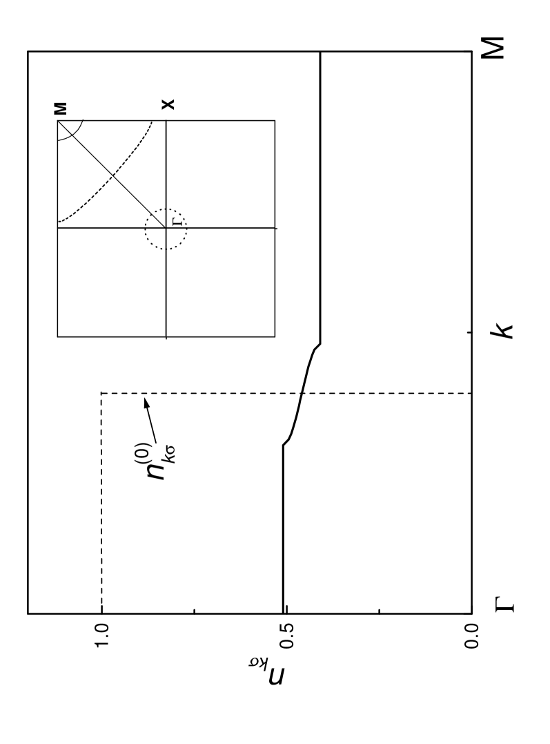
FIG. 4.: Fermion occupation number vs. wave vector in the direction marked in the inset. The dashed line shows the bare, non–interacting, occupation number. Note that there is no discontinuity in $n_{k,\sigma}$, as expected in a non–Fermi–liquid state. The inset also shows the Fermi surfaces–in the first quadrant only–of the $f$ fermions (small circle shown in short dashed and arc in continuous line close to the $M$ point) and of the $a$ fermions (dashed line).

REFERENCES

- [1] P. W. Anderson, THE Theory of Superconductivity in the High– Cuprates, Princeton University Press, 1997.
- [2] A. J. Leggett, Braz. J. Phys. 22, 129 (1992)
- [3] C. C. Homes, T. Timusk, R. Liang, A. Bonn and W. N. Hardy, Phys. Rev. Lett. 71 1645 (1993).
- [4] For a review of experiments see S. L. Cooper and K. E. Gray, in Physical Properties of High Superconductors, vol. , edited by D. M. Grinsberg (World Scientific, Singapore, 1994).
- [5] R. Shankar, Rev. Mod. Phys. 66, 129 (1994).
- [6] D. S. Clarke, S. P. Strong, and P. W. Anderson, Phys. Rev. Lett. 20 3218 (1994).
- [7] M. J. Graf, D. Rainer, and J. A. Sauls, Phys. Rev. B 47, 12089 (1993).
- [8] A. G. Rojo and K. Levin, Phys. Rev. B 48, 16861 (1993).
- [9] S. Chakravarty et al., Science 261, 337 (1993).
- [10] P. W. Anderson, Science 235, 1196 (1987).
- [11] J. J. Vicente Alvarez, C. A. Balseiro and H. A. Ceccatto, Phys. Rev. B 54, 11207 (1996); ibid. 56, 1141.
- [12] D. G. Clarke and S. P. Strong, Adv. in Phys. 46, 545 (1997).
- [13] P. Zanardi, J. Phys. A 29 541 (1996).
- [14] J. B. Marston and I. Affleck, Phys. Rev. B, 39,11538 (1989).