Extremal Optimization of Graph Partitioning at the Percolation Threshold

Abstract

The benefits of a recently proposed method to approximate hard optimization problems are demonstrated on the graph partitioning problem. The performance of this new method, called Extremal Optimization, is compared to Simulated Annealing in extensive numerical simulations. While generally a complex (NP-hard) problem, the optimization of the graph partitions is particularly difficult for sparse graphs with average connectivities near the percolation threshold. At this threshold, the relative error of Simulated Annealing for large graphs is found to diverge relative to Extremal Optimization at equalized runtime. On the other hand, Extremal Optimization, based on the extremal dynamics of self-organized critical systems, reproduces known results about optimal partitions at this critical point quite well.

]

I Introduction

The optimization of systems with many degrees of freedom with respect to some cost function is a frequently encountered task in physics and beyond [1]. In cases where the relation between individual components of the system is frustrated [2], such a cost function often exhibits a complex “landscape” [3] over the space of all configurations. For growing system size, the cost function may exhibit an exponentially increasing number of unrelated local extrema separated by sizable barriers which makes the search for the exact, optimal solution usually unreasonably costly. Thus, it is of great importance to develop fast and reliable methods to find near-optimal solutions for such problems.

The observation of certain physical processes, in particular the annealing of disordered materials, have lead to general-purpose optimization methods such as “simulated annealing” (SA) [5, 6]. SA applies the formalism of equilibrium statistical mechanics and in principle only requires the cost function as input. Thus, it is applicable to a variety of problems. But the performance of SA is hard to assess in general, even when limited to the standard combinatorial optimization problems. Aside from a multitude of adjustable parameters that crucially determine the quality of SA’s performance in a particular context, typical combinatorial optimization problems themselves possess various parameters that may change the landscape and SA’s behavior drastically [7].

In this paper we will explore the properties of a new general-purpose method, called Extremal Optimization (EO) [4], in comparison with SA. In contrast to SA, EO is based on ideas from non-equilibrium physics. As the basis for comparison we will use the graph partitioning problem (GPP), a standard NP-hard combinatorial optimization problem [8] with similarities to disordered spin systems. We find that the GPP has a critical point as a function of the connectivity of graphs, with a less complex phase at lower connectivities. This critical point is related to the percolation transition of the graphs. Near this critical point, the performance of SA markedly deteriorates while EO produces only small errors.

This paper is organized as follows: In the next section we describe the philosophy behind the EO method, in Sec. III we introduce the graph partitioning problem, and Sec. IV we present the algorithms and the results obtained in our numerical comparison of SA and EO, followed by conclusions in Sec. V.

II Extremal Optimization

EO provides an entirely new approach to optimization [4], based on the non-equilibrium dynamics of systems exhibiting self-organized criticality (SOC)[9]. SOC often emerges when a system is dominated by the evolution of extremely atypical degrees of freedom [10].

A simple example of such a dynamical system which inspired the development of EO is the Bak-Sneppen model [11]. There, species are represented by a number between 0 and 1 that indicates their “fitness,” located on the sites of a lattice. The smallest number (representing the worst adapted species) at each update is discarded and replaced with a new number drawn from a uniform distribution on $[0,1]$. Without any interactions, all the numbers in the system would eventually become 1. But obvious interdependencies between species provide constraints for balancing the systems’ fitness with that of each species: The change of fitness in one species impacts the fitness of an interrelated species. In the Bak-Sneppen model, the fitness values on all sites neighboring the smallest number at that time step are simply replaced with new random numbers as well [12]. After a certain number of such updates, the system organizes itself into a highly correlated state known as self-organized criticality (SOC) [9].

In the SOC state, almost all species have reached a fitness above a certain threshold. But these species merely possess what is referred to as punctuated equilibrium [11, 13], because the co-evolutionary activity is bound to return in a chain reaction where a weakened neighbor can undermine one’s own fitness. Fluctuations that rearrange the fitness of many species abound and can rise to the size of the system itself, making any possible configuration accessible. Hence, such non-equilibrium systems provide a high degree of adaptation for most entities in the system without limiting the scale of change towards even better states.

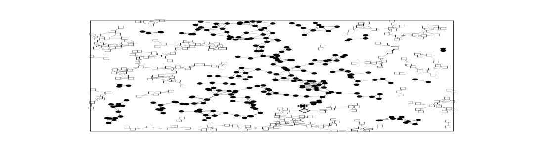
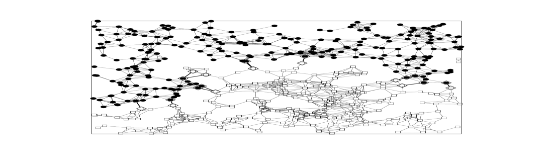
FIG. 1.: Two random geometric graphs, $N=500$, with $\alpha=4$ (top) and $\alpha=8$ (bottom) in an optimized configuration found by EO. At $\alpha=4$ the graph barely percolates, with merely one “bad” edge (between points of opposite sets, masked by diamonds) connecting a set of 250 round points with a set of 250 square points, thus $m_{\rm opt}=1$. For the denser graph on the bottom, EO reduced the cutsize to $m_{\rm opt}=13$.

EO attempts to utilize this phenomenology to obtain near-optimal solutions for optimization problems [14]. For instance, in a spin glass system [1] we may consider as fitness for each spin its contribution to the total energy of the system. EO would search for ground state configurations by perturbing preferentially spins with large contributions. Like in the Bak-Sneppen model, such perturbations would be local, random rearrangements of those poorly adapted spins, allowing for better as well as for worse outcomes at each update. In the same way as systems exhibiting SOC get driven recurrently towards a small subset of attractor states through a sequence of “avalanches” [15, 9], EO can fluctuate widely to escape local optima while the extremal selection process ensures recurrent approaches to many near-optimal configurations. Especially in exploring low temperature properties of disordered spin systems, those qualities may help to avoid the extremely slow relaxation behavior faced by heat bath based approaches [16]. In that, EO provides an approach alternative – and apparently equally capable [4] – to Genetic Algorithms, which are often the only means to illuminate those important properties [17]. The partitioning of sparse graphs as discussed here is particularly pertinent in preparation for similar studies on actual spin glasses.

It has been observed that many optimization problems exhibit critical points that separate off phases with simple cases of a generally hard problem [18]. Near such a critical point, finding solutions becomes particularly difficult for local search methods which proceed by exploring for an existing solution some neighborhood in configuration space. There, near-optimal solutions become widely separated with diverging barrier heights between them. It is not surprising that search methods based on heat-bath techniques like SA are not particularly successful in this highly correlated state [16]. In contrast, the driven dynamics of EO does not possess any temperature control parameters to successively limit the scale of its fluctuations. Our numerical results in Sec. IV show that EO’s performance does not diminish near such a critical point. A non-equilibrium approach like EO may thus provide a general-purpose optimization method that is complementary to SA: While SA has the advantage far from this critical point, EO appears to work well “where the really hard problems are” [18].

III Graph Partitioning

To illustrate the properties of EO and its differences with SA, we focus in this paper on the well-studied graph partitioning problem (GPP). In particular, we will consider the GPP near a phase transition where the optimization problem becomes especially difficult and possesses many similarities with physical systems.

A Formulation of the Problem

The graph (bi-)partitioning problem is easy to formulate: Take $N$ points where $N$ is an even number, let any pair of two points be connected by an edge with a certain probability, divide the points into two sets of equal size $N/2$ such that the number of edges connecting both sets, the “cutsize” $m$, is minimal: $m=m_{\rm opt}$. The global constraint of an equal division of the points between the sets places this problem generally among the hardest problems in combinatorial optimization, requiring a computational effort that would grow faster than any power of $N$ to determine the exact solution with certainty [8]. The two physically motivated optimization methods, SA and EO, which we focus on here, usually obtain approximate solutions in polynomial time.

For random graphs, the GPP depends on the probability $p$ with which any two points in the system are connected. Thus, $p$ determines the total number of edges in an instance, $L=pN(N-1)/2$ on average, and its mean connectivity per point, $\alpha=p(N-1)$ on average. Alternatively, we can formulate a “geometric” GPP by specifying $N$ randomly distributed points in the $2$-dimensional unit square which are connected with each other if they are located within a distance $d$ of one another. Then, the average expected connectivity $\alpha$ of such a graph is given by $\alpha=N\pi d^{2}$. This form of the GPP has the advantage of a simple graphical representation, shown in Fig. 1.

It is known that geometric graphs are harder to optimize than random graphs [19]. The characteristics of the GPP for random and geometric graphs at low connectivity appear to be very different due to the dominance of long loops and short loops, resp., and we present results for both types of graphs here. In fact, in the case of random graphs the structure is locally tree-like which allows for a mean-field treatment that yields exact results [20, 21, 22]. In turn, the geometric case corresponds to continuum percolation of “soft” (overlapping) circles for which precise numerical results exist [23]. Finally, we also try to determine the average ground state energy of a dilute ferro-magnetic system on a cubic lattice at fixed (zero) magnetization, which amounts to the equal partitioning of “up” and “down” spins while minimizing the interface between both types [21]. Here, each vertex of the lattice holds a $\pm$-spin, and any two nearest-neighbor spins either possess a ferromagnetic coupling of unit strength or are unconnected. The probability that a coupling exists is fixed such that the average connectivity of the system is $\alpha$.

B Graph Partitioning and Percolation

Like many other optimization problems, the GPP exhibits a critical point as a function of its parameters [18]. In case of the GPP we observe this critical point as a function of the connectivity $\alpha$ of graphs, with the cutsize $m_{\rm opt}$ as the order parameter. In fact, the critical point of partitioning is closely linked to the percolation threshold of graphs. In our numerical simulations we proceed by averaging over many instances of a class of graphs and try to reproduce well-known results from the corresponding percolation problem. Of course, using stochastic optimization methods (instead of cluster enumeration) is neither an efficient nor a precise means to determine percolation thresholds. But in turn we obtain also some valuable information about the scaling behavior of the average cost $<m_{\rm opt}>$ for optimal partitions near the threshold that goes beyond the percolating properties of these graphs.

We note, in accordance with Ref. [24], that the critical point separates between hard cases and easy-to-solve cases of the GPP. The transition is related to the corresponding percolation problem for the graphs in the following manner: If the mean connectivity $\alpha$ is very small, the graph of $N$ points consists mainly of disconnected, small clusters or isolated points which can be enumerated and sorted into two equal partitions in polynomial time with no edges between them ($m_{\rm opt}=0$). If $\alpha$ is large and the probability that any two points are connected is $p={\rm O}(1)$, almost all points are connected into one giant cluster with $m_{\rm opt}={\rm O}(N^{2})$, and almost any partition leads to an acceptable solution. But when $p={\rm O}(1/N)$, i. e. $\alpha={\rm O}(1)$, the distribution of cluster sizes is broad, and the partitioning problem becomes nontrivial. Obviously, as soon as a cluster of size $>N/2$ appears, $m_{\rm opt}$ must be positive. In this sense, we observe for $N\to\infty$ a sharp, percolation-like transition at an $\alpha_{\rm crit}$ with the cutsize $m_{\rm opt}$ as the order parameter.

For random graphs it is known that a cluster of size $N$ exists for $\alpha>1$ [20], but only for $\alpha>\alpha_{\rm c}=2\ln 2\approx 1.386$ do we find a cluster of size $>N/2$ [21]. Geometric graphs in $D=2$ are known to percolate at about $\alpha=4.5$ [23], and we would expect $\alpha_{\rm c}$ for the GPP to be slightly larger than that. Also, the dilute ferro-magnet should exhibit a non-trivial energy when the fraction of occupied bonds reaches slightly beyond the critical point $p_{\rm c}\approx 0.2488$ for bond percolation on a cubic ($D=3$) lattice [25], i. e. for connectivities $\alpha>2Dp_{\rm c}\approx 1.493$.

IV Numerical Experiments

A Simulated Annealing Algorithm

In SA [5], we try to minimize a global cost function given by $f=m+\mu(P_{1}-P_{2})^{2}$, where $P_{1}$ and $P_{2}$ are the number of points in the respective sets. Allowing the size of the sets to fluctuate is required to improve SA’s performance in outcome and computational time at the cost of an arbitrary parameter $\mu$ to be determined. Then, starting at a “temperature” $T_{0}$, the annealing schedule proceeds with $lN$ trial Monte-Carlo steps on $f$ by tentatively moving a randomly chosen point from one set to the other (which changes $m$) to equilibrate the system. This move is accepted, if $f$ improves or if the Boltzmann factor $\exp[(f_{\rm old}-f_{\rm new})/T]$ is larger than a randomly drawn number between $0$ and $1$. Otherwise the move is rejected and the process continues with another randomly chosen point. After that, we set $T_{i}=T_{i-1}(1-\epsilon)$, equilibrate again for $lN$ trials, and so on, until the MC acceptance rate drops below $A_{\rm stop}$ for $K$ consecutive temperature levels. At this point the optimization process can be considered “frozen” and the configuration should be near-optimal, $m\approx m_{\rm opt}$ (and balanced, $P1=P2$). While SA is intuitive, controlled, and of very general applicability, its performance in practice is strongly dependent on the multitude of parameters which have to be arduously tuned. For us it is thus expedient (and most unbiased!) to rely on an extensive study of SA for graph partitioning [19] which determined $\mu=0.05$, $T_{0}=2.5$, $\epsilon=0.04$, $A_{\rm stop}=2\%$, and $K=5$. Ref. [19] set $l=16$, but performance improved noticeably for our choice, $l=64$.

B Extremal Optimization Algorithm

In EO [4], each point $i$ obtains a “fitness” $\lambda_{i}=g_{i}/(g_{i}+b_{i})$ where $g_{i}$ and $b_{i}$ are the number of “good” and “bad” edges that connect that point within its set and across the partition, resp. (We fix $\lambda_{i}=1$ for isolated points.) Of course, point $i$ has an individual connectivity of $\alpha_{i}=g_{i}+b_{i}$ while the overall mean connectivity of a graph is given by $\alpha=\sum_{i}\alpha_{i}/N$. The current cutsize is given by $m=\sum_{i}b_{i}/2$. At all times, an ordered list $\lambda_{1}\leq\lambda_{2}\leq\ldots\leq\lambda_{N}$ is maintained where $\lambda_{n}$ is the fitness of the point with the $n$-th rank in the list.

At each update we draw two numbers, $1\leq n_{1},n_{2}\leq N$, from a probability distribution

$$P(n)\sim n^{-\tau}.$$ (1)

Then we pick the points which are elements $n_{1}$ and $n_{2}$ of the rank-ordered list of fitnesses. (We repeat a drawing of $n_{2}$ until we obtain a point that is from the opposite set than $n_{1}$.) These two points swap sets no matter what the resulting new cutsize $m$ may be, in notable distinction to the (temperature-) scale-dependent Monte Carlo update in SA. Then, these two points, and all points they are connected to ($2\alpha$ on average), reevaluate their fitness $\lambda$. Finally, the ranked list of $\lambda$’s is reordered using a “heap” at a computational cost $\propto\alpha\ln{N}$, and the process is started again. We repeat this process for a number of update steps per run that rises linearly with system size, and we store the best result generated along the way. Note that no scales are introduced into the process, since the selection follows a scale-free power-law distribution $P(n)$ and since – unlike in a heat bath – all moves are accepted, allowing for fluctuations on all scales. Instead of a global cost function, the rank-ordered list of fitnesses provides the information about optimal configurations. This information emerges in a self-organized manner merely by selecting with a bias against badly adapted points, instead of “breeding” better ones [11].

There is merely one parameter, the exponent $\tau$ in the probability distribution in Eq. (1), that controls the selection process and optimizes the performance of EO. In initial studies, we determined $\tau=1.4$ as the optimal value for all graphs. It is intuitive that such an optimal value of $\tau$ should exist: If $\tau$ is too small, points would be picked purely at random with no gradient towards a good partition, while if $\tau$ is too large, only a small number of points with particularly bad fitness would be chosen over and over again, confining the system to a poor local optimum. It is a surprising numerical result that this value of $\tau$ appears to be rather universal, independent of $N$, $\alpha$, and the type of graph considered.

C Testbed of Graphs

In our numerical simulations we have generated random and $2D$ geometric graphs of varying connectivity by choosing $p$ or $d$, resp. For any instance of a graph labeled by a “connectivity $\alpha$”, the actual connectivity not only varies from point to point, but also the mean connectivity of such graphs follows a normal distribution. (In particular for geometric graphs it is shifted to lower values due to the loss of connectivity at the boundaries.) For $N=500$, 1000, 2000, 4000, 8000, and 16000, we varied the connectivity between $\alpha=1.25$ and $\alpha=5$ for random graphs, and $\alpha=4$ and $\alpha=10$ for geometric graphs. Then, for each $\alpha$ we generated 16 different instances of graphs, identical for SA and EO. On each instance, we performed 8 (32) optimization runs for random (geometric) graphs, both for EO and SA. Each run, we used a new random seed to establish an initial partition of the points. SA’s runs terminate when the system freezes. We terminated EO-runs after $200N$ updates, leading to a comparabile runtime between both methods.

FIG. 2.: Typical runtime comparison of SA and EO for the ferromagnet on a 200MHz Pentium. Runtimes generally rise $\propto N$, fall with the connectivity $\alpha$ for SA (filled symbols), but rise $\propto\alpha$ for EO (unfilled symbols). Circles refer to an average runtime of graphs with $N=512=8^{3}$ points, squares to $N=1728=12^{3}$, diamonds to $N=4096=16^{3}$, and triangles to $N=8000=20^{3}$.

For the dilute ferro-magnet, we fixed the number of couplings to obtain a specific average connectivity $\alpha$. Those couplings were then placed on random links between nearest-neighbor spins to generate an instance. We used 16 instances, and 16 runs for each, at connectivities $1.6\leq\alpha\leq 4$. Here, we only used $100N$ updates for EO, and the temperature length of $16N$ recommended in Ref. [19] but with a higher starting temperature for SA to optimize performance at a comparable runtime for both methods, as shown in Fig. 2.

FIG. 3.: Plot of the error of SA relative to the best result found on (a) random graphs (top), (b) geometric graphs (middle), and (c) the dilute ferromagnet (bottom) as function of the mean connectivity $\alpha$. While the error near $\alpha_{\rm c}$ only increases slowly for random graphs, it appears to increase linearly with $N$ for the ferromagnet and for geometric graphs. At fixed but large connectivities, SA increasingly gains on EO for rising $N$.

D Evaluation of Results

1 Comparison of EO and SA

We evaluate the performance of SA and EO separately. For each method, we only take its best result for each instance and average those best results at any given connectivity $\alpha$ to obtain the mean cutsize for that method as a function of $\alpha$ and $N$. To compare EO and SA, we determine the relative error of SA with respect to the best result found by either method for $\alpha\geq\alpha_{\rm c}$. Figs. 3a-c show how the error of SA diverges with increasing $N$ near to $\alpha_{\rm c}$ for each class of graphs.

Depending on the type of graph under consideration, the quality of the SA results may vary. The data for random graphs in Fig. 3a only shows a relatively weak deficit in SA’s performance relative to EO. Near $\alpha_{\rm c}=2\ln 2=1.386$, SA’s relative error remains modest, and only grows very weakly with increasing $N$. For large connectivities $\alpha$, SA quickly becomes the superior method for random graphs, which may be due to their increasingly homogeneous structure (i. e. low barriers between optima) that does not favor EO’s large fluctuations. On the other hand, the averages obtained by EO appear to be very smooth (see the scaling in Fig. 4a) whereas the apparent noise in Fig. 3a indicates large variations between instances for the SA results.

The very rugged structure of geometric graphs near the percolation threshold (see Fig. 1a), $\alpha_{\rm c}\approx 4.5$, is most problematic for SA, leading to huge errors which appear to increase linearly with $N$. Barriers between optima are high within each graph, now favoring EO’s propensity for large fluctuations. On the scale of Fig. 3b, error bars attached to the data (which we have generally omitted) would hardly be significant. But experience shows that both methods exhibit large variations in results between instances which is in large part due to actual variations in the structure between geometric graphs.

The results for the dilute ferromagnet exhibit a mix of the two previous cases. Since the points are arranged on a $D=3$-lattice, the structure of these graphs is definitely geometrical, but local connectivities are limited to the $2D=6$ nearest neighbors that each point possesses. Again, SA’s error is huge and appears to diverge about linearly near the threshold, $\alpha_{\rm c}\approx 1.5$. But due to the limited rage of connectivities, graphs soon become rather homogeneous for increasing $\alpha$ which in turn appears to favor SA away from the transition, especially for larger graphs. (For larger $N$, any local structure gets quickly averaged out due to the local limits on the connectivity, whereas an unlimited range of local structures can emerge in the geometric graphs above.)

2 Scaling of EO-Data near the Transition

For the data obtained with EO, we make an Ansatz

$$\langle m_{\rm opt}\rangle\sim N^{\nu}\left(\alpha-\alpha_{\rm c}\right)^{\beta}$$ (2)

to scale the data for all $N$ onto a single curve, shown in Figs. 4a-c. From the scaling Ansatz we can extract an estimate for $\alpha_{\rm c}$ to compare with percolation results as a measure of the accuracy of the data obtained with EO. Furthermore, we also obtain a numerical estimates for the exponents $\nu$ and $\beta$ which characterize the transition. The exponent $\nu$, describing the finite-size scaling behavior, could be infered from general, global properties of a class of graphs. For instance, $\nu=1$ for random graphs because any global property of these graphs is extensive [21]. On the other hand, the exponent $\beta$, describing the scaling of the order parameter near the transition, is related to the intricate structure of the interface needed to separate points into equal-sized partitions. Thus, we would expect $\beta$ to be nontrivial even for random graphs. (To our knowledge, no previous predictions for these exponents exist.)

For random graphs in Fig. 4a, the scaling Ansatz in Eq. (2) is particularly convincing. We verify that $\nu=1$ and obtain $\beta=1.2$. From the fit we obtain also $\alpha_{\rm c}\approx 1.30$, just slightly below the exact value of $1.38$ [21]. The fit produces an error of about $\pm 0.1$ in the determination of $\beta$, which would ignore any error received through the limited number of instances averaged over, or any bias due to the shortcomings of EO to approach the exact optima. A satisfactory fit in turn would indicate that such errors should be negligible.

For geometric graphs in Fig. 4b, we found the best scaling for $\nu=0.6$. Since we used only 16 different instances to average over at each $N$ and $\alpha$, the data gets very noisy for larger connectivities due to large fluctuations in the optimal cutsizes between those instances and/or EO’s inability to find good approximations. We chose to fit only points up to $\alpha=7$ and obtained $\beta=1.4$ and $\alpha_{\rm c}\approx 4.1$, even smaller than the critical value for percolation, $4.5$. Obviously, the obtained values are very poor, but at least indicate EO’s ability to approximate the optimal cutsizes with bounded error near the transition.

The data for the dilute ferromagnet in Fig. 4c appears to scale well for $\nu=0.75$. Since EO’s performance is falling behind that of SA for $\alpha>3$ we only fit to smaller values of $\alpha$ and obtain $\beta=1.15$ and $\alpha_{\rm c}=1.55$, as desired just slightly larger than the value for percolation, $1.49$. We estimate the error from the fit for each of these values to be about $\pm 0.05$.

3 Fixed-Valence Graphs

Finally, we have also performed a study on graphs where points are linked at random, but where the connectivity $\alpha$ at each point is fixed. These graphs have been investigated previously theoretically [26, 21] and numerically using SA [27]. While $\alpha$ now is fixed to be an integer, we can not tune ourselves arbitrarily close to a critical point. Furthermore, the problem is non-trivial only when $\alpha\geq 3$. These graphs have the property that at a given $\alpha$ and $N$ the optimal cutsizes between instances vary little, and only few instances are needed to determine $\langle m_{\rm opt}\rangle$ with good accuracy.

FIG. 4.: Scaling plot of the data from EO according to Eq. 2 for (a) random graphs (top), (b) geometric graphs (middle), and (c) the dilute ferromagnet (bottom) as function of the mean connectivity $\alpha$. The scaling parameters and fits are discussed in the text.

In our simulations we found that for larger values of $\alpha$, SA and EO both confirm the results in Ref. [27] quite well. But for $\alpha=3$, the lowest non-trivial connectivity, we did observe significant differences between EO and the study in Ref. [27]. Ref. [27], by averaging 5 instances each at various values of $N$ ($450\leq N\leq 4000$), found a normalized average energy

$$E=-1+{4\langle m_{\rm opt}\rangle\over\alpha N}$$ (3)

of $-0.840$, presumably correct to the digits given. We found by averaging over 32 instances, using 8 EO runs on each, for $N=1024,$ 2048, and 4096 that $E=-0.844\pm 0.001$. But this result is still significantly higher than some theoretical predictions [26, 21], and we will investigate whether longer runtimes may further reduce the cutsizes for these graphs [28].

V Conclusions

In this paper we have demonstrated that Extremal Optimization (EO), a new optimization method derived from non-equilibrium physics, may provide excellent results exactly where Simulated Annealing (SA) fails. While further studies will be necessary to understand (and possibly, predict) the behavior of EO, we have used it here to analyze the phase transition in the NP-hard graph partitioning problem. The results illustrate convincingly the advantages of EO and produce a new set of scaling exponents for this transition for a variety of different graphs.

I thank A. Percus, P. Cheeseman, D. S. Johnson, D. Sherrington, and K. Y. M. Wong for very helpful discussions.

REFERENCES

- [1] M. Mezard, G. Parisi, and M. A. Virasoro, Spin Glass Theory and Beyond (World Scientific, Singapore, 1987).
- [2] G. Toulouse, Comm. Phys. 2, 115 (1977).
- [3] See Landscape Paradigms in Physics and Biology, eds. H. Frauenfelder et. al. (Elsevier, Amsterdam, 1997).
- [4] S. Boettcher and A. G. Percus, Artificial Intelligence (to appear), available at cond-mat/9901351.
- [5] S. Kirkpatrick, C. D. Gelatt, and M. P. Vecchi, Science 220, 671 (1983).
- [6] V. Černy, J. Optimization Theory Appl. 45, 41 (1985).
- [7] G. B. Sorkin, Algorithmica 6, 367-418 (1991).
- [8] M. R. Garey and D. S. Johnson, Computers and Intractability, A Guide to the Theory of NP-Completeness (W. H. Freeman, New York, 1979).
- [9] P. Bak, C. Tang, and K. Wiesenfeld, Phys. Rev. Lett. 59, 381 (1987).
- [10] M. Paczuski, S. Maslov, and P. Bak, Phys. Rev. E 53, 414 (1996).
- [11] P. Bak and K. Sneppen, Phys. Rev. Lett. 71, 4083 (1993).
- [12] In the Bak-Sneppen model, the relation between species is not specified in detail. In reality, some fixed (“quenched”) structure may exist between any two species that determines how the adaptive change in one effects the other.
- [13] Gould, S. J. & Eldridge, N. Paleobiology 3, 115-151 (1977).
- [14] S. Boettcher and A. G. Percus, in GECCO-99: Proceedings of the Genetic and Evolutionary Computation Conference (Morgan Kaufmann, San Francisco, 1999), to appear.
- [15] D. Dhar, Phys. Rev. Lett. 64, 1613 (1990).
- [16] For those issues see, for instance, Applications of the Monte Carlo Method in Statistical Physics, Ed. K. Binder (Springer, Berlin, 1987), especially Sec. 1.1.5 and related references.
- [17] J. Houdayer and O. C. Martin, Ising Spin Glasses in a Magnetic Field, available at cond-mat/9811419.
- [18] P. Cheeseman, B. Kanefsky, and W. M. Taylor, in Proc. of IJCAI-91, edited by J. Mylopoulos and R. Rediter (Morgan Kaufmann, San Mateo, CA, 1991), pp. 331–337.
- [19] D. S. Johnson, C. R. Aragon, L. A. McGeoch, and C. Schevon, Operations Research 37, 865 (1989).
- [20] P. Erdös and A. Rényi, in The Art of Counting, ed. J. Spencer (MIT, Cambridge, 1973).
- [21] M. Mezard and G. Parisi, Europhys. Lett. 3, 1067 (1987); K. Y. M. Wong and D. Sherrington, J. Phys. A: Math. Gen 20, L793 (1987);
- [22] S. Janson, D. E. Knuth, T. Luczak, and B. Pittel, Random Structures & Algorithms 4, 233-358 (1993).
- [23] I. Balberg, Phys. Rev. B 31, R4053 (1985).
- [24] Y. T. Fu and P. W. Anderson, J. Phys. A: Math. Gen 19, 1605 (1986).
- [25] D. Stauffer and A. Aharony, Percolation Theory, (Taylor & Francis, London, 1992).
- [26] K. Y. M. Wong and D. Sherrington, J. Phys. A: Math. Gen 20, L793 (1987), and K. Y. M. Wong, D. Sherrington, P. Mottishaw, R. Dewar, and C. De Dominicis, J. Phys. A: Math. Gen 21, L99 (1988).
- [27] J. R. Banavar, D Sherrington, and N. Sourlas, J. Phys. A: Math. Gen 20, L1 (1987).
- [28] S. Boettcher and A. G. Percus (in preparation).