Nature’s Way of Optimizing

Abstract

We propose a general-purpose method for finding high-quality solutions to hard optimization problems, inspired by self-organizing processes often found in nature. The method, called Extremal Optimization, successively eliminates extremely undesirable components of sub-optimal solutions. Drawing upon models used to simulate far-from-equilibrium dynamics, it complements approximation methods inspired by equilibrium statistical physics, such as Simulated Annealing. With only one adjustable parameter, its performance proves competitive with, and often superior to, more elaborate stochastic optimization procedures. We demonstrate it here on two classic hard optimization problems: graph partitioning and the traveling salesman problem.

In nature, highly specialized, complex structures often emerge when their most inefficient variables are selectively driven to extinction. Evolution, for example, progresses by selecting against the few most poorly adapted species, rather than by expressly breeding those species best adapted to their environment Darwin . To describe the dynamics of systems with emergent complexity, the concept of “self-organized criticality” (SOC) has been proposed BTW ; bakbook . Models of SOC often rely on “extremal” processes PMB , where the least fit variables are progressively eliminated. This principle has been applied successfully in the Bak-Sneppen model of evolution BS ; SBFJ , where a species $i$ is characterized by a “fitness” value $\lambda_{i}\in[0,1]$, and the “weakest” species (smallest $\lambda$) and its closest dependent species are successively selected for adaptive changes, getting assigned new (random) fitness values. Despite its simplicity, the Bak-Sneppen model reproduces nontrivial features of paleontological data, including broadly distributed lifetimes of species, large extinction events and punctuated equilibrium, without the need for control parameters. The extremal optimization (EO) method we propose draws upon the Bak-Sneppen mechanism, yielding a dynamic optimization procedure free of selection parameters GECCO . Here we report on the success of this procedure for two generic optimization problems, graph partitioning and the traveling salesman problem.

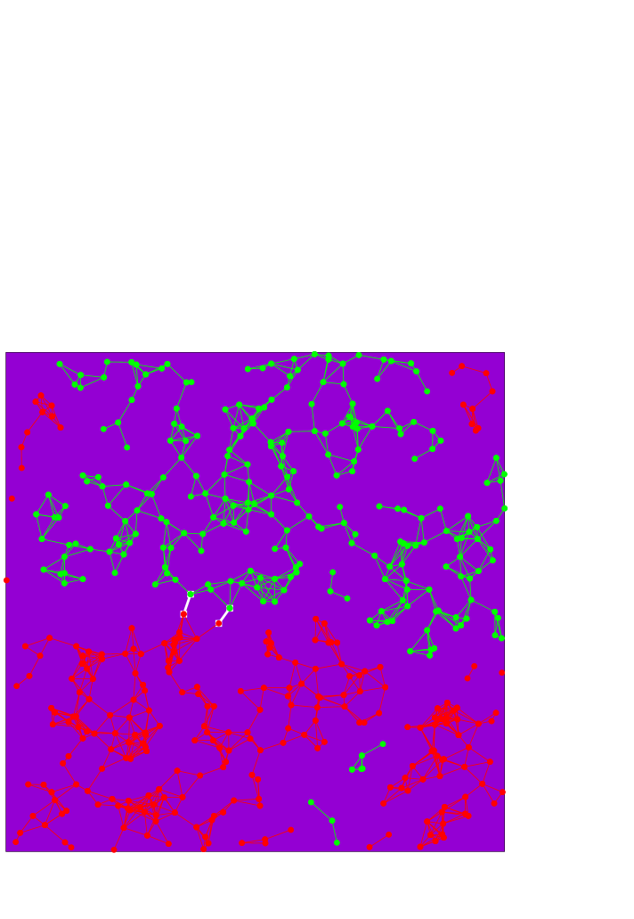
Figure 1: Optimal partition of an $N=500$ geometric graph with $C=5$. Any two points in the unit square are connected by an edge if their separating distance $d$ satisfies $N\pi d^{2}<5$. The 250 green points make up one subset, and the 250 red points make up the other. Over a sample of 30 runs, extremal optimization averaged a cutsize of 3.7, and eight times found partitions with a cutsize of 2 (shown here in white).

In graph (bi-)partitioning, we are given a set of $N$ points, where $N$ is even, and “edges” connecting certain pairs of points. The problem is to find a way of partitioning the points in two equal subsets, each of size $N/2$, with a minimal number of edges cutting across the partition (minimum “cutsize”). These points, for instance, could be positioned randomly in the unit square. A “geometric” graph of average connectivity $C$ would then be formed by connecting any two points within Euclidean distance $d$, where $N\pi d^{2}=C$ (see Fig. 1). Constraining the partitioned subsets to be of fixed (equal) size makes the solution to this problem particularly difficult. This geometric problem resembles those found in VLSI design, concerning the optimal partitioning of gates between integrated circuits VLSI .

Graph partitioning is an NP-hard optimization problem GareyJohnson : it is believed that for large $N$ the number of steps necessary for an algorithm to find the exact optimum must, in general, grow faster than any polynomial in $N$. In practice, however, the goal is usually to find near-optimal solutions quickly. Special-purpose heuristics to find approximate solutions to specific NP-hard problems abound AK ; JohnsonTSP . Alternatively, general-purpose optimization approaches based on stochastic procedures have been proposed Reeves ; Osman . The most widely applied of these have been physically motivated methods such as simulated annealing SA1 ; SA2 and genetic algorithms GA ; Bounds . These procedures, although slower, are applicable to problems for which no specialized heuristic exists. EO falls into the latter category, adaptable to a wide range of combinatorial optimization problems rather than crafted for a specific application.

Let us illustrate the general form of the EO algorithm by way of the explicit case of graph bi-partitioning. In close analogy to the Bak-Sneppen model of SOC BS , the EO algorithm proceeds as follows:

1. Choose an initial state of the system at will. In the case of graph partitioning, this means we choose an initial partition of the $N$ points into two equal subsets.

2. Rank each variable $i$ of the system according to its fitness value $\lambda_{i}$. For graph partitioning, the variables are the $N$ points, and we define $\lambda_{i}$ as follows: $\lambda_{i}=g_{i}/(g_{i}+b_{i})$, where $g_{i}$ is the number of (good) edges connecting $i$ to points within the same subset, and $b_{i}$ is the number of (bad) edges connecting $i$ to the other subset. [If point $i$ has no connections at all ($g_{i}=b_{i}=0$), let $\lambda_{i}=1$.]

3. Pick the least fit variable, i.e. the variable with the smallest $\lambda_{i}\in[0,1]$, and update it according to some move class. For graph partitioning, the move class is as follows: the least fit point (from either subset) is interchanged with a random point from the other subset, so that each point ends up in the opposite subset from where it started.

4. Repeat at (2) for a preset number of times. For graph partitioning we require $O(N)$ updates.

The result of an EO run is defined as the best (minimum cutsize) configuration seen so far. All that is necessary to keep track of, then, is the current configuration and the best so far in each run.

EO, like simulated annealing (SA) and genetic algorithms (GA), is inspired by observations of systems in nature. However, SA emulates the behavior of frustrated physical systems in thermal equilibrium: if one couples such a system to a heat bath of adjustable temperature, by cooling the system slowly one may come close to attaining a state of minimal energy. SA accepts or rejects local changes to a configuration according to the Metropolis algorithm MRRTT at a given temperature, enforcing equilibrium dynamics (“detailed balance”) and requiring a carefully tuned “temperature schedule”. In contrast, EO takes the system far from equilibrium: it applies no decision criteria, and all new configurations are accepted indiscriminately. It may appear that EO’s results would resemble an ineffective random search. But in fact, by persistent selection against the worst fitnesses, one quickly approaches near-optimal solutions. The contrast between EO and genetic algorithms (GA) is equally pronounced. GAs keep track of entire “gene pools” of states from which to select and “breed” an improved generation of solutions. EO, on the other hand, operates only with local updates on a single copy of the system, with improvements achieved instead by elimination of the bad.

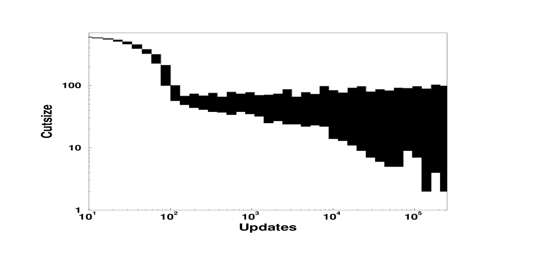
Figure 2: Evolution of the cutsize during an extremal optimization run on the $N=500$ geometric graph with $C=5$ (see Fig. 1). The shaded area marks the range of cutsizes explored in the respective time bins. The best cutsize ever found is 2, which is visited repeatedly in this run. In contrast to simulated annealing, which has large fluctuations in early stages of the run and then converges much later, extremal optimization quickly approaches a stage where broadly distributed fluctuations allow it to probe many local optima. In this run, a random initial partition was used, and the runtime on a 200MHz Pentium was 9sec.

Another important contrast to note is between EO and more conventional “greedy” update strategies. Methods such as greedy local search Osman successively update variables so that at each step, the solution is improved. This inevitably results in the system getting stuck in a local optimum, where no further improvements are possible. EO, while registering its greatest improvements towards the beginning of the run, nevertheless exhibits significant fluctuations throughout, as shown in Fig. 2. The result is that, even at late run-times, EO is able to cross sizable barriers and access new regions in configuration space.

There is a closer resemblance between EO and algorithms such as GSAT (for satisfiability) that choose, at each update step, the move resulting in the best subsequent outcome — whether or not that outcome is an improvement over the current solution GSAT . Also, versions of SA have been proposed Greene ; Reeves that enforce equilibrium dynamics by ranking local moves according to anticipated outcome, and then choosing them probabilistically. Similarly, Tabu Search Glover ; Reeves uses a greedy mechanism based on a ranking of the anticipated outcome of moves. But EO, significantly, makes moves using a fitness that is based not on anticipated outcome but purely on the current state of each variable.

Figs. 3a-b show that the results of EO rival those of a sophisticated SA algorithm developed for graph partitioning Johnson . Further improvements may be obtained from a slight modification to the EO procedure. Step (2) of the algorithm establishes a fitness rank for all points, going from rank $n=1$ for the worst to rank $n=N$ for the best fitness $\lambda$. (For points with degenerate values of $\lambda$, the ranks may be assigned in random order.) Now relax step (3) so that the points to be interchanged are both chosen stochastically, from a probability distribution over the rank order. This is done in the following way. Pick a point having rank $n$ with probability $P(n)\propto n^{-\tau},\leavevmode\nobreak\ 1\leq n\leq N$. Then pick a second point using the same process, though restricting ourselves this time to candidates from the opposite subset. The choice of a power-law distribution for $P(n)$ ensures that no regime of fitness gets excluded from further evolution, since $P(n)$ varies in a gradual, scale-free manner over rank. Universally, for a wide range of graphs, we obtain best results for $\tau\approx 1.2-1.6$. Fig. 3c shows these results for $\tau=1.5$, demonstrating its superior performance over both SA and the basic EO method.

What is the physical meaning of an optimal value for $\tau$? If $\tau$ is too small, we often dislodge already well-adapted points of high rank: “good” results get destroyed too frequently and the progress of the search becomes undirected. On the other hand, if $\tau$ is too large, the process approaches a deterministic local search (only swapping the lowest-ranked point from each subset) and gets stuck near a local optimum of poor quality. At the optimal value of $\tau$, the more fit variables of the solution are allowed to survive, without the search being too narrow. Our numerical studies have indicated that the best choice for $\tau$ is closely related to a transition from ergodic to non-ergodic behavior, with optimal performance of EO obtained near the edge of ergodicity. This will be the subject of future investigation.

To evaluate EO, we applied the algorithm to a testbed of graphs discussed in Refs. Johnson ; HL ; BM ; MF1 ; MF2 . The first set of graphs, originally introduced in Ref. Johnson , consists of eight geometric and eight “random” graphs. The geometric graphs in the testbed, labeled “U$N.C$”, are of sizes $N=500$ and 1000 and connectivities $C=5$, 10, 20 and 40. In a random graph, points are not related by a metric. Instead, any two points are connected with probability $p$, leading to an average connectivity $C\approx pN$. The random graphs in the testbed, labeled “G$Np$”, are of sizes $N=500$ and 1000 and connectivities $pN=2.5$, 5, 10 and 20. The best results reported to date on these graphs have been obtained from finely-tuned GA implementations BM ; MF1 ; MF2 . EO reproduces most of these cutsizes, and often at a fraction of the runtime, using $\tau=1.4$ and 30 runs of $200N$ update steps each. Comparative results are given in the upper half of Table 1.

Table 1: Best cutsizes (and total allowed runtime) for our testbed of graphs. Geometric graphs are labeled “U$N.C$”, and random graphs are labeled “G$Np$” where $C\approx pN$. GA results are the best reported in Ref. MF1 ; MF2 , using a 300MHz Pentium. SA and EO results are from our runs (SA parameters as determined in Ref. Johnson ), using a 200MHz Pentium. Comparison data for three of the large graphs are due to results from heuristics in Ref. HL , using a 50MHz Sparc20.

Geom. Graph	GA		SA		EO		Rand. Graph	GA		SA		EO
U500.5	2	(13s)	4	(3s)	2	(4s)	G500.005	49	(60s)	51	(5s)	51	(3s)
U500.10	26	(10s)	26	(2s)	26	(5s)	G500.01	218	(60s)	219	(4s)	218	(4s)
U500.20	178	(26s)	178	(1s)	178	(9s)	G500.02	626	(60s)	628	(3s)	626	(6s)
U500.40	412	(9s)	412	(.5s)	412	(16s)	G500.04	1744	(60s)	1744	(3s)	1744	(10s)
U1000.5	1	(43s)	3	(5s)	1	(8s)	G1000.0025	93	(120s)	102	(9s)	95	(6s)
U1000.10	39	(20s)	39	(3s)	39	(11s)	G1000.005	445	(120s)	451	(8s)	447	(8s)
U1000.20	222	(37s)	222	(2s)	222	(18s)	G1000.01	1362	(120s)	1366	(6s)	1362	(12s)
U1000.40	737	(38s)	737	(1s)	737	(33s)	G1000.02	3382	(120s)	3386	(6s)	3383	(20s)
Large Graph	GA		Ref. HL		EO		Large Graph			SA		EO
Hammond	90	(1s)	97	(8s)	90	(42s)	Nasa1824			739	(3s)	739	(6s)
($N=4720$; $C=5.8$)							($N=1824$; $C=20.5$)
Barth5	139	(44s)	146	(28s)	139	(64s)	Nasa2146			870	(2s)	870	(10s)
($N=15606$; $C=5.8$)							($N=2146$; $C=32.7$)
Brack2	731	(255s)	—		731	(12s)	Nasa4704			1292	(13s)	1292	(15s)
($N=62632$; $C=11.7$)							($N=4704$; $C=21.3$)
Ocean	464	(1200s)	499	(38s)	464	(200s)	Stufe10			371	(200s)	51	(180s)
($N=143437$; $C=5.7$)							($N=24010$; $C=3.8$)

The next set of graphs in our testbed are of larger size (up to $N=143$,437). The lower half of Table 1 summarizes EO’s results on these graphs, again using $\tau=1.4$ and 30 runs. On each graph, we used as many update steps as appeared productive for EO to reliably obtain stable results. This varied with the particularities of each graph, from $2N$ to $200N$ (further discussed below), and the reported runtimes are of course influenced by this. On the first four of the large graphs, the best results to date are once again due to GAs MF2 . EO reproduces all of these cutsizes, displaying an increasing runtime advantage as $N$ increases. SA’s performance on the graphs is extremely poor (comparable to its performance on Stufe10, shown later); we therefore substitute more competitive results given in Ref. HL using a variety of specialized heuristics. EO significantly improves upon these heuristics’ results, though at longer runtimes. On the final four graphs, for which no GA results were available, EO matches or dramatically improves upon SA’s cutsizes. And although the results from the U$N.C$ and G$Np$ graphs suggest that increasing $C$ slows down EO and speeds up SA, these results demonstrate that EO’s runtime is still nearly competitive with SA’s on the high-connectivity Nasa graphs.

Several factors account for EO’s speed. First of all, we employ a simple “greedy” start to construct the initial partition in step (1), as follows: pick a point at random, assigning it to one partition, then take all the points to which it connects, all the points to which those new points connect, and so on, assigning them all to the same partition. When no more connected points are available, construct the opposite partition by the same means, starting from a new random (unassigned) point. Alternate in this way, assigning new points to one or the other partition, until either one contains $N/2$ points. This clustering of connected points helps EO converge rapidly, and instantly eliminates from the running many trivial cases with zero cutsize. The procedure is most advantageous for smaller graphs, where it provides a significant speed-up; that speed-up becomes less relevant for larger graphs, but can still be productive if the graph has a distinct non-random structure (this was notably the case for Brack2). By contrast, greedy initialization does little to improve SA: unless the starting temperature is carefully fine-tuned, any initial advantage is quickly lost in randomization.

Second of all, we use an approximate sorting process in step (2) to accelerate the algorithm. At each update step, instead of perfectly ordering the fitnesses $\lambda_{i}$ (with runtime factor $CN\log{N}$), we arrange them on an ordered binary tree called a “heap”. The highest level, $l=0$, of this heap is the root of the tree and consists solely of the poorest fitness. All other fitnesses are placed below the root such that a fitness value at the level $l$ is connected in the tree to a single poorer fitness at level $l-1$, and to two better fitnesses at level $l+1$. Due to the binary nature of the tree, each level has exactly $2^{l}$ entries, except for the lowest level $l=[log_{2}N]$. We select a level $l$, $0\leq l\leq[log_{2}N]$, according to a probability distribution $Q(l)\sim 2^{-(\tau-1)l}$ and choose one of its $2^{l}$ entries with equal probability. The rank $n$ distribution of fitnesses thus chosen from the heap roughly approximates the desired function $P(n)\sim n^{-\tau}$ for a perfectly ordered list. The process of resorting the fitnesses in the heap introduces a runtime factor of only $C\log{N}$ per update step.

A further contributor to EO’s speed is the significantly smaller number of update steps (Fig. 2) that EO requires compared to, say, a complete SA temperature schedule. The quality of our large $N$ results confirms that $O(N)$ update steps are indeed sufficient for convergence. Generally, $200N$ steps were used per run, though in the case of the Nasa graphs only $30N$ steps were required for EO to reach its best results, and in the case of the Brack2 graph no more than $2N$ steps were necessary.

In summary, EO appears to be quite successful over a large variety of graphs. By comparison, GAs must be finely tuned for each type of graph in order to be successful, and SA is only useful for highly-connected graphs; Ref. EOperc demonstrates the dramatic advantage of EO over SA for sparse graphs. It is worth noting, though, that EO’s average performance has been varied. While on every graph, the best-found result was obtained at least twice in the 30 runs, the cutsizes obtained in other runs ranged from a 1% excess over the best (on the random graphs) to a 100% excess or far more (on the others). For instance, half of the Brack2 runs returned cutsizes near 731, but the other half returned cutsizes of above $2000$. This may be a product of an unusual structure in this particular graph, as noted in the discussion above on the initial partition construction. However, we hope that further insights into EO’s performance will be able to explain these wide fluctuations.

It is also clear that the EO algorithm is applicable to a wide range of combinatorial optimization problems involving a cost function. An example well known to computer scientists is the problem of maximum satisfiability. Since one must assign Boolean variables so as to maximize the number of satisfied clauses, a logical definition of fitness $\lambda_{i}$ for a variable $i$ is simply the satisfied fraction of clauses in which that variable appears. Another related problem of great physical interest is the spin-glass MPV , where spin variables $\sigma_{i}=\pm 1$ on a lattice are connected via a fixed (“quenched”) network of bonds $J_{ij}$ randomly assigned values of $+1$ or $-1$ when $i$ and $j$ are nearest neighbors (and 0 otherwise). In this system the variables $\sigma_{i}$ try to minimize the energy represented by the Hamiltonian $H=-\sum_{i,j}J_{ij}\sigma_{i}\sigma_{j}$. It is intuitive that the fitness associated with each lattice site here is the local energy contribution, $\lambda_{i}={1\over 2}\sigma_{i}\sum_{j}J_{ij}\sigma_{j}$. These applications of EO have the conceptual advantage that no global constraint needs to be satisfied, so that on each update a single variable can be chosen according to $P(n)\sim n^{-\tau}$; that variable undergoes a unambiguous flip, affecting the fitnesses of all its neighbors. We are currently investigating these problems.

In such cases, where the cost can be phrased in terms of a spin Hamiltonian MPV , the implementation of EO is particularly straightforward. The concept of fitness, however, is equally meaningful in any discrete optimization problem whose cost function can be decomposed into $N$ equivalent degrees of freedom. Thus, EO may be applied to many other NP-hard problems, even those where the choice of quantities for the fitness function, as well as the choice of elementary move, is less than obvious. One good example of this is the traveling salesman problem. Even so, we find there that EO presents a challenge to more finely tuned methods.

In the traveling salesman problem (TSP), $N$ points (“cities”) are given, and every pair of cities $i$ and $j$ is separated by a distance $d_{ij}$. The problem is to connect the cities using the shortest closed “tour”, passing through each city exactly once. For our purposes, take the $N\times N$ distance matrix $d_{ij}$ to be symmetric. Its entries could be the Euclidean distances between cities in a plane — or alternatively, random numbers drawn from some distribution, making the problem non-Euclidean. (The former case might correspond to a business traveler trying to minimize driving time; the latter to a traveler trying to minimize expenses on a string of airline flights, whose prices certainly do not obey triangle inequalities!)

For the TSP, we implement EO in the following way. Consider each city $i$ as a degree of freedom, with a fitness based on the two links emerging from it. Ideally, a city would want to be connected to its first and second nearest neighbor, but is often “frustrated” by the competition of other cities, causing it to be connected instead to (say) its $\alpha$th and $\beta$th neighbors, $1\leq\alpha,\beta\leq N-1$. Let us define the fitness of city $i$ to be $\lambda_{i}=3/(\alpha_{i}+\beta_{i})$, so that $\lambda_{i}=1$ in the ideal case.

Defining a move class (step (3) in EO’s algorithm) is more difficult for the TSP than for graph partitioning, since the constraint of a closed tour requires an update procedure that changes several links at once. One possibility, used by SA among other local search methods, is a “two-change” rearrangement of a pair of non-adjacent segments in an existing tour. There are $O(N^{2})$ possible choices for a two-change. Most of these, however, lead to even worse results. For EO, it would not be sufficient to select two independent cities of poor fitness from the rank list, as the resulting two-change would destroy more good links than it creates. Instead, let us select one city $i$ according to its fitness rank $n_{i}$, using the distribution $P(n)\sim n^{-\tau}$ as before, and eliminate the longer of the two links emerging from it. Then, reconnect $i$ to a close neighbor, using the same distribution function $P(n)$ as for the rank list of fitnesses, but now applied instead to a rank list of $i$’s neighbors ($n=1$ for nearest neighbor, $n=2$ for second-nearest neighbor, and so on). Finally, to form a valid closed tour, one link from the new city must be replaced; there is a unique way of doing so. For the optimal choice of $\tau$, this move class allows us the opportunity to produce many good neighborhood connections, while maintaining enough fluctuations to explore the configuration space.

We performed simulations at $N=16$, 32, 64, 128 and 256, in each case generating ten random instances for both the Euclidean and non-Euclidean TSP. The Euclidean case consisted of $N$ points placed at random in the unit square with periodic boundary conditions; the non-Euclidean case consisted of a symmetric $N\times N$ distance matrix with elements drawn randomly from a uniform distribution on the unit interval. On each instance we ran both EO and SA from random initial conditions, selecting for both methods the best of 10 runs. EO used $\tau=4$ (Eucl.) and $\tau=4.4$ (non-Eucl.), with $16N^{2}$ update steps. SA used an annealing schedule with $\Delta T/T=0.9$ and temperature length $32N^{2}$. These parameters were chosen to give EO and SA virtually equal runtimes. The results of the runs are given in Table 2, along with baseline results using an exact algorithm exact .

Table 2: Best tour-lengths found for the Euclidean and the random-distance TSP. Results for each value of $N$ are averaged over 10 instances, using on each instance an exact algorithm (except for $N=256$ Euclidean where none was available), the best-of-ten EO runs and the best-of-ten SA runs. Euclidean tour-lengths are rescaled by $1/\sqrt{N}$.

$N$	Exact	EO10	SA10
Euclidean:  16	0.71453	0.71453	0.71453
32	0.72185	0.72237	0.72185
64	0.72476	0.72749	0.72648
128	0.72024	0.72792	0.72395
256	—	0.72707	0.71854
Random Distance:  16	1.9368	1.9368	1.9368
32	2.1941	2.1989	2.1953
64	2.0771	2.0915	2.1656
128	2.0097	2.0728	2.3451
256	2.0625	2.1912	2.7803

While the EO results trail those of SA by up to about 1% in the Euclidean case, EO significantly outperforms SA for the non-Euclidean (random distance) TSP. This may be due to the substantial configuration space energy barriers exhibited in non-Euclidean instances; equilibrium methods such as SA get trapped by these barriers, whereas non-equilibrium methods such as EO do not. (Interestingly, SA’s performance here diminishes rather than improves when runtimes are increased by using longer temperature schedules!) For Euclidean instances, the tour lengths found by EO on single runs were at worst 1% over the best-of-ten, and the tour lengths found by SA were at worst 4% over the best-of-ten; for non-Euclidean instances, these worst excesses were 5% (EO) and 10% (SA). Finally, note that one would not expect a general method such as EO to be competitive here with the more specialized optimization algorithms, such as Iterated Lin-Kernighan CLO ; JohnsonILK , designed particularly with the TSP in mind. But remarkably, EO’s performance in both the Euclidean and non-Euclidean cases — within several percent of optimality for $N\leq 256$ — places it not far behind the leading specially-crafted TSP heuristics JohnsonTSP .

Our results therefore indicate that a simple extremal optimization approach based on self-organizing dynamics can often outperform state-of-the-art (and far more complicated or finely tuned) general-purpose algorithms, such as simulated annealing or genetic algorithms, on hard optimization problems. Based on its success on the generic and broadly applicable graph partitioning problem, as well as on the TSP, we believe the concept will be applicable to numerous other NP-hard problems. It is worth stressing that the rank ordering approach employed by EO is inherently non-equilibrium. Such an approach could not, for instance, be used to enhance SA, whose temperature schedule requires equilibrium conditions. This rank ordering serves as a sort of “memory”, allowing EO to retain well-adapted pieces of a solution. In this respect it mirrors one of the crucial properties noted in the Bak-Sneppen model PRE96 ; PRL97 . At the same time, EO maintains enough flexibility to explore further reaches of the configuration space and to “change its mind”. Its success at this complex task provides motivation for the use of extremal dynamics to model mechanisms such as learning, as has been suggested recently to explain the high degree of adaptation observed in the brain bakbrain .

Thanks to D. S. Johnson and O. Martin for their helpful remarks.

Figure 3: Comparison of 1000-run trials using various optimization methods on $N=500$ random graph with $pN=5$. The histograms give, for each method, the frequency with which a particular cutsize has been obtained during the trial runs. (A) shows the performance of simulated annealing, reproducing results given in Ref. Johnson . (B) shows the results for the basic implementation of extremal optimization. (C) shows the results for extremal optimization using a probability distribution with $\tau=1.5$. The best cutsize ever found for this graph is 206. This result appeared only once over the 1000 simulated annealing runs, but occurred 80 times over the 1000 extremal optimization runs at $\tau=1.5$.

References

- (1) C. Darwin, The Origin of Species by Means of Natural Selection (Murray, London, 1859).
- (2) P. Bak, C. Tang and K. Wiesenfeld, Self-organized criticality: an explanation of -noise, Phys. Rev. Lett. 59 (1987) 381–384.
- (3) P. Bak, How Nature Works (Springer, New York, 1996).
- (4) M. Paczuski, S. Maslov and P. Bak, Avalanche dynamics in evolution, growth, and depinning models, Phys. Rev. E 53 (1996) 414–443.
- (5) P. Bak and K. Sneppen, Punctuated equilibrium and criticality in a simple model of evolution, Phys. Rev. Lett. 71 (1993) 4083–4086.
- (6) K. Sneppen, P. Bak, H. Flyvbjerg and M.H. Jensen, Evolution as a self-organized critical phenomenon, Proc. Natl. Acad. Sci. 92 (1995) 5209–5213.
- (7) S. Boettcher and A. G. Percus, Extremal Optimization: Methods derived from Co-Evolution, GECCO-99: Proceedings of the Genetic and Evolutionary Computation Conference (Morgan Kaufmann, San Francisco, 1999), 825–832.
- (8) A.E. Dunlop and B.W. Kernighan, A procedure for placement of standard-cell VLSI circuits, IEEE Trans. on Computer-Aided Design CAD–4 (1985) 92–98.
- (9) M.R. Garey and D.S. Johnson, Computers and Intractability: A Guide to the Theory of NP-Completeness (Freeman, New York, 1979).
- (10) C.J. Alpert and A.B. Kahng, Recent directions in netlist partitioning: a survey, Integration: the VLSI Journal 19 (1995) 1–81.
- (11) D.S. Johnson and L.A. McGeoch, The traveling salesman problem: a case study, in: E.H.L. Aarts and J.K. Lenstra, eds., Local Search in Combinatorial Optimization (Wiley, New York, 1997) 215–310.
- (12) Modern Heuristic Techniques for Combinatorial Problems, Ed. C. R. Reeves (Wiley, New York, 1993).
- (13) Meta-Heuristics: Theory and Application, Eds. I. H. Osman and J. P. Kelly (Kluwer, Boston, 1996).
- (14) S. Kirkpatrick, C.D. Gelatt and M.P. Vecchi, Optimization by simulated annealing, Science 220 (1983) 671–680.
- (15) V. Černy, A thermodynamical approach to the traveling salesman problem: an efficient simulation algorithm, J. Optimization Theory Appl. 45 (1985) 41–51.
- (16) J. Holland, Adaptation in Natural and Artificial Systems (University of Michigan Press, Ann Arbor, 1975).
- (17) D.G. Bounds, New optimization methods from physics and biology, Nature 329 (1987) 215–219.
- (18) N. Metropolis, A.W. Rosenbluth, M.N. Rosenbluth, A.H. Teller and E. Teller, Equation of state calculations by fast computing machines, J. Chem. Phys. 21 (1953) 1087–1092.
- (19) B. Selman, D. Mitchell and H. Levesque, A new method for solving hard satisfiability problems, Proc. AAAI–92, San Jose, CA (1995) 440–446.
- (20) J.W. Greene and K.J. Supowit, Simulated Annealing without rejected moves, IEEE Trans. on Computer-Aided Design CAD–5 (1986) 221–228.
- (21) F. Glover, Future paths for integer programming and links to artificial intelligence, Computers & Ops. Res. 13 (1986) 533–549.
- (22) D.S. Johnson, C.R. Aragon, L.A. McGeoch and C. Schevon, Optimization by simulated annealing: an experimental evaluation, part I (graph partitioning), Operations Research 37 (1989) 865–892.
- (23) B.A. Hendrickson and R. Leland, A multilevel algorithm for partitioning graphs, in: Proceedings Supercomputing ’95, San Diego, CA (1995).
- (24) T.N. Bui and B.R. Moon, Genetic algorithm and graph partitioning, IEEE Trans. on Computers 45 (1996) 841–855.
- (25) P. Merz and B. Freisleben, Memetic algorithms and the fitness landscape of the graph bi-partitioning problem, in: A.E. Eiben, T. Bäck, M. Schoenauer and H.-P. Schwefel, eds., Lecture Notes in Computer Science: Parallel Problem Solving From Nature — PPSN V (Springer, Berlin, 1998), v. 1498, 765–774.
-
(26)
P. Merz and B. Freisleben, Fitness landscapes, memetic algorithms and
greedy operators for graph bi-partitioning, Technical Report No. TR–98–01, Department of Electrical Engineering and Computer Science,
University of Siegen, Germany (1998), available at:
http://www.informatik.uni-siegen.de/~pmerz/publications.html. - (27) S. Boettcher, Extremal Optimization of Graph Partitioning at the Percolation Threshold, J. Phys. A: Math. Gen. 32 (1999) 5201–5211.
- (28) M. Mezard, G. Parisi, and M. A. Virasoro, Spin Glass Theory and Beyond (World Scientific, Singapore, 1987).
-
(29)
C. Hurwitz, GNU tsp_solve, available at:
http://www.cs.sunysb.edu/~algorith/implement/tsp/implement.shtml. - (30) O.C. Martin and S.W. Otto, Combining simulated annealing with local search heuristics, Annals of Operations Research 63 (1996) 57–75.
- (31) D.S. Johnson, Local optimization and the traveling salesman problem, in: M.S. Paterson, ed., Lecture Notes in Computer Science: Automata, Languages and Programming (Springer, Berlin, 1990), v. 443, 446–461.
- (32) S. Boettcher and M. Paczuski, Ultrametricity and memory in a solvable model of self-organized criticality, Phys. Rev. E 54 (1996) 1082–1095.
- (33) S. Boettcher and M. Paczuski, Aging in a model of self-organized criticality, Phys. Rev. Lett. 79 (1997) 889–892.
- (34) D.R. Chialvo and P. Bak, Learning from mistakes, Neuroscience 90 (19990 1137–1148.