Can we Measure Superflow on Quenching ${}^{4}He$?

Abstract

Zurek has provided a simple picture for the onset of the $\lambda$-transition in ${}^{4}He$, not currently supported by vortex density experiments. However, we argue that the seemingly similar argument by Zurek that superflow in an annulus of ${}^{4}He$ at a quench will be measurable is still valid.

As the early universe cooled it underwent a series of phase transitions, whose inhomogeneities have observable consequences. To understand how such transitions occur it is necessary to go beyond the methods of equilibrium thermal field theory that identified the transitions in the first instance.

In practice, we often know remarkably little about the dynamics of quantum field theories. A simple question to ask is the following: In principle, the field correlation length diverges at a continuous transition. In reality, it does not. What happens? Using simple causal arguments Kibble[1, 2] made estimates of this early field ordering, because of the implications for astrophysics.

There are great difficulties in converting predictions for the early universe into experimental observations. Zurek suggested[3] that similar arguments were applicable to condensed matter systems for which direct experiments could be performed. In particular, for ${}^{4}He$ he argued that the measurement of superflow at a quench provided a simple test of these ideas. We present a brief summary of his argument.

Assume that the dynamics of the ${}^{4}He$ lambda-transition can be derived from an explicitly time-dependent Landau-Ginzburg free energy of the form

$$F(T)=\int d^{3}x\,\,\bigg{(}\frac{\hbar^{2}}{2m}|\nabla\phi|^{2}+\alpha(T)|\phi|^{2}+\frac{1}{4}\beta|\phi|^{4}\bigg{)},$$ (1)

in which $\alpha(T)$ vanishes at the critical temperature $T_{c}$. Explicitly, let us assume the mean-field result $\alpha(T)=\alpha_{0}\epsilon(T_{c})$, where $\epsilon=(T/T_{c}-1)$, remains valid as $T/T_{c}$ varies with time $t$. In particular, we first take $\alpha(t)=\alpha(T(t))=-\alpha_{0}t/\tau_{Q}$ in the vicinity of $T_{c}$. Then the fundamental length and time scales $\xi_{0}$ and $t_{0}$ are given from Eq.1 as $\xi_{0}^{2}=\hbar^{2}/2m\alpha_{0}$ and $\tau_{0}=\hbar/\alpha_{0}$. It follows that the equilibrium correlation length $\xi_{eq}(t)=\xi_{eq}(T(t))$ and the relaxation time $\tau(t)$ diverge at $T_{c}$, which we take to be when $t$ vanishes, as

$$\xi_{eq}(t)=\xi_{0}\bigg{|}\frac{t}{\tau_{Q}}\bigg{|}^{-1/2},\,\,\tau(t)=\tau_{0}\bigg{|}\frac{t}{\tau_{Q}}\bigg{|}^{-1}.$$ (2)

Although $\xi_{eq}(t)$ diverges at $t=0$ this is not the case for the true correlation length $\xi(t)$, which can only grow so far in a finite time. Initially, for $t<0$, when we are far from the transition, we can assume that the field correlation length $\xi(t)$ tracks $\xi_{eq}(t)$ approximately. However, as we get closer to the transition $\xi_{eq}(t)$ begins to increase arbitrarily fast. As a crude upper bound, the true correlation length fails to keep up with $\xi_{eq}(t)$ by the time $-{\bar{t}}$ at which $\xi_{eq}$ is growing at the speed of sound $c(t)=\xi_{eq}(t)/\tau(t)$, which determines the rate at which the order-parameter can change. The condition $d\xi_{eq}(t)/dt=c(t)$ is satisfied at $t=-{\bar{t}}$, where ${\bar{t}}=\sqrt{\tau_{Q}\tau_{0}}$, with corresponding correlation length

$${\bar{\xi}}=\xi_{eq}(-{\bar{t}})=\xi_{0}\bigg{(}\frac{\tau_{Q}}{\tau_{0}}\bigg{)}^{1/4}.$$ (3)

After this time it is assumed that the relaxation time is so long that $\xi(t)$ is essentially frozen in at ${\bar{\xi}}$ until time $t\approx+{\bar{t}}$, when it sets the scale for the onset of the broken phase.

A concrete realisation of how the freezing sets in is provided by the time-dependent Landau-Ginzburg (TDLG) equation for $F$ of (1)[4],

$$\frac{1}{\Gamma}\frac{\partial\phi_{a}}{\partial t}=-\frac{\delta F}{\delta\phi_{a}}+\eta_{a},$$ (4)

for $\phi=(\phi_{1}+i\phi_{2})/\sqrt{2}$, where $\eta_{a}$ is Gaussian noise. We can show self-consistently[5] that, for the relevant time-interval $-{\bar{t}}\leq t\leq{\bar{t}}$ the self-interaction term can be neglected ($\beta=0$), whereby a simple calculation finds $\xi\approx{\bar{\xi}}$ in this interval, as predicted. It thus happens that, at the onset of the phase transition, the field fluctuations are approximately Gaussian. The field phases $e^{i\theta({\bf r})}$, where $\phi({\bf r})=|\phi({\bf r})|e^{i\theta({\bf r})}$, are then correlated on the same scale as the fields.

Consider a closed path in the bulk superfluid with circumference $C\gg\xi(t)$. Naively, the number of ’regions’ through which this path passes in which the phase is correlated is ${\cal N}=O(C/\xi(t))$. Assuming an independent choice of phase in each ’region’, the r.m.s phase difference along the path is

$$\Delta\theta_{C}\approx\sqrt{{\cal N}}=O(\sqrt{C/\xi(t)}).$$ (5)

If we now consider a quench in an annular container of similar circumference $C$ of superfluid ${}^{4}He$ and radius $l\ll C$, Zurek suggested that the phase locked in is also given by Eq.5, with ${\bar{\xi}}$ of Eq.3. Since the phase gradient is directly proportional to the superflow velocity we expect a flow after the quench with r.m.s velocity

$$\Delta v=O\bigg{(}\frac{\hbar}{m}\sqrt{\frac{1}{C{\bar{\xi}}}}\bigg{)}.$$ (6)

provided $l=O({\bar{\xi}})$. Although in bulk fluid this superflow will disperse, if it is constrained to a narrow annulus it should persist, and although not large is measurable.

In addition to this experiment, Zurek also suggested that the same correlation length ${\bar{\xi}}$ should characterise the separation of vortices in a quench. In an earlier paper[5] one of us showed that this is too simple. Causality arguments are not enough, and whether vortices form on this scale is also determined by the thermal activation of the Ginzberg regime, in which all ${}^{4}He$ experiments take place. Experimentally, this seems to be the case[7].

Our aim in this paper is to see whether thermal fluctuations interfere with the prediction Eq.6, for which experiments have yet to be performed. Again consider a circular path in the bulk fluid (in the 1-2 plane), circumference $C$, the boundary of a surface $S$. For given field configurations $\phi_{a}({\bf x})$ the phase change $\theta_{C}$ along the path can be expressed as the surface integral

$$\theta_{C}=2\pi\int_{{\bf x}\in S}d^{2}x\,\,\rho({\bf x}),$$ (7)

where the topological density $\rho({\bf x})$ is given by

$$\rho({\bf x})=\delta^{2}[\phi({\bf x})]\epsilon_{jk}\partial_{j}\phi_{1}({\bf x})\partial_{k}\phi_{2}({\bf x}),\,\,\,i,j=1,2$$ (8)

where $\epsilon_{12}=-\epsilon_{21}=1$, otherwise zero.

The ensemble average $\langle\rho({\bf x})\rangle_{t}$ is taken to be zero at all times $t$, guaranteed by taking $\langle\phi_{a}({\bf x})\rangle_{t}=0=\langle\phi_{a}({\bf x})\partial_{j}\phi_{b}({\bf x})\rangle_{t}$. That is, we quench from an initial state with no rotation. For the Gaussian fluctuations that are relevant for the times of interest[5, 6], all correlations are given in terms of the diagonal equal-time correlation function $G(r,t)$, defined by

$$\langle\phi_{a}({\bf x})\phi_{b}({\bf 0})\rangle_{t}=\delta_{ab}G(r,t)\,\,\,\,\,r=|{\bf x}|.$$ (9)

The correlation length $\xi(t)$ is defined by $G(r,t)=o(e^{-r/\xi(t)})$, for large $r>\xi(t)$. The TDLG does not lead to simple exponential behaviour, but there is no difficulty in defining $\xi(t)$ in practice[5, 6].

The variance in the phase change around $C$, $\Delta\theta_{C}$ is determined from

$$(\Delta\theta_{C})^{2}=4\pi^{2}\int_{{\bf x}\in S}d^{2}x\int_{{\bf y}\in S}d^{2}y\,\langle\rho({\bf x})\rho({\bf y})\rangle_{t}.$$ (10)

The properties of densities for Gaussian fields have been studied in detail[8, 9]. Define $f(r,t)$ by $f(r,t)=G(r,t)/G(0,t)$. On using the conservation of charge

$$\int\,d^{2}x\,\langle\rho({\bf x})\rho({\bf 0})\rangle_{t}=0$$ (11)

it is not difficult to show, from the results of[8, 9], that $\Delta\theta_{C}$ satisfies

$$(\Delta\theta_{C})^{2}=-\int_{{\bf x}\not\in S}d^{2}x\int_{{\bf y}\in S}d^{2}y\,\,{\cal C}(|{\bf x}-{\bf y}|,t),$$ (12)

where ${\bf x}$ and ${\bf y}$ are in the plane of $S$, and

$${\cal C}(r,t)=\frac{1}{r}\frac{\partial}{\partial r}\bigg{(}\frac{f^{\prime 2}(r,t)}{1-f^{2}(r,t)}\bigg{)}.$$ (13)

Since $G(r,t)$ is short-ranged ${\cal C}(r,t)$ is short-ranged also. With ${\bf x}$ outside $S$, and ${\bf y}$ inside $S$, all the contribution to $(\Delta\theta_{C})^{2}$ comes from the vicinity of the boundary of $S$, rather than the whole area. That is, if we removed all fluid except for a strip from the neighbourhood of the contour $C$ we would still have the same result. This supports the assertion by Zurek that the correlation length for phase variation in bulk fluid is also appropriate for annular flow. The purpose of the annulus (more exactly, a circular capillary of circumference $C$ with radius $l\ll C$) is to stop this flow dissipating into the bulk fluid.

More precisely, suppose that $C\gg\xi(t)$. Then, if we take the width $2l$ of the strip around the contour to be larger than the correlation length of ${\cal C}(r,t)$, Eq.12 can be written as

$$(\Delta\theta_{C})^{2}\approx-2\,C\int_{0}^{\infty}dr\,r^{2}\,\,{\cal C}(r,t).$$ (14)

The linear dependence on $C$ is purely a result of Gaussian fluctuations.

Insofar as we can identify the bulk correlation with the annular correlation, instead of Eq.6, we have

$$\Delta v=\frac{\hbar}{m}\sqrt{\frac{1}{C\xi_{s}(t)}}.$$ (15)

The step length $\xi_{s}(t)$ is given by

$$\frac{1}{\xi_{s}(t)}=2\int_{0}^{\infty}dr\frac{f^{\prime 2}(r,t)}{1-f^{2}(r,t)}.$$ (16)

There are two important differences between Eq.15 and Eq.6. The first is in the choice of time for which $\Delta v$ of Eq.15 is to be evaluated. In Eq.6 the time is the time $-{\bar{t}}$ of freezing in of the field correlation. Since $\xi(t)$ does not change much in the interval $-{\bar{t}}<t<{\bar{t}}$ we can as well take $t=0$. We shall argue below that for Eq.15 a more appropriate time is the spinodal time $t_{sp}$ at which the transition has completed itself in the sense that the fields have begun to populate the ground states.

Secondly, a priori there is no reason to identify $\xi_{s}(t_{sp})$ with either ${\bar{\xi}}$ (or even $\xi(t_{sp})$). In particular, because ${\bar{\xi}}$ in Eq.6 is defined from the large-distance behaviour of $G(r,t)$, and thereby on the position of the nearest singularity of $G(k,t)$ in the $k$-plane, it does not depend on the scale at which we observe the fluid. This is not the case for $\xi_{s}(t)$ which, from Eq.16, explores all distance scales. Because of the fractal nature of the short wavelength fluctuations, $\xi_{s}(t)$ will depend on how many are included, i.e. the scale at which we look. If we quench in an annular capillary of radius $l$ much smaller than its circumference, we are, essentially, coarsegraining to that scale. That is, the observed variance in the flux along the annulus is $\pi l^{2}\Delta v$ for $\Delta v$ averaged on a scale $l$. We make the approximation that that is the major effect of quenching in an annulus. This cannot be wholly true, but it is plausible if the annulus is not too narrow for boundary effects to be important.

Provisionally we introduce a coarsegraining by hand, modifying $G(r,t)$ by damping short wavelengths $O(l)$ as

$$G(r,t;l)=\int d\!\!\!/^{3}k\,e^{i{\bf k}.{\bf x}}G(k,t)\,e^{-k^{2}l^{2}}.$$ (17)

We shall denote the value of $\xi_{s}$ obtained from Eq.17 as $\xi_{s}(t;l)$. It permits an expansion in terms of the moments of $G(k,t)\,e^{-k^{2}l^{2}}$,

$$G_{n}(t;l)=\int_{0}^{\infty}dk\,k^{2n}\,G(k,t)\,e^{-k^{2}l^{2}}.$$ (18)

For small $r$ it follows that $f^{\prime 2}(r,t;l)/(1-f^{2}(r,t;l))$

$$=\frac{G_{2}}{3G_{1}}\bigg{[}1-\bigg{(}\frac{3G_{3}}{20G_{2}}-\frac{G_{2}}{12G_{1}}\bigg{)}r^{2}+O(r^{4})\bigg{]}.$$ (19)

Although, for large $r$, $f^{\prime}(r,t;l)^{2}=o(e^{-2r/\xi(t)})$, we find that the bulk of the integral Eq.16 lies in the forward peak, and that a good upper bound for $\xi_{s}$ is given by just integrating the quadratic term, whence

$$\frac{1}{\xi_{s}(t;l)}\geq\frac{1}{\xi^{min}_{s}(t;l)}=\frac{4G_{2}}{9G_{1}}\bigg{(}\frac{3G_{3}}{20G_{2}}-\frac{G_{2}}{12G_{1}}\bigg{)}^{-1/2},$$ (20)

with the equality slightly overestimated. In units of $\xi_{0}$ and $\tau_{0}$ we have, in the linear regime[5],

$$G_{n}(t;l)\approx\frac{I_{n}}{2^{n+1/2}}\,e^{(t/{\bar{t}})^{2}}\int_{0}^{\infty}dt^{\prime}\,\frac{e^{-(t^{\prime}-t)^{2}/{\bar{t}}^{2}}}{[t^{\prime}+l^{2}/2]^{n+1/2}}\frac{T(t^{\prime})}{T_{c}},$$ (21)

where $I_{n}=\int_{0}dkk^{2n}\,e^{-k^{2}}$. The presence of the $T(t^{\prime})/T_{c}$ term is a reminder that the strength of the noise $\eta$ is proportional to temperature. However, for the time scales $O({\bar{t}})\ll\tau_{Q}$ of interest to us this ratio remains near to unity and we ignore it. For small relative times the integrand gets a large contribution from the ultraviolet cutoff dependent lower endpoint, increasing as $n$ increases.

If we return to the Landau-Ginzberg equation Eq.4 we find that $\langle|\phi|^{2}\rangle_{t}\ll\alpha_{0}/\beta$ in the interval ${-\bar{t}}\leq t\leq{\bar{t}}$. Although the field has frozen in, the fluctuations have amplitudes that are more or less uniform across all wavelengths. As a result, what we see depends totally on the scale at which we look. Specifically, from Eq.21 $\xi^{min}_{s}(0;l)=O(l)$, as shown in the lowest curve of Fig.1.

If, as suggested by Zurek, we take $l=O({\bar{\xi}})$ we recover Eq.6 qualitatively, although a wider bore would give a correspondingly smaller flow. However, this is not the time at which to look for superflow since, although the field correlation length $\xi(t)$ may have frozen in by $t=0$, the symmetry breaking has not begun.

Assuming the linearised[5] Eq.4 for small times $t>0$ we see that, as the unfreezing occurs, long wavelength modes with $k^{2}<t/\tau_{Q}$ grow exponentially and soon begin to dominate the correlation functions. How long a time we have depends on the self-coupling $\beta$ which, through $G_{1}$, sets the shortest time scale. This is because, at the absolute latest, $G_{1}$ must stop its exponential growth at $t=t_{sp}$, when $\langle|\phi|^{2}\rangle_{t_{sp}}$, satisfies $\langle|\phi|^{2}\rangle_{t_{sp}}=\alpha_{0}/\beta$. We further suppose that the effect of the backreaction that stops the growth initially freezes in any structure. In Fig.1 we also show $\xi^{min}_{s}(t;l)$ for $t=3{\bar{t}}$ and $t=4{\bar{t}}$, increasing as $t$ increases.

For ${}^{4}He$ with quenches of milliseconds the field magnitude has grown to its equilibrium value before the scale-dependence has stopped[5]. For vortex formation, for which the scale is $O(\xi_{0})$, the thickness of a vortex, the dependence of the density on scale makes the interpretation of observations problematic. This is not the same here. That the incoherent $\xi_{s}$ depends on radius $l$ is immaterial. The end result is that

$$\Delta v=\frac{\hbar}{m}\sqrt{\frac{1}{C\xi_{s}(t_{sp};l)}}.$$ (22)

We saw that the expression Eq.20 for $\xi_{s}$ assumed that $2l$ is larger than

$$\xi_{eff}(t;l)=\bigg{(}\frac{3G_{3}}{20G_{2}}-\frac{G_{2}}{12G_{1}}\bigg{)}^{-1/2}.$$ (23)

Otherwise the correlations in the bulk fluid from which we want to extract annular behaviour are of longer range than the annulus thickness. Numerically, we find that $\xi_{eff}(0,l)=2l$ very accurately at $t=0$, but that $\xi_{eff}(t,l)\geq 2l$ for all $t>0$. A crude way to accomodate this is to cut off the integral Eq.14. With a little effort, we see that the effect of this is that $\xi^{min}_{s}(t_{sp},l)$ of Eq.20 is replaced by

$$\xi^{max}_{s}(t_{sp},l)=\xi^{min}_{s}(t_{sp},l)[1-(1-4l^{2}/\xi_{eff}(t_{sp},l)^{2})^{3/2}]^{-1},$$ (24)

greater than $\xi^{min}_{s}(t_{sp},l)$ and thereby reducing the flow velocity for narrower annuli. These are the dashed curves in Fig.1. The effect is largest for small radii $l\leq{\bar{\xi}}$, for which the approximation of trying to read the behaviour of annular flow from bulk behaviour is most suspect. A more realistic approach for such narrow capillaries is to treat the system as one-dimensional[3]. For this reason we have only considered $l\geq{\bar{\xi}}$ in Fig.1. We would expect, from Eq.20, that $\xi_{s}(t_{sp};l)$ has an upper bound that lies somewhere between the curves.

Once $l$ is very large, so that the power in the fluctuations is distributed strongly across all wavelengths we recover our earlier result, that $\xi_{s}(t_{sp};l)=O(l)$. In Fig.1 this corresponds to the curves becoming parallel as $l$ increases for fixed $t$. However, the change is sufficiently slow that annuli, significantly wider than ${\bar{\xi}}$, for which experiments are more accessible, will give almost the same flow as narrower annuli. This would seem to extend the original Zurek prediction of Eq.6 to thicker annuli, despite our expectations for incoherent flow. However, we stress again that caution is necessary, since in the approximation to characterise an annulus by a coarse-grained ring without boundaries we have ignored effects in the direction perpendicular to the annulus. In particular, the circular cross-section of the tube has not been taken into account. One consequence of this is that infinite (non-selfintersecting) vortices in the bulk fluid have no counterpart in an annulus. Removing such strings will have an effect on $\Delta\theta_{C}$, since the typical fraction of vortices in infinite vortices is at the level of $70\%$. However, at the spinodal time the fluctuations in ${}^{4}He$ are relatively enhanced in the long wavelengths, and such an enhancement is known to reduce the amount of infinite vortices, perhaps to something nearer to $20\%$. The details of this effect (being pursued elsewhere) are unclear but, for the sake of argument we take the predictions of the curves in Fig.1 as a rough guide in the vicinity of their minima.

So far we have avoided the question as to which time curves we should follow. This is because $t_{sp}$ itself depends on the scale $l$ of the spatial volume for which the field average achieves its ground state value. In practice variation is small, with $t_{sp}$ for ${}^{4}He$ varying from about $3{\bar{t}}$ to $4{\bar{t}}$ as $l$ varies from $\xi_{0}\ll{\bar{\xi}}$ to $l=10{\bar{\xi}}$. Since the curves for $\xi_{s}(t_{sp};l)$ lie so close to one another in Fig.1 once $l\geq 4{\bar{\xi}}$ the scale at which the coarse-grained field begins to occupy the ground states becomes largely irrelevant.

Since $\Delta v$ only depends on $\xi_{s}^{-1/2}$ it is not sensitive to choice of $l>2{\bar{\xi}}$ at the relevant $t$. Given all these approximations our final estimate is (in the cm/sec units of Zurek[3])

$$\Delta v\approx 0.2(\tau_{Q}[\mu s])^{-\nu/4}/\sqrt{C[cm]}$$ (25)

for radii of $2{\bar{\xi}}-4{\bar{\xi}}$, $\tau_{Q}$ of the order of milliseconds and $C$ of the order of centimetres. $\nu=1/2$ is the mean-field critical exponent above. In principle $\nu$ should be renormalised to $\nu=2/3$, but the difference to $\Delta v$ is sufficiently small that we shall not bother. Given the uncertainties in its derivation the result Eq.25 is indistinguishable from Zurek’s[3] (with prefactor $0.4$), but for the possibility of using somewhat larger annuli. The agreement is, ultimately, one of dimensional analysis, but the coefficient could not have been anticipated. How experiments can be performed, even with the wider annuli that Eq.25 and Fig.1 suggest, is another matter.

We thank Glykeria Karra, with whom some of this work was done. This work is the result of a network supported by the European Science Foundation .

*

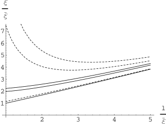
FIG. 1.: $\xi_{s}^{\min}(t,l)$ of Eq.20 (solid lines) plotted against l, in units of $\overline{\xi}$, for t=0, 3$\overline{\xi}$ and 4$\overline{\xi}$. $\xi_{s}^{\max}(t,l)$ of Eq.24 (dashed lines) plotted against l for t=0, 3$\overline{\xi}$ and 4$\overline{\xi}$. In each case the higher lines correspond to higher values of time

REFERENCES

- [1] T.W.B. Kibble, J. Phys. A9, 1387 (1976).
- [2] T.W.B. Kibble, in Common Trends in Particle and Condensed Matter Physics, Physics Reports 67, 183 (1980).
- [3] W.H. Zurek, Nature 317, 505 (1985), Acta Physica Polonica B24, 1301 (1993). See also W.H. Zurek, Physics Reports 276, Number 4, November 1996
-
[4]
W.H. Zurek, Nature 382, 297 (1996),
P. Laguna and W.H. Zurek, Phys. Rev. Lett. 78, 2519 (1997). A. Yates and W.H. Zurek, hep-ph/9801223. - [5] G. Karra and R. J. Rivers, Phys. Rev. Lett. 81, 3707 (1998).
- [6] D. Ibaceta and E. Calzetta, hep-ph/9810301 (1998).
- [7] P.V.E McClintoch et al., Phys. Rev. Letters 81, 3703 (1988).
- [8] B.I. Halperin, published in Physics of Defects, proceedings of Les Houches, Session XXXV 1980 NATO ASI, editors Balian, Kléman and Poirier (North-Holland Press, 1981) p.816.
- [9] F. Liu and G.F. Mazenko, Phys. Rev. B46, 5963 (1992).