[
Field dependence of the vortex structure in -wave and -wave superconductors
Abstract
We study the vortex structure and its field dependence within the framework of the quasi-classical Eilenberger theory to find the difference between the - and -wave pairings. We clarify the effect of the -wave nature and the vortex lattice effect on the vortex structure of the pair potential, the internal field and the local density of states. The -wave pairing introduces a fourfold-symmetric structure around each vortex core. With increasing field, their contribution becomes significant to the whole structure of the vortex lattice state, depending on the vortex lattice’s configuration. It is reflected in the form factor of the internal field, which may be detected by small angle neutron scattering, or the resonance line shape of SR and NMR experiments. We also study the induced - and -wave components around the vortex in -wave superconductors.
pacs:
PACS numbers: 74.60.Ec, 74.60.Ge, 74.72.-h, 76.75.+i.]
I Introduction
Much attention has been paid to the vortex structure in high- superconductors. Many researchers try to detect the -wave nature of the superconductivity in the vortex structure of the mixed state. It is necessary to clarify how the difference between the -wave and conventional -wave pairings appears in the mixed state. The point is how the vortex structure is affected by the anisotropy of the energy gap in the -wave pairing, particularly by its nodal structure. It is known that the difference appears in the field () dependence of the zero-energy density of states (DOS) . Volovik [1] theoretically suggested that the dependence is given by in the -wave pairing and in the -wave pairing. The difference between the two pairings was indeed confirmed by the self-consistent calculation of the quasi-classical Eilenberger theory for the vortex lattice case, but the field dependence of deviates from the exact - or -linear behavior. [2] In this paper, by using the quasi-classical method, we discuss other -wave natures appearing in the vortex structure, such as the pair potential, the internal magnetic field and the local density of states (LDOS).
Low energy excitations, which dominantly govern the vortex structure, can be divided conceptually into three categories; (1) those from the continuum states associated with the nodal structure in the -wave pairing, (2) the core excitations from the bound states localized in a vortex core, and (3) the quasiparticle transfer between vortices, i.e., the vortex lattice effect. While many calculations for the -wave pairing such as Ref. [1] take into account only item (1), which is valid near the lower critical field , items (2) and (3) are also indispensable when considering the vortex state in general. In order to help establish the general features of the mixed state in both the - and -wave cases, one needs to calculate the vortex structure while taking into account all three factors on an equal footing. Through these efforts we may gain a more valid and vivid picture of the vortex for the whole region of ( is the upper critical field).
Detailed properties of the vortex structure, such as its field dependence, attract much attention even in the conventional -wave superconductors. Several important means to probe the vortex structure are now available experimentally in various superconductors, including high- superconductors. Specific heat experiments [3, 4, 5, 6] inform us of low energy excitations. Muon spin resonance (SR)[7, 8] and small angle neutron scattering (SANS) investigate the internal field distribution of the vortex structure. Scanning tunneling microscopy (STM)[9, 10, 11, 12] directly observes the LDOS. These data are often analyzed within conventional phenomenological theories such as the Ginzburg-Landau (GL) theory or the London theory. The GL theory is, strictly speaking, valid only near the transition temperature .[13] As for the London theory, which is applied near , the simple cutoff procedure for the core radius is too rough an approximation to estimate the exact contribution of the vortex core.[14, 15] In this sense it is necessary to develop a microscopic theory in order to correctly analyze valuable experimental data.
In this paper, we investigate various aspects of the vortex lattice structure based on the quasi-classical Eilenberger theory to clarify the difference in the vortex structure between the - and -wave pairings. The case of a magnetic field applied along the axis (or axis) is considered. We follow the method of Refs. [16] and [17], where the -wave pairing case was investigated. This method can be applied in most regions of the mixed state, i.e., and . We calculate both the pair potential and the vector potential self-consistently in the vortex lattice case. Then we discuss the spatial variation of the current and the internal field in detail. As for the single vortex case, the fourfold-symmetric vortex core structure of the -wave pairing was shown in Ref. [18] by the quasi-classical calculation. In the present paper, where we examine the vortex lattice case, we can see how this -wave nature and the vortex lattice effect affect each other. And we also study the field dependence of the vortex structure.
The rest of this paper is organized as follows. In Sec. II, we describe the method of the quasi-classical calculation. In Sec. III, we estimate the free energy for several configurations of the vortex lattice. There, the square lattice has lower free energy than the conventional triangular lattice at higher fields. In Sec. IV, we study the field dependence of the vortex structure (the pair potential, the current and the internal field) in the square lattice case. The form factor and the distribution function of the internal field are discussed in connection with the SANS and SR experiments. The vortex structure in the triangular lattice case is briefly discussed in Sec. V. We study the LDOS structure and the field dependence of the spatially averaged DOS in Sec. VI, and the structure of the induced order parameter of the other symmetry in Sec. VII. A summary and discussions are given in Sec. VIII.
II quasi-classical Eilenberger theory
Our calculations are performed following the method of Refs. [16] and [17]. We consider the case of the clean limit and the cylindrical Fermi surface. These are appropriate to high- superconductors and low-dimensional organic superconductors.
First, we obtain the pair potential and the vector potential self-consistently by solving the Eilenberger equation in the Matsubara frequency . We consider the quasi-classical Green functions , and , where is the center of mass coordinate of the Cooper pair. The direction of the relative momentum of the Cooper pair, , is denoted by an angle measured from the axis. The Eilenberger equation is given by [19]
| (1) | |||
| (2) | |||
| (3) | |||
| (4) | |||
| (5) |
where and is the Fermi velocity. The vector potential is written as in the symmetric gauge, where is a uniform field and is related to the internal field , where . As for the pair potential , we set for the -wave pairing and for the -wave pairing. Here, is the angle between the axis and the axis of the crystal coordinate. The self-consistent conditions for and are given as
| (6) |
| (7) |
where is the density of states at the Fermi surface, is the pairing interaction, with Rieman’s zeta function . is the GL parameter in the BCS theory, and is the uniform gap at . We set the energy cutoff . In the following calculations, energies and lengths are measured in units of and ( is the BCS coherence length), respectively.
By solving Eqs. (2)-(5) by the so-called explosion method [16, 17] under and of the vortex lattice case, we estimate the quasi-classical Green functions at discretized points in a unit cell of the vortex lattice. We obtain a new and from Eqs. (6) and (7), and use them at the next step in calculating of Eqs. (2)-(5). This iteration procedure is repeated until a sufficiently self-consistent solution is obtained. We use the material parameters appropriate to YBCO, i.e., =16Å and =100. There, =66.7 Tesla in the -wave pairing and 93.2 Tesla in the -wave pairing for . [20] To study the field dependence, the calculations are done for various fields at a fixed temperature . The spatial variation of the internal field and the current is calculated from .
III vortex lattice configuration
We have to fix the shape and the orientation of the vortex lattice before calculation. The shape of the vortex lattice is characterized by the unit vectors and where and where the axis is set in the direction. Since we consider the case , we can write , where is the angle between and .
In this paper, we study the contributions of the -wave effect and the vortex lattice effect on the vortex structure. As the -wave nature reflects the node direction of the energy gap, its directional dependence is determined by the angle from the crystal coordinate. To investigate the -wave nature, we compare the vortex structure along the axis and axis directions (we denote these directions as “the directions” in the following) and that along the directions from the axis (we denote these as “the directions”). On the other hand, to study the vortex lattice effect, we compare the vortex structure along the nearest neighbor (NN) vortex direction and that along the next nearest neighbor (NNN) vortex direction. We denote the former direction as the “NN direction”, and the latter direction as the “NNN direction”. The orientation of the vortex lattice, i.e., the relative angle between the “ directions” and the “NN direction” is important in considering the vortex lattice structure in the -wave pairing. The orientation is characterized by .
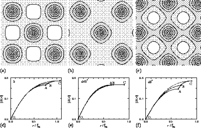
In an isotropic -wave superconductor, the shape of the vortex lattice is a triangular lattice. However, in a -wave superconductor, the shape may deviate from a triangular lattice. The deviation comes from the fourfold-symmetric vortex structure around the vortex core, which reflects the -wave symmetry of the pair potential in the space (i.e., ). To determine the vortex lattice configuration of the equilibrium state, we compare of Eq. (11) for the various vortex lattice configurations, and find the state having minimum . As our quasi-classical calculation needs a lot of time to compute, we cannot check all possible configurations of shape and orientation. So, we only compare the square lattice case () and the triangular lattice case () in the -wave pairing. There, we consider the two orientation cases and . For (), one of the NN vortices is located in the () direction. The field dependence of is shown in Fig. 1. There, we present the difference , where is for the case of the square lattice with . The square lattice with has the smallest at a higher field . At a lower field, the triangular lattice case has the smallest . So, the vortex lattice configuration changes from the triangular lattice to the square lattice with as the field increases. We note that there may be a stable oblique lattice between the triangular lattice and the square lattice. An estimate including the oblique lattice by the quasi-classical theory belongs to a future work. As the square lattice with has a higher , it is an unstable state. As for the orientation of the triangular lattice, the case has a smaller than the case , but the difference is very small.
Some theoretical calculations considered the vortex lattice configuration near , [21, 22, 23] or based on the London theory.[24, 25, 26] These theories suggested that the vortex lattice configuration gradually changes from the triangular lattice to the square lattice with increasing field, and the oblique lattice is realized at a lower field before settling into the square lattice. The square lattice configuration with has lower free energy than that of the conventional triangular lattice over a wide region of higher fields and lower temperatures in the mixed state for the -wave pairing. This is consistent with the estimate of Fig. 1. An STM experiment on (YBCO) also suggested the square vortex lattice configuration in the -wave pairing. [11]
IV vortex structure in the square lattice case
As noted in the previous section, the stable configuration of the vortex lattice at higher field is the square lattice with . We fix the shape of the vortex lattice as the square lattice in order to study the field dependence of the vortex structure. To clarify the roles of the -wave effect and the vortex lattice effect, we present the results of the unstable orientation case in addition to the stable orientation case in the -wave pairing. We denote the former as “the case”, and the latter as “the case”. The -wave pairing case is also calculated for the square lattice to clarify the effect of low lying excitations associated with the gap anisotropy. The comparison among these cases (-wave case, case and case) helps us to understand the contributions of the -wave nature and the vortex lattice effect.
A Amplitude of the pair potential
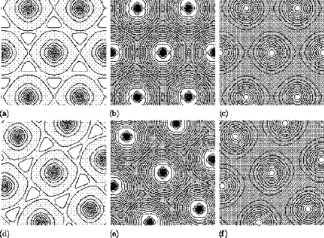
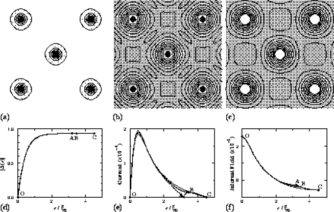
In Fig. 2, we show the spatial variation of the vortex structure at low field for the case. We show their contour lines and their profile. The profile is presented along the lines OA, OB, OC and AC shown in Fig. 3. The line OA (OC) is the radius in the NN (NNN) direction, and the line AC is along the boundary of the Wigner-Seitz cell of the vortex lattice.
The amplitude is presented in Figs. 2 (a) and (d). At low field, the vortex core region occupies a small part of a unit cell of the vortex lattice. There, approaches a constant value ( for ) at a few away from the vortex center, as presented in Fig. 2 (d). The -wave nature appears in the shape of the contour lines of . In the -wave pairing, the contour lines are circular around each vortex center at low field. In the -wave pairing, as shown in Fig. 2 (a), the contour lines become a fourfold-symmetric shape, especially for . There is suppressed around the vortex core in the directions compared with the directions. This structure is consistent with that obtained by the single vortex calculation. [18]
Figure 4 shows at a higher field for three cases. At high field, the vortex core region occupies a large part of a unit cell. So, does not reduce to a uniform value even in the boundary region, as shown in Figs. 4 (d)-(f). The influence of the vortex lattice effect on can be seen in Figs. 4 (a) and (d) for the -wave pairing case. While the vortex core has a circular symmetric structure in the inner region of the core (), shows directional dependence in the outer region, reflecting the NN vortices. There, is suppressed in the NN directions (line OA) compared with the NNN directions (line OC). In the -wave pairing, the contribution of the fourfold-symmetric core structure appears in addition to the vortex lattice effect, depending on the vortex lattice’s configuration, and especially on its orientation. We demonstrate this by showing two orientation cases [Figs. 4 (b) and (e)] and [Figs. 4 (c) and (f)]. In both cases, the inner region of the vortex core shows a fourfold-symmetric structure, seen also in the low field case shown in Fig. 2 (a). However, the difference between the two orientation cases appears in the outer region of the vortex core. Due to the -wave nature, is suppressed in the directions. Because of the vortex lattice effect, is suppressed in the NN directions. When these two directions disagree as in Fig. 4 (b), these two suppressions cancel each other. The difference between in the NN direction (line OA) and in the NNN direction (line OC) is smeared. Along the boundary line AC, is almost constant. On the other hand, when the direction and the NN direction agree as in Fig. 4 (c), the suppressions due to the vortex lattice effect and the -wave effect enhance each other. is largely suppressed in the directions (i.e., the line OA in the NN direction) compared to in the direction (i.e., the line OC in the NNN direction). The result shown in Fig. 1, which shows that the case is stable at higher field and the case is unstable, may be related to the difference in the vortex structure shown in Figs. 4 (b) and (c).
Next, we study the field dependence of . We define () as the maximum of along the line OA (OC) in the NN (NNN) direction. The field dependence of and is presented in Fig. 5 for the -wave (a) and the -wave (b) pairings. They decrease to 0 as is approached. The difference between and , which reflects the vortex lattice effect, appears when . The difference is small for the case, but large for the case, as discussed above.
The field dependence of the core radius is shown in Fig. 6. The radius is defined from the initial slope of the pair potential by setting as at the vortex center. As increases, the radius decreases similarly for both the -wave and the cases. In the unstable case, the decrease of is saturated at a higher field compared to the other cases.
B Internal current distribution
The spatial variation of the current at low field is shown in Figs. 2 (b) and (e) for the case. There, has four peaks around each vortex core in the directions at . The four peaks are -wave nature, and are consistent with the single vortex calculation. [18] In the -wave pairing at low field, distributes circularly around each vortex without four peaks. Outside the vortex core region (), there is no clear difference between the - and -wave pairings in the current distribution.
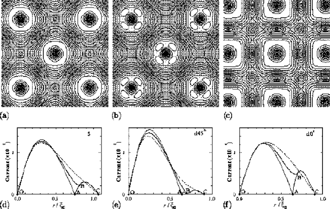
Figure 7 shows at high field , which corresponds to the case of Fig. 4. In the -wave pairing case of Fig. 7 (a), there are four peaks around each vortex core in the NN vortex directions. These peaks are due to the vortex lattice effect and enhance the four peaks of the -wave nature in the directions for the case [Fig. 7 (b)], but smear them for the case [Fig. 7 (c)].
We can also define the core radius by the maximum current. The core radius is defined as the radius where is at a maximum in the NN vortex direction. The field dependence of is presented in Fig. 6 (b). The radius decreases similarly to as shown in Fig. 6 (a). From both definitions of and (i.e., the initial slope of and the maximum current), we obtain a similar dependence on . The shrinkage of the core radius was also reported in STM and SR experiments. [10, 7] There, the results of the field dependence were analyzed in the dirty limit theory by the Wigner-Seitz method (i.e., a circular unit cell is used instead of the periodic boundary condition of the vortex lattice). In our study, we obtain the field dependence in the clean limit, where we treat the periodic boundary condition exactly.
The radius is also presented for the triangular vortex lattice of the -wave pairing[Fig. 6]. The field dependence is almost the same as in the square lattice case of the -wave pairing. We confirm that the core radius of the -wave pairing shows a similar decrease to the triangular vortex lattice case[Fig. 6]. When we calculate the radius for a smaller () in the -wave pairing to study the case of , a similar decrease is obtained. So, the decrease of the core radius occurs over a wide range of .
C Internal field distribution
Reflecting the four peaks of in the directions, the internal field distribution has a fourfold-symmetric structure around each vortex core, as presented by the single vortex calculation.[18] extends toward the directions in which the screening current is weak. However, this fourfold-symmetric structure is restricted to the vortex core region, since the -wave nature is compensated by outside the core. Outside the core region, immediately reduces to a circular structure. This compensation is seen in the single vortex case,[18, 27] but it also appears in the vortex lattice case at low field. In Fig. 2 (c) and (f), we show the spatial variation of at low field for the case. In the -wave pairing, the contour lines of in the vortex core region are distorted from the circle of the -wave pairing case into a fourfold symmetry. The distortion can be seen within the small core region as shown in Fig. 2 (c). Outside the core region, recovers the circular contour lines seen in the -wave case. So the -wave nature scarcely affects the internal field distribution at low field. In the -wave pairing case, has the same structure as that shown in Fig. 2 (c) except for the small region of the vortex core.
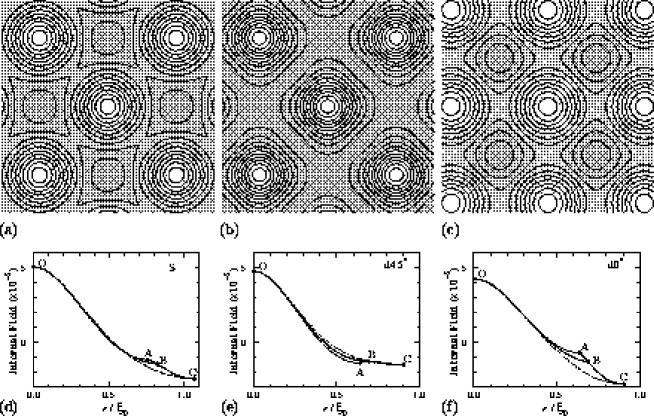
Figure 8 shows at high field =0.54, which corresponds to the case shown in Fig. 7. In the -wave pairing, is lowest at the boundary of the NNN direction (i.e., the point C in Fig. 3). There is a saddle point in at the boundary of each NN direction (i.e., the point A in Fig. 3). The fourfold symmetry around the vortex core due to the -wave nature is seen in Figs. 8 (b) and (c), where is enhanced in the directions, and suppressed in the directions. In the case in Fig. 8 (b), the -wave nature enhances at the minimum point in the NNN direction, and suppresses it at the saddle point in the NN direction. So, variation of along the boundary line AC is small. On the other hand, for the case in Fig. 8 (c), is enhanced at the saddle point and suppressed at the minimum point due to the -wave nature. So, the difference between the field at the saddle point A and the field at the minimum point C is large. Since the distribution is observed in SANS and SR experiments, we discuss the related quantities in detail.
First, we investigate the form factor of . It is measured by the SANS experiment. The form factor ( and are integers) is the Fourier component of defined as
| (16) |
where the reciprocal lattice vector , where , and with and . The field dependence of the dominant form factor is plotted in Fig. 9 for the - and -wave pairings. The two pairing cases show a similar dependence on the applied field. So, it is difficult to detect the -wave nature in . However, we can detect it in the higher order components such as and . The field dependence of , , and is plotted in Fig. 10. The effect of the -wave nature appears depending on the orientation of the vortex lattice. As shown in Fig. 10 (a), with increasing field, of the -wave pairing decreases and becomes negative. In the stable case, remains positive. However, in the unstable case, decreases more rapidly than that of the -wave pairing. As shown in Fig. 10 (b), remains almost constant at high field in the -wave pairing. In the case, increases as is approached. But, in the case, it decreases. For and for , the -wave effect shifts the form factors in the opposite direction. The -wave nature also appears in [Fig. 10 (c)] and [Fig. 10 (d)]. We expect that these -wave natures can be detected by the SANS experiment. The form factors are also presented for the triangular vortex lattice of the -wave pairing in Figs. 9 and 10. Their field dependence is qualitatively the same as in the square lattice case of the -wave pairing.
Next, we investigate the magnetic field distribution function defined as
| (17) |
It corresponds to the resonance line shape in SR or NMR experiments. In Fig. 11, we plot for =0.021(a), 0.15(b) and 0.54(c) in the -wave pairing case and in the two orientation cases of the -wave pairing. We denote the maximum (minimum) of as (). Reflecting the saddle point in , has a logarithmic singularity at . In the low field case shown in Fig. 11 (a), is almost the same shape for both the - and -wave pairings. For comparison, we also present the line shape of the triangular lattice case in Fig. 11 (a), which also does not show any difference between the - and -wave pairings. As shown in Fig. 2 (c), the -wave nature scarcely appears in at a low field. With increasing field, the -wave nature gradually appears in as shown in Figs. 11 (b) and (c). For the stable case, increases and decreases compared with the -wave pairing case, as shown in Fig. 8 (b). For the unstable case, decreases and increases. These changes of and can be seen in the resonance line shape in Figs. 11 (b) and (c). We note that the line shape of the case in Fig. 11 (c) resembles that of the triangular lattice (see Fig. 11 (a)). So, in the -wave pairing, it is risky to determine the vortex lattice shape by the conventional method based on the distance between and , i.e., . The field dependence of , and is presented in Fig. 12. There, shows a similar dependence for both the - and -wave pairings. We also calculate the field dependence of in the triangular vortex lattice for the -wave and -wave pairings. Their dependence is almost the same as that of the square lattice case. So, is not much affected by the vortex lattice configuration and the pairing symmetry. The -wave nature affects and . For the stable case, approaches with increasing field, and for . We hope that this characteristic of the resonance line shape will be examined by the SR or NMR experiments.
To help in analyzing the shape of the distribution function , we plot the field dependence of the variance and of the skewness parameter in Fig. 13. These quantities are analyzed by the SR experiment.[15, 28, 29, 30] As for the variance, both the - and -wave pairings show a similar dependence on . But, the difference between the - and -wave pairings clearly appears in the skewness parameter.
V Vortex structure in the triangular lattice case
To study the vortex structure at low field and the effect of the vortex lattice shape, we also consider the triangular vortex lattice case. In Fig. 14, we show the vortex structure at for the -wave pairing. The contour lines of , and are presented for the two orientation cases and . The contour lines of show a fourfold-symmetric shape, has four peaks in the directions, and extends in the direction around each vortex core. These features show the -wave nature presented in the previous section. At a low field such as , the fourfold-symmetric structure of the -wave nature is restricted to the small region of the vortex core as in the case shown in Fig. 2. These core structures are not affected by the shape and the orientation of the vortex lattice at low field. But, with increasing field, the fourfold-symmetric core structure gradually feels the effect of the hexagonal Wigner-Seitz cell of the vortex lattice. By the effect of the fourfold-symmetric structure around the core region, the six NN directions of the triangular lattice are not equivalent in the -wave pairing. In Fig. 14 (a) for , the suppression of in the NN directions due to the vortex lattice effect is enhanced in the axis direction by the -wave nature. So, the structure of the two NN directions along the axis is not equivalent to that of the other four NN directions. The suppression due to the -wave nature in the axis direction is weakened by the vortex lattice effect because it is in the NNN direction. The vortex structure now shows twofold symmetry, which becomes more prominent at higher field. In Fig. 14 (d) for , the suppression in the NN direction is weakened in the direction, compared with the other four NN directions.
The structure of these two NN directions can also be seen in the current [Figs. 14 (b) and (e)] and the internal field [Figs. 14 (c) and (f)]. In Fig. 14 (c) for , at the two saddle points in the axis NN direction is larger than that of the saddle points in the other four NN directions. In Fig. 14 (f) for , at the two saddle points in the direction becomes small compared to the other four NN directions. The resonance line shape in the triangular lattice case is presented in Fig. 15, where the line shape around the peak is focused. Reflecting the two saddle points of in Figs. 14 (c) and (f), the line shape of has two logarithmic peaks in the -wave pairing. The two peak structure was suggested for the oblique lattice state between the square lattice and triangular lattice, based on the GL theory or the London theory.[14, 21, 31] But, it occurs even in the triangular lattice for the -wave pairing by the influence of the fourfold-symmetric vortex core structure.
Relaxing the difference between these two NN directions, the shape of the vortex lattice may deviate from the triangular lattice. For in Fig. 14 (a), the intervortex distance in the axis NN directions may increase compared with the other NN directions. For in Fig. 14 (d), the intervortex distance in the directions may decrease compared with the other NN directions. This deformation may relax the difference between the two NN directions. This is the origin of the distortion from the conventional triangular lattice. The oblique lattice is realized in the intermediate field region between the square lattice and the triangular lattice. In the oblique lattice, the double-peaked structure of shown in Fig. 15 may be smeared, since the difference of the two saddle points is weakened by the distortion from the triangular lattice.
VI Density of states
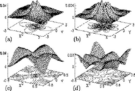
The LDOS is calculated by Eq. (8) in the square vortex lattice case for the -wave and the cases. Typically, we choose . First, we discuss the LDOS for the -wave pairing. In the calculation for a single vortex, the LDOS for low energy excitations is mainly distributed in a circle around the vortex center.[32, 33] The radius of the circle increases if is raised. The LDOS of the vortex lattice case is presented in Fig. 16 for the -wave pairing at . The area presented is the Wigner-Seitz cell of the square vortex lattice, i.e., within the dotted line shown in Fig. 3. The LDOS for low energy excitations is distributed in a circle as in the single vortex case. Further, by the vortex lattice effect (i.e., the quasiparticle transfer between vortices), is suppressed on the line connecting two NN vortex centers, as shown in Fig. 16 (a). A small suppression also occurs along the line between two NNN vortex centers. For a finite below , the suppression occurs in the NN directions along the tangent lines of the circle of the dominant LDOS distribution, as shown in Fig. 16 (b) and (c). The suppression is scarcely seen at low field . There, the LDOS distribution shows an almost circular symmetry around each vortex. At high field, however, the suppression becomes significant and the LDOS distribution deviates from the circular symmetry and shows fourfold-(sixfold-)symmetric structure in the square (triangular) lattice case, reflecting the vortex lattice effect.[17] At high field, the LDOS has a finite distribution all over the unit cell in addition to the ridge structure, while at low field it is distributed in a restricted region along the circular ridge.
Next, we discuss the -wave pairing case. The single vortex calculation shows that the LDOS for low energy excitations around a vortex has prominent tails extending in the directions [see Fig. 8 (d) of Ref. [18]], reflecting the node structure of the energy gap in the -wave pairing. Since the low energy quasiparticle distribution around a vortex extends toward infinite points in the directions, this low energy state is not a bound state in the exact meaning.[34] The LDOS of the vortex lattice case is presented in Fig. 17 at for the case. In this configuration, the directions are the NN vortex directions, which are on the axis and axis in the figure. In in Fig. 17 (a), the tail structure in the directions in the single vortex case is modified due to the vortex lattice effect. Each tail of the zero energy LDOS in the directions splits into two ridges because of the suppression by the vortex lattice effect in the NN vortex directions. So, the tails extend in rather different directions from the directions. In the -wave pairing, the suppression of the vortex lattice effect occurs from a low field such as . It means that the quasiparticle transfer between vortices is large due to the tail structure of the LDOS in the -wave pairing, compared with the -wave pairing case. With increasing field, the vortex lattice effect increases and the splitting of the tail structure in the directions becomes pronounced.
For a finite below the energy gap , shows a “#”-shape ridge structure in the -wave pairing, as shown in Fig. 17 (b) and (c). This is consistent with the calculation for the single vortex case.[18, 33] The ridge structure is not much affected by the vortex lattice effect except when . The reason is as follows. The quasiparticle flow is along the ridges on the four open trajectories.[18] When the flow direction of the quasiparticles on the trajectories approaches the directions, it leaves the vortex center. There, the quasiparticles with a finite become a scattering state, since is satisfied. When the quasiparticle flow is toward the NN vortex directions, the vortex lattice effect occurs. However, since the NN directions are now the directions, the quasiparticles flowing toward the NN vortex directions on the trajectories are in a scattering state. A scattering state is widely distributed and does not contribute to the ridge structure.
As a result, the local spectrum is given as follows in the vortex lattice state. There are some peaks below the energy gap as in the single vortex case, reflecting the trajectory structure.[18] Extra small peaks may also appear by the trajectories extending from neighboring vortices. And the low energy state for is suppressed due to the vortex lattice effect on the line connecting two NN (or NNN) vortex centers.
We have considered the case of the square lattice with . From that information, we can estimate the spatial variation of in the other vortex lattice configuration. First, we consider the contribution on from the vortex core and the four tails extending in the directions from each vortex center. The suppression along the line connecting NN vortices is also taken into account. There is also a small suppression in the NNN vortex directions. The suppression is larger at higher field. Then, we obtain the structure in the other vortex lattice configuration.
The relation is sometimes considered for the -wave pairing. The relation is based on the single vortex calculation,[1] which yields a structure with four tails extending in the directions. These result from the node structure of the energy gap. However, since the vortex lattice effect smears the tail structure, the relation may be affected. We examined it in Ref. [2] and obtained . The exponent becomes smaller than . The relation is sometimes considered for the -wave pairing. In this case, is proportional to the vortex density since the low energy excitation consists of a bound state around each vortex core. We also examined this case in Ref. [2] and obtained . The deviation from the -linear relation results from the field dependence of the vortex core radius which we presented in Fig. 6.
The spatially averaged DOS in Eq. (9) is presented in Fig. 18 for the -wave (a) and -wave (b) pairings. We note that the energy gap in the -wave case is in Fig. 18 (b). The energy gap structure at zero field is gradually buried by the low energy excitation of the vortex as the field increases. While the local spectrum has several peaks depending on the pairing symmetry and the position,[18] there is no peak in below the energy gap. The peak structure is smeared when the spatial average is taken.
VII Induced order parameter of other symmetry
So far, we have considered the case where we can neglect the induced order parameter of other symmetry, i.e., the pure -wave case. When there is -wave (-wave) interaction in addition to the dominant -wave pairing interaction, the -wave (-wave) component of the pair potential is induced at the place where the dominant -wave pair potential spatially varies, such as a vortex or an interface. The induced -wave component was mainly studied by the two-component GL theory, where the coupling of the -wave and the -wave components in the gradient term plays an important role.[31, 35] The induced -wave component can be discussed by extending the two component GL theory by including the higher order gradient coupling.[36] The quasi-classical calculation for the induced -wave and -wave components was performed for the single vortex case.[36] The induced component around the vortex was also reported in a study of the Bogoliubov-de Gennes theory for several models.[34, 37, 38, 39] There, the amplitude of the induced component depends on the interaction parameter and the carrier density.
In this section, we study the spatial structure of the induced - and -wave components in the vortex lattice of -wave superconductors, based on the quasi-classical theory. These induced components can be calculated using Eq. (6), by setting
| (19) | |||||
| (21) | |||||
where , and . Note that the induced components and are, respectively, proportional to and . Here, we consider the case . In this case, the contributions of and are small and can be neglected compared to the dominant contribution in the calculation of Eqs. (2)-(5).
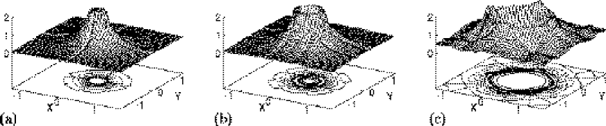
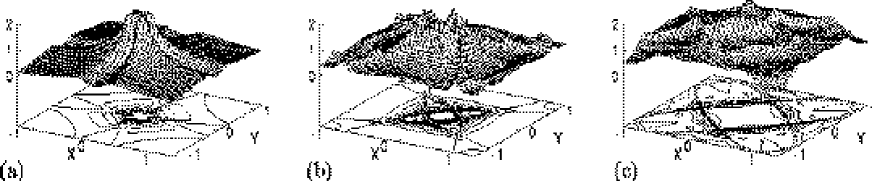
Figure 19 shows the spatial variation of the amplitudes and in the case at low field and high field . The presented area is the Wigner-Seitz cell of the square vortex lattice, i.e., within the dotted line in Fig. 3. At low field, the contour line of is a four-lobed shape, as shown in Fig. 19 (a). There, has four peaks around the vortex core in the directions (which correspond to the axis and axis in this figure). The contour line of is eight-lobed shape shape, as shown in Fig. 19 (b). There are eight peaks of around the vortex core in the and directions. These structures of and at low field are consistent with those found in a single vortex.[36] With increasing field, since the size of the unit cell decreases, the structures of and gradually change to those shown in Figs. 19 (c) and (d), respectively. These structures have extra zero points on the boundary in addition to the vortex center.
To understand the structures of and , we present the structure of the phase schematically for low and high field in Fig. 20. There, the position of the singularity and its winding number are presented for the relative phase to the dominant , i.e., and . Since has the singularity of the winding number at the vortex center, the winding number of itself is at the vortex center [the case shown in Fig. 20 (a) and (c)]. And that of is at low field [Fig. 20 (b)] and at high field [Fig. 20 (d)]. The singularity corresponds to the zero point of the amplitudes and in Fig. 19. Around the singularity of the winding number , the amplitude increases as .
At low field, as shown in Fig. 20 (a), the relative phase of the -wave component has a singularity at the vortex center and four singularities in the directions. This is consistent with the single vortex case.[17] Since the winding number of the relative phase should total zero for each unit cell to satisfy the periodic boundary condition, there is a singularity at each corner of the Wigner-Seitz cell. With increasing field, the singularity approaches the boundary and the four singularities combine with the singularities at the corners producing singularities, as shown in Fig. 20 (c). In the triangular vortex lattice case, each () singularity at the corner of the boundary splits into two () singularities which are located at the corner of the hexagonal Wigner-Seitz cell.
On the other hand, has a singularity at the vortex center and eight singularities around the vortex core at low field. This is consistent with the single vortex case.[36] Further, to satisfy the periodic boundary condition, there are eight singularities on the boundary, as shown in Fig. 20 (b). As the field increases, the singularities approach the singularities on the boundary, becoming singularities on the boundary, as shown in Fig. 20 (d). The singularity at the vortex center splits into four singularities around the vortex core.
We also consider the case, where the direction is along the and axes. The four-peaked structure of at low field rotates from its position in the case [Fig. 19 (a)]. The low field structure is fixed to the crystal coordinate. However, as the field increases, the structure of reduces to that shown in Fig. 19 (c). The high field structure is independent of the crystal coordinate and is fixed to the shape of the vortex lattice. On the other hand, the structure of is the same as in the case regardless of the field.
Even in an -wave superconductor, if the extra -wave (-wave) component exists in the interaction, () is induced around the vortex. We also calculate its structure in the vortex configuration shown in Fig. 4 (a). The induced () has the same structure as in the () case.
The induced component may be discussed qualitatively by the two component GL theory.[21, 31, 35, 36] There, the vortex structure was studied in the single vortex case near and in the vortex lattice state near . The results agree with ours. Near , the vortex structure is described by the magnetic Bloch state function , where represents the -th Landau level.[21] As for the dominant -wave pair potential, in the leading order. For the induced -wave component, since it is induced by the gradient coupling in the GL equation. For the induced -wave component, since it is induced by the gradient coupling in the extended GL equation.[36] In fact, at high field, and as obtained by our calculation have the same structure as and , respectively.
VIII Summary and Discussions
We have studied the vortex structure and its field dependence in the -wave and -wave superconductors by the self-consistent calculation of the quasi-classical Eilenberger theory for the vortex lattice case. At a higher field, the square vortex lattice configuration with (i.e., the NN vortex is located in a direction from the axis) has lower free energy than the conventional triangular lattice for the -wave pairing. Then, we investigated the field dependence of the vortex structure in the square lattice configuration. Due to the -wave nature, the contour lines of the amplitude and the internal field show a fourfold-symmetric shape around the vortex core. The fourfold-symmetric structure is prominent in the vortex core region. At low field, the -wave nature scarcely affects the structure of the outer region of the core. With increasing field, the core region occupies a larger area of the unit cell in the vortex lattice. Then, the -wave nature gradually affects the whole structure of the vortex lattice. It affects the form factor of and the magnetic field distribution function. The former is detected by the SANS experiment, and the latter corresponds to the resonance line shape in the SR and NMR experiments. At higher field, we also have to consider the vortex lattice effect on the vortex structure. The orientation of the vortex lattice (i.e., the relative angle between the axis and the NN vortex direction) is important for the vortex structure.
The vortex core radius decreases similarly for both the -wave and the -wave pairing with increasing field. In the triangular vortex lattice case, the six NN directions are not equivalent in the vortex structure for the -wave pairing. This may be the origin of the distortion from the triangular lattice. We showed the influence of the -wave nature and the vortex lattice effect on the LDOS, and discussed the field dependence of the spatially averaged DOS. The spatial structure of the induced -wave and -wave order parameter in the -wave superconductor was also presented. We note that the effect of the induced order parameter was not included in our discussion of the -wave nature in Secs. III-VI. The -wave nature appears even when the induced order parameter of the other symmetry is absent.
The -wave nature of the vortex structure , and was also studied in the GL theory or the London theory by including nonlocal correction terms. We note that the GL theory only applies by the exact derivation near .[13] For other cases, we have to include nonlocal correction terms. We usually consider only the fourth order derivative terms as non-local terms, which contribute to the vortex structure in the correction of the order . But, at lower temperature, we have to include higher order derivative terms. Their contribution is a higher order of . Further, as we increase the amplitude of the order parameter bellow , we also have to consider higher order nonlinear terms of the order parameter than the usual term. It is difficult to consider all contributions of these higher order terms by modifying the GL theory. The quasi-classical Eilenberger theory automatically includes all contributions of the higher order terms. Nevertheless, the -wave nature and the vortex lattice effect obtained by the quasi-classical calculation can be reproduced qualitatively by the GL theory with the correction of the fourth order derivative terms.[21, 27] We note that the -wave nature in the resonance line shape is also reproduced.[21] This means that the extended GL theory is still useful as a phenomenological theory for the qualitative study of the -wave nature in the vortex structure. The validity of the study with the nonlocal correction term (i.e., fourth order derivative term) in the GL theory or London theory[24, 25, 26] can be confirmed by a comparison with the result obtained in a microscopic theory such as the quasi-classical theory. But, for a quantitative study, we have to use a microscopic theory.
In the London theory, the amplitude of the pair potential is treated as a constant outside the small region of the vortex core. However, this is only justifiable if the field is low enough. In our calculation where , shows a spatial variation at every region of a unit cell for . We have to carefully use an approximation of the constant amplitude over a wide range of the applied field.
We expect that the -wave nature presented in this paper will be observed in experiments on the -wave superconductors such as the high superconductors and the organic superconductors.[40] We recommend that the vortex structure be investigated into the higher field range, where the -wave nature is eminent. At lower fields, we also consider the effect of the gradual transformation from the triangular to the square vortex lattice. Borocarbide superconductors such as are also good candidates for observing the -wave nature.[5] These materials are considered to be -wave superconductors or -wave superconductors with a highly anisotropic Fermi surface with fourfold symmetry. Even for the latter -wave case, we obtain a similar vortex structure to the -wave pairing case by the -dependence of instead of the -dependence of .[41] There, the -direction of large plays the same role as the small direction. In experiments on , the fourfold-symmetric behavior of is reported when the field direction is rotated within the plane.[42] From the anisotropy, the magnitude of the -wave-like behavior is estimated as =0.43, where means the average on the Fermi surface. This magnitude is comparable to 0.25 of the -wave pairing case ( and an isotropic 2D Fermi surface). So, the large -wave-like anisotropy effect is expected in the vortex structure. The gradual transition from the triangular to the square vortex lattice is also observed with increasing field.[23, 43] As SR and SANS experiments have begun on these materials, we expect that the -wave-like nature will be detected there.
For the other symmetry of the anisotropic superconductors such as heavy fermion superconductors or , if the -dependence of their pair potential or the Fermi surface structure has a large anisotropy in the directions perpendicular to the applied magnetic field, the anisotropy effect appears by the same origin as that discussed in this paper. It may give important information for determining the symmetry of the order parameter.
Acknowledgments
We would like to thank N. Hayashi and T. Sugiyama for their helpful comments. Some of the numerical calculations in this work were carried out at the Yukawa Institute Computer Facility, Kyoto University, and the Supercomputer Center of the Institute for Solid State Physics, University of Tokyo. One of the authors (M.I.) is supported financially by the Japan Society for the Promotion of Science.
REFERENCES
- [1] G. E. Volovik, JETP Lett. 58, 469 (1993).
- [2] M. Ichioka, A. Hasegawa, and K. Machida, Phys. Rev. B 59, 184 (1999).
- [3] K. A. Moler et al., Phys. Rev. Lett. 73, 2744 (1994).
- [4] R. A. Fisher et al., Physica C 252, 237 (1995).
- [5] M. Nohara et al., J. Phys. Soc. Jpn. 66, 1888 (1997).
- [6] M. Hedo et al., J. Phys. Soc. Jpn. 67, 33 (1998).
- [7] J. Sonier et al., Phys. Rev. Lett. 79, 1742 (1997).
- [8] J. Sonier et al., Phys. Rev. Lett. 79, 2875 (1997).
- [9] H. F. Hess et al., Phys. Rev. Lett. 62, 214 (1989); 64, 2711 (1990); Physica B 169, 422 (1991). H. F. Hess, Physica C 185-189, 259 (1991).
- [10] A. A. Golubov and U. Hartmann, Phys. Rev. Lett. 72, 3602 (1994).
- [11] I. Maggio-Aprile et al., Phys. Rev. Lett. 75, 2754 (1995); J. Low Temp. Phys. 105, 1129 (1996).
- [12] Ch. Renner et al., Phys. Rev. Lett. 80, 3606 (1998).
- [13] See, for example, N. R. Werthamer, in Superconductivity, ed. R. D. Parks (Marcel Dekker, New York, 1969).
- [14] E. H. Brandt, J. Low Temp. Phys. 73, 355 (1988).
- [15] A. Yaouanc, P. Dalmas de Réotier, and E. H. Brandt, Phys. Rev. B 55, 11107 (1997).
- [16] U. Klein, J. Low Temp. Phys. 69, 1 (1987); Phys. Rev. B 40, 6601 (1989). B. Pöttinger and U. Klein, Phys. Rev. Lett. 70, 2806 (1993).
- [17] M. Ichioka, N. Hayashi, and K. Machida, Phys. Rev. B 55, 6565 (1997).
- [18] M. Ichioka, N. Hayashi, N. Enomoto, and K. Machida, Phys. Rev. B 53, 15316 (1996).
- [19] G. Eilenberger, Z. Phys. 214, 195 (1968).
- [20] T. Sugiyama, private communication.
- [21] M. Ichioka, N. Enomoto, and K. Machida, J. Phys. Soc. Jpn. 66, 3928 (1997).
- [22] H. Won and K. Maki, Phys. Rev. B 53, 5927 (1996).
- [23] Y. De Wilde et al., Phys. Rev. Lett. 78, 4273 (1997). Their calculation of the GL theory can be applied to the -wave case.
- [24] V. G. Kogan, M. Bullock, B. Harmon, P. Miranović, Lj. Dobrosavljević-Grujić, P. L. Gammel, and D. J. Bishop, Phys. Rev. B 55, 8693 (1997).
- [25] M. Franz, I. Affleck, and M. H. S. Amin, Phys. Rev. Lett. 79, 1555 (1997). I. Affleck, M. Franz, and M. H. S. Amin, Phys. Rev. B 55, 704 (1997).
- [26] M. H. S. Amin, I. Affleck, and M. Franz, Phys. Rev. B 58, 5848 (1998).
- [27] N. Enomoto, M. Ichioka, and K. Machida, J. Phys. Soc. Jpn. 66, 204 (1997).
- [28] P. Dalmas de Réotier and A. Yaouanc, J. Phys. Condens Matter 9, 9113 (1997).
- [29] S. L. Lee et al., Phys. Rev. Lett. 71, 3862 (1993).
- [30] C. M. Aegerter et al., Phys. Rev. B 54, 15661 (1996).
- [31] A. J. Berlinsky, A. L. Fetter, M. Franz, C. Kallin, and P. I. Soininen, Phys. Rev. Lett. 65, 2200 (1995). M. Franz, C. Kallin, P. I. Soininen, A. J. Berlinsky, and A. L. Fetter, Phys. Rev. B 53, 5795 (1996).
- [32] S. Ullah, A. T. Dorsey, and L. J. Buchholtz, Phys. Rev. B 42, 9950 (1990).
- [33] N. Schopohl and K. Maki, Phys. Rev. B 52, 490 (1995).
- [34] M. Franz and Z. Tešanović, Phys. Rev. Lett. 80, 4763 (1998).
- [35] Y. Ren, J. H. Xu, and C. S. Ting, Phys. Rev. Lett. 74, 3680 (1995); Phys. Rev. B 53, 2240 (1996). J. H. Xu, Y. Ren, and C. S. Ting, Phys. Rev. B 52, 7663 (1995); 53, 2991 (1996).
- [36] M. Ichioka, N. Enomoto, N. Hayashi, and K. Machida, Phys. Rev. B 53, 2233 (1996).
- [37] P. I. Soininen, C. Kallin, and A. J. Berlinsky, Phys. Rev. Lett. 50, 13883 (1994).
- [38] Y. Wang and A. H. MacDonald, Phys. Rev. B 52, 3876 (1995).
- [39] A. Himeda, M. Ogata, Y. Tanaka, and S. Kashiwaya, J. Phys. Soc. Jpn. 66, 3367 (1997).
- [40] See, for example, Y. Nakazawa and K. Kanoda, Phys. Rev. B 55, 8670 (1997).
- [41] N. Hayashi, M. Ichioka, and K. Machida, Phys. Rev. B 56, 9052 (1997).
- [42] V. Metlushko et al., Phys. Rev. Lett. 79, 1738 (1997).
- [43] M. R. Eskildsen et al., Phys. Rev. Lett. 78, 1968 (1997).


![[Uncaptioned image]](/html/cond-mat/9901339/assets/x9.png)