Charge and Statistics of Quantum Hall Quasi-Particles

A numerical study of mean values and fluctuations

H. Kjønsberg^† and J. M. Leinaas

Department of Physics, University of Oslo

P.O. Box 1048 Blindern, N-0316 Oslo, Norway

ABSTRACT

We present Monte Carlo studies of charge expectation values and charge fluctuations for quasi-particles in the quantum Hall system. We have studied the Laughlin wave functions for quasi-hole and quasi-electron, and also Jain’s definition of the quasi-electron wave function. The considered systems consist of from 50 to 200 electrons, and the filling fraction is $1/3$. For all quasi-particles our calculations reproduce well the expected values of charge; $-1/3$ times the electron charge for the quasi-hole, and $1/3$ for the quasi-electron. Regarding fluctuations in the charge, our results for the quasi-hole and Jain quasi-electron are consistent with the expected value zero in the bulk of the system, but for the Laughlin quasi-electron we find small, but significant, deviations from zero throughout the whole electron droplet. We also present Berry phase calculations of charge and statistics parameter for the Jain quasi-electron, calculations which supplement earlier studies for the Laughlin quasi-particles. We find that the statistics parameter is more well behaved for the Jain quasi-electron than it is for the Laughlin quasi-electron.

^†Supported by The Norwegian Research Council.

1 Background, motivation and summary of main results

The perhaps most striking feature of the fractional quantum Hall effect is the existence of quasi-particles with fractional charge and statistics. There now exists direct experimental evidence for the existence of fractionally charged particles [1], but much of the evidence for fractional statistics in the quantum Hall system is still indirect and based on the theoretical description of the effect.

For the plateau states corresponding to filling fractions $\nu=1/m$, $m$ odd, the many-electron wave functions introduced by Laughlin [2] are generally accepted as giving an essentially correct representation of the true quantum states (under the idealized condition of a homogeneous background potential). Also the quasi-hole excitations are described by simple wave functions, and there are robust arguments for these to be essentially correct. The charge and statistics of the quasi-holes have been determined by Berry-phase calculations and agree with the claim that they are anyons [3]. The situation is less clear for the quasi-electrons. Different trial wave functions have been suggested, notably by Laughlin [2] and Jain [4], but the conclusions based on these are less convincing than those for the quasi-holes.

Although the indirect evidence for the charged excitations of the fractional quantum Hall effect to be anyons is rather convincing, a more direct verification would certainly be interesting. It is a challenge to establish experimental evidence for the (fractional) statistics of the charge carrying excitations in a similar way as their fractional charge has been found. However, also on the purely theoretical side it is of interest to examine further the anyon aspects of the quantum Hall effect.

In a previous paper [5] we examined the anyon representation of the Laughlin quasi-holes in some detail. In that paper also the quasi-electrons were discussed, although much more briefly. In particular it was pointed out that in order to reproduce expected values for charge and statistics parameters by Berry phase calculations, approximations had to be done which could not readily be justified. This motivated subsequent numerical studies of quasi-electrons, by Kjønsberg and Myrheim [6], for systems with up to 200 electrons. For the charge parameter bulk values were found which were close to the expected value. However, for the statistics parameter the rather surprising result was that no stable bulk value was found. The numerical studies were done by applying the quasi-electron wave functions introduced by Laughlin. These results were quite different from the corresponding numerical results obtained for quasi-holes.

The results obtained in Ref. [6] have motivated the present work, where we examine charge expectation values as well as charge fluctuations for quasi-holes and quasi-electrons. The fractional charge of the physical quasi-particles is expected to be a sharply defined quantum number, and it is of interest to check whether this is true for the suggested trial wave functions. There exist some general arguments which link fractional statistics to fractional charge [7], and although the precise conditions for this to be true are not clear, they suggest that the problems which are seen in Berry phase calculation of the statistics parameter may also show up in the charge calculations. We have in particular been interested in examining the possibility of long range fluctuations in the quasi-electron charge.

The calculations of expectation values and fluctuations of charge have been done by the Monte Carlo method for quasi-holes and quasi-electrons corresponding to the $m=3$ state. We have in particular compared results obtained with Laughlin’s [2] and Jain’s [4] definitions of the quasi-electron wave functions. The systems considered have electron numbers varying from 50 to 200. The main results of the calculations are the following:

For quasi-holes the expected bulk values of the charge and the charge fluctuations are well reproduced. The expectation value of the charge is $-1/3$ (times the electron charge) and the charge fluctuation is zero. Numerically small statistical fluctuations are present, but no significant deviations from these values. For Laughlin’s quasi-electron the numerical results for the charge expectation values are consistent with the expected value $1/3$. However, for the charge fluctuations we find small, but statistically significant deviations from the value zero in the bulk. This is the case even for an electron number of 200. For Jain’s definition of the quasi-electron wave function we again reproduce expected results, $1/3$ for the charge and vanishing fluctuations. Differences between these values and the numerical results are within small statistical errors.

These results indicate that the problems earlier found in Berry phase calculations of the statistics parameter [6] may be an artifact of Laughlin’s special definition and not a signal of long range effects for a generic quasi-electron state. To check this more directly we have also examined the charge and statistics parameters found from Berry phase calculations of the Jain quasi-electron state. We find for this wave function a stable bulk value of the statistics parameter consistent with the value $-1/3$.

Throughout the paper, we are using dimensionless complex coordinates $z=\frac{1}{{\sqrt{2}}\ell_{B}}(x+iy)$, with $\ell_{B}=1/\sqrt{eB}$, and we set $\hbar,c=1$, $B$ being the magnetic field.

2 Quasi-particle charge and charge fluctuations

In general it is a subtle problem to define localized and sharp charges in quantum many body systems. The naive definition of a charge operator which gives the charge within a finite region $A$ of space is (in 2 dimensions)

$${\hat{Q}}(R)=\int_{A}{\rm d}^{2}x\,{\hat{\rho}}(\vec{x},\vec{x}).$$ (1)

where ${\hat{\rho}}(\vec{x},\vec{y})=\psi^{\dagger}(\vec{x})\psi(\vec{y})$ is the single particle density operator and $A$ is taken to be a circular area of radius $R$. The charge measured relative to the ground state is defined by a trivial subtraction

$${\hat{C}}(R)={\hat{Q}}(R)-\langle 0|{\hat{Q}}(R)|0\rangle\ \ \ \ \ ,$$ (2)

where $|0\rangle$ is the many body ground state. When the ground state is represented as a filled Fermi sea, the relative charge ${\hat{C}}(R)$ can alternatively be defined by normal ordering the density operator with respect to the ground state.

States with a well-defined particle number are eigenstates of the total subtracted charge operator $\hat{C}(\infty)$; in particular $\hat{C}(\infty)|0\rangle=0$. For the charge operator corresponding to a finite area $A$, this is not the case, even if the radius $R$ is taken to be very large. This can be seen by considering the charge fluctuation

$$(\Delta Q(R))^{2}=\langle{\hat{Q}}(R)^{2}\rangle-\langle{\hat{Q}}(R)\rangle^{2}\;,$$ (3)

which does not vanish even for the ground state. In a relativistic field theory the charge fluctuation in fact diverges due to contributions from particle-antiparticle pairs of arbitrary high momenta. In a non-relativistic theory the fluctuation is finite, due to the finite depth of the Fermi sea, although it will in general be large. The case we consider here is even more well behaved, since the particles are restricted to the lowest Landau level. A deep Fermi sea would correspond to a situation with many filled Landau levels.

For states with short range correlations, we expect the fluctuation to be an edge effect, and to demonstrate this more explicitly we rewrite the charge fluctuation in the following form,

$$(\Delta Q(R))^{2}=-\int_{A}{\rm d}^{2}x\,\int_{A^{C}}{\rm d}^{2}y\,c(\vec{x},\vec{y})$$ (4)

where $A^{C}$, is the complement of the area $A$, and $c(\vec{x},\vec{y})$ is the density-density correlation function defined by,

$$c(\vec{x},\vec{y})=\langle\hat{\rho}(\vec{x})\hat{\rho}(\vec{y})\rangle-\langle\hat{\rho}(\vec{x})\rangle\langle\hat{\rho}(\vec{y})\rangle\;.$$ (5)

For a homogeneous ground state the correlation function only depends on the relative distance, $c(|\vec{x}-\vec{y}|)=c(r)$, and with an exponential fall off for large $r$ the integrals in Eq. (4) only get contributions close to the boundary of $A$ and $A^{C}$. This gives for the charge fluctuation a linear dependence on the radius $R$, when $R$ is much larger than the correlation length.

For the incompressible states of the quantum Hall system, the density correlations are short range, with a correlation length of the order of the magnetic length $\ell_{B}$. To illustrate the form of the charge fluctuation $(\Delta Q(R))^{2}$ in this case, we consider the case of a filled lowest Landau level, and from now on all lengths are measured in units of $\sqrt{2}\ell_{B}$ and integrals are given on dimensionless form. In the limit of an infinite system we then have an analytic expression for the correlation function,

$$c(r)=\frac{1}{\pi}\left(\delta(\vec{r})-\frac{1}{\pi}\,e^{-r^{2}}\right)\;,$$ (6)

and the charge fluctuation can easily be calculated. This is the case even for a finite system, and in Fig. 1 the functional form of $(\Delta Q(R))^{2}$ is shown for an electron droplet corresponding to 50 electrons. The linear dependence is clearly seen for an intermediate range, where $R$ is larger than $\ell_{B}$ but smaller than the size of the system. For the Laughlin states we expect a similar behaviour. In this case we can use Laughlin’s plasma analogy to demonstrate the exponential fall-off of the correlation function, a behaviour corresponding to the screening of charges in the plasma. Earlier numerical calculations of the correlation function [12] also show the exponential fall-off, and we have by direct numerical calculations found a functional form of $(\Delta Q(R))^{2}$ for the $\nu=1/3$ state which is similar to the one shown in Fig. 1.

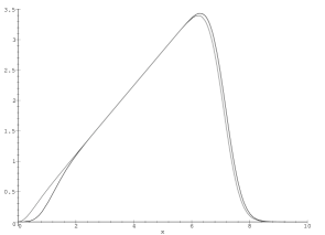
Figure 1: The charge fluctuation $(\Delta Q(R))^{2}$ for a system with 50 electrons and filling factor $m=1$. The two curves show the fluctuations of the ground state and of the state for one quasi-hole.

It is a non-trivial problem to construct a local charge operator which is insensitive to the background fluctuations of the ground state. In the context of a one-dimensional fermi system with fractionally charged solitons, the problem was solved by Kivelson and Schrieffer [8] and Bell and Rajaraman [9] who defined a charge operator using a smooth spatial cutoff. However, in 2 (and higher) dimensions this is not sufficient, also a cutoff in energy is needed, as discussed by Goldhaber and Kivelson [10]. In principle such a definition could be used also for the fractional quantum Hall states, however to implement this in the form of an explicitly defined charge operator seems difficult.

In this paper we have not made any attempt to introduce such a redefined charge operator. Instead we have used, as the relevant measure of the sharpness of a localized charge, the subtracted quantity

$$D(R)\equiv\Delta Q(R)-\Delta Q_{0}(R)\ \ \ \ \ ,$$ (7)

where $\Delta Q_{0}(R)$ is the fluctuation of the ground state. Each of the two terms in this expression are finite, and the difference is therefore well defined. The use of this expression is based on the intuitive idea that if an excited state can be characterized by a sharply defined, localized charge, that means that the charge fluctuation rapidly approaches the ground state value when the integration area $A$ is extended outside the region which characterizes the size of the excitation. In fact, it seems reasonable to assume that if the fluctuation vanishes for any reasonably defined local charge operator, then also the simple difference (7) will vanish. The only problem with the approach used here is of numerical character. The fluctuation will be a small number calculated as the difference between large numbers, and this put strong limits on the accuracy of the numerical calculations.

For the sake of illustration we show in Fig. 2 the charge expectation value and the charge fluctuation, with such a subtraction included, for the special case of a Laughlin quasi-hole at the integer filling factor $1$. In this case all the quantities needed in order to calculate the functions $C(R)$ and $D(R)$ can be found analytically, and we show the results for a system of 50 electrons. The excess charge, here negative, exponentially builds up to the plateau value $(-1)$ as $R$ increases from zero, and the charge fluctuations vanish once the plateau is reached. We also see edge effects at the droplet boundary $R\approx 7.1$. The figures clearly show that our definitions in Eqs. (2) and (7) reveal the basic properties of interest.

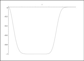
(a) $C_{\rm h}(R)$.

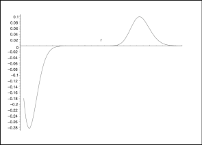
(b) $D_{\rm h}(R)$.

Figure 2: Quasi-hole charge $C_{\rm h}(R)$ and charge fluctuation $D_{\rm h}(R)$ for a system with 50 electrons and filling fraction $1/m=1$.

Before concluding this section on general definitions and relations, we shall introduce a quantity that will be very useful in the coming calculations. Consider

$${\hat{F}}(R)=\int_{A}{\rm d}^{2}\!u{\rm d}^{2}\!v{\hat{\rho}}_{2}(u,v),$$ (8)

where ${\hat{\rho}}_{2}(u,v)$ is the diagonal two-electron density operator. Using

$${\hat{\rho}}(u){\hat{\rho}}(v)={\hat{\rho}}_{2}(u,v)+\delta(u-v){\hat{\rho}}(u,v)$$ (9)

we can then express the fluctuation of the operator ${\hat{Q}}$ as

$$(\Delta Q(R))^{2} = \langle{\hat{Q}}^{2}(R)\rangle-\langle{\hat{Q}}(R)\rangle^{2}$$ (10)

$$= Q(R)+F(R)-(Q(R))^{2}.$$ (11)

The functions $Q,F$ are expectation values of ${\hat{Q}},{\hat{F}}$ in the specific state. In terms of the $N$-electron normalized wave function for the state they are

$$Q(R)=N\int_{A}d^{2}\!u\int d^{2}\!z_{2}\cdots d^{2}\!z_{N}\mid\psi(u,z_{2},\cdots,z_{N})\mid^{2}$$ (12)

$$F(R)=N(N-1)\int_{A}d^{2}\!ud^{2}\!v\int d^{2}\!z_{3}\cdots d^{2}\!z_{N}\mid\psi(u,v,z_{3},\cdots,z_{N})\mid^{2}$$ (13)

The expression (11) will be used when investigating the charge fluctuations of the Laughlin quasi-electrons, whereas (10) will be used in the case of Laughlin’s ground state and quasi-hole state as well as for Jain’s quasi-electrons.

3 Numerical methods to compute $Q$ and $\Delta Q$

3.1 General introduction

In all our computations we have used Monte Carlo integration with importance sampling according to the Metropolis algorithm [11, 12], and a brief discussion of some points of special importance for our calculations are given in appendix A. The specific probability distribution used to generate electron configurations varied from case to case. Each of them will be given in the sections following below, where we give descriptions of our methods that are detailed enough to allow the calculations to be reproduced.

Notice that in order to find the quasi-particle charge fluctuation $D(R)$ we need to find the two numbers $\Delta Q(R)$ and $\Delta Q_{0}(R)$, and then the difference between them. In general, this difference is very small compared to the numbers themselves. Since our aim is to decide if the difference is significantly different from zero, both $\Delta Q(R)$ and $\Delta Q_{0}(R)$ must be known with great precision. This is itself a challenging problem since each of them in turn is found from a difference between the numbers $\langle{\hat{Q}}^{2}(R)\rangle$ and $\langle{\hat{Q}}(R)\rangle^{2}$ which are large for large $R$. For all examined cases except for Laughlin’s quasi-electrons, this problem has been solved by evaluating $\langle{\hat{Q}}^{2}\rangle$ and $\langle{\hat{Q}}\rangle^{2}$ simultaneously, and benefit from the fact that the statistical errors then are correlated and tend to cancel. For the Laughlin quasi-electrons this method is inappropriate. Instead we have found values for $Q$ and $F$ defined in Eqs. (12) and (13). In the following discussion we will use the subscripts “h, Le” and “Je” to refer to quasi-holes, Laughlin quasi-electron and Jain quasi-electrons, respectively. The subscript “$0$” refers to the ground state.

3.2 The Laughlin ground state and quasi-hole state

The definitions (2) and (7) of the charge and charge fluctuations for the quasi-particle, require knowledge of the mean value and fluctuations of the ground state charge. For $N$ electrons at filling fraction $1/m$ the ground state is given by Laughlin’s wave function

$$\psi_{0}(z_{1},\cdots z_{N}^{*})=e^{-\frac{1}{2}\sum_{i=1}^{N}\mid z_{i}\mid^{2}}\prod_{k<l}(z_{k}-z_{l})^{m},$$ (14)

This describes an electron droplet with uniform particle density (in the bulk) and a radius approximately $\sqrt{mN}$ [12, 13]. In this case the numerical computations are simple. We use the true electron density to generate the electron configurations $(z_{1\alpha},\cdots,z_{N\alpha})$, that is we generate events according to the probability density,

$$p_{0}(z_{1},\cdots z_{N}^{*})=\frac{1}{I_{0}}|\psi_{0}(z_{1},\cdots z_{N}^{*})|^{2},$$ (15)

where

$$I_{0}=\int{\rm d}^{2N}\!z\,|\psi_{0}(z_{1},\cdots z_{N}^{*})|^{2}$$ (16)

is the normalization integral. For each specific configuration $\alpha$ the charge $Q_{\alpha}$ inside the area $A=\pi R^{2}$ is found simply by counting the $z$:s that satisfy $|z|\leq R$. From $n$ configurations the expectation values of ${\hat{Q}}(R)$ and ${\hat{Q}}^{2}(R)$ are estimated (simultaneously) by

$$\langle 0|{\hat{Q}}(R)|0\rangle=\frac{1}{n}\sum_{\alpha=1}^{n}Q_{\alpha},\hskip 28.45274pt\langle 0|{\hat{Q}}^{2}(R)|0\rangle=\frac{1}{n}\sum_{\alpha=1}^{n}Q_{\alpha}^{2},$$ (17)

and the ground state fluctuation $\Delta Q_{0}(R)$ is then found using Eq. (10).

The same method can also be used for a Laughlin quasi-hole, which is given by the wave function

$$\psi_{\rm h}(z_{1},\cdots z_{N}^{*})=e^{-\frac{1}{2}\sum_{i=1}^{N}\mid z_{i}\mid^{2}}\prod_{k<l}(z_{k}-z_{l})^{m}\prod_{i=1}(z_{i}-z_{0})\ \ \ \ \ .$$ (18)

This expression describes an electron droplet with an electron density which is the same as in the ground state, except for a small depleted region around the point $z_{0}$, the position of the quasi-hole [12]. Again we choose the probability distribution used to generate electron configurations to be the (normalized) electron probability density itself;

$$p_{\rm h}(z_{1},\cdots z_{N}^{*})=\frac{1}{I_{\rm h}}|\psi_{\rm h}(z_{1},\cdots z_{N}^{*})|^{2},\hskip 14.22636pt{\rm where}\hskip 8.53581ptI_{\rm h}=\int{\rm d}^{2N}\!z\,|\psi_{\rm h}(z_{1},\cdots z_{N}^{*})|^{2}.$$ (19)

For $z_{0}=0$ the expectation values $\langle{\rm h}|{\hat{Q}}(R)|{\rm h}\rangle$ and $\langle{\rm h}|{\hat{Q}}^{2}(R)|{\rm h}\rangle$ are then estimated, using the procedure described above.

3.3 The Laughlin quasi-electron state

The simple numerical method described above can not be used in the case of a Laughlin quasi-electron. The reason for this can immediately be seen from the wave function, which reads

$$\psi_{\rm Le}(z_{1},\cdots z_{N}^{*})=e^{-\frac{1}{2}\sum_{j=1}^{N}|z_{j}|}\prod_{i=1}^{N}(\partial_{z_{i}}-z_{0}^{*})\prod_{k<l}(z_{k}-z_{l})^{m}.$$ (20)

In this case the wave function contains derivatives, and these must be evaluated analytically before the expressions can be used in a computer program. Although in principle straightforward, we know of no efficient way of doing this for sufficiently many electrons.

To avoid this problem, we have considered two different methods for computing the charge and charge fluctuations of a Laughlin quasi-electron. The first uses “brute force”, and the numerical convergence is slow, although much better for small than for large $R$. The second method converges faster, and is best fitted for the bulk. Hence, the domains of validity of the two methods are complementary, which allows us to calculate for the whole range of $R$. Also there is some overlap where we can check against one another the results obtained by use of the two methods.

Method 1

We will here present the method most appropriate for small $R$. Consider then the expectation value of the charge operator when the quasi-electron is put at the origin;

$$Q_{\rm Le}(R)=\langle{\rm Le}|{\hat{Q}}(R)|{\rm Le}\rangle$$ (21)

$$= \frac{N}{I_{\rm Le}}\int_{A}{\rm d}^{2}\!z_{1}\int{\rm d}^{2(N-1)}\!z\,|\psi_{\rm Le}(z_{1},\cdots,z_{N}^{*})|^{2}$$ (22)

$$= \frac{N}{I_{\rm Le}}\int_{A}{\rm d}^{2}\!z_{1}\int{\rm d}^{2(N-1)}\!z\,e^{-\sum_{i=1}^{N}\mid z_{i}\mid^{2}}\prod_{k<l}\mid z_{k}-z_{l}\mid^{2m}\prod_{j=2}^{N}(\mid z_{j}\mid^{2}-1)\mid\sum_{i=2}^{N}\frac{m}{z_{1}-z_{i}}\mid^{2}$$ (23)

$$= \frac{N}{I_{\rm Le}}\int_{A}{\rm d}^{2}\!z_{1}\int{\rm d}^{2(N-1)}\!z\,p^{\prime}_{\rm Le}(z_{1},\cdots,z_{N}^{*})$$ (24)

where $I_{\rm Le}$ is the normalization integral, and $p^{\prime}_{\rm Le}$ is the integrand in Eq. (23). The expression in Eq. (23) is obtained by partially integrating the coordinates $z_{2},\cdots,z_{N}$, but differentiating the VanderMonde determinant directly with respect to $z_{1}$, which is integrated over the finite area $A$. We emphasize that $p^{\prime}_{\rm Le}$ is not the true electron density of the system, in fact, since it takes on negative as well as positive value, it cannot be taken as a probability density. Nevertheless, the normalization integral $I_{\rm Le}$ can be expressed in terms of $p^{\prime}_{\rm Le}$,

$$I_{\rm Le}=\int{\rm d}^{2N}\!z\,|\psi_{\rm Le}(z_{1},\cdots,z_{N}^{*})|^{2}=\int{\rm d}^{2N}\!z\,p^{\prime}_{\rm Le}(z_{1},\cdots,z_{N}^{*})\ \ \ \ \ ,$$ (25)

and this enables us to write,

$$Q_{\rm Le}(R)=N\frac{\int_{A}{\rm d}^{2}\!z_{1}\int{\rm d}^{2(N-1)}\!z\,p^{\prime}_{\rm Le}(z,z^{*})}{\int{\rm d}^{2N}\!z\,p^{\prime}_{\rm Le}(z,z^{*})}=N\frac{\int_{A}{\rm d}^{2}\!z_{1}\int{\rm d}^{2(N-1)}\!z\,|p^{\prime}_{\rm Le}(z,z^{*})|\,{\rm sgn}(p^{\prime}_{\rm Le})}{\int{\rm d}^{2N}\!z\,|p^{\prime}_{\rm Le}(z,z^{*})|\,{\rm sgn}(p^{\prime}_{\rm Le})}\ \ \ ,$$ (26)

where ${\rm sgn}(p^{\prime}_{\rm Le})$ is the sign function. Eq. (26) tells us that if the electron coordinates are generated according to the absolute value $|p^{\prime}_{\rm Le}(z,z^{*})|$ then the expectation value $Q_{\rm Le}(R)$ can be estimated as the ratio between the Monte Carlo expectation values of $S(R-|z_{1}|)\,{\rm sgn}(p^{\prime}_{\rm Le})$ and ${\rm sgn}(p^{\prime}_{\rm Le})$, where $S(x)$ is $1$ when $x\geq 0$ and $0$ otherwise. In practice we thus do as follows: For each electron configuration $\alpha$ determine whether particle $1$ is inside $R$. If it is, set $t_{\alpha}=\pm 1$ according to the sign of $p^{\prime}_{\rm Le}(z,z^{*})$. Otherwise set $t_{\alpha}=0$. Independent of the position of $z_{1}$ set $n_{\alpha}=\pm 1$ according to the sign of $p^{\prime}_{\rm Le}$. The expectation value is then found by

$$Q_{\rm Le}(R)=\frac{\sum_{\alpha=1}^{n}t_{\alpha}}{\sum_{\alpha=1}^{n}n_{\alpha}}.$$ (27)

Notice that the function $|p^{\prime}_{\rm Le}(z,z^{*})|$ is not symmetric in all variables since it treats $z_{1}$ in a special way. This implies that the numerical convergence rate is $N$ times slower than it would have been if we could use a symmetric function, everything else being equal.

Since the electron coordinates were not generated according to the true electron density, the expectation value $\langle{\hat{Q}}^{2}(R)\rangle$ can not be found using the simple method described for the Laughlin ground state and quasi-hole. Instead we turn to Eq. (11) and compute

$$F_{\rm Le}(R)=\langle{\rm Le}|{\hat{F}}(R)|{\rm Le}\rangle$$ (28)

$$= \frac{N(N-1)}{I_{\rm Le}}\int_{A}{\rm d}^{2}\!z_{1}{\rm d}^{2}\!z_{2}\int{\rm d}^{2(N-2)}\!z\,|\psi_{\rm Le}(z_{1},\cdots,z_{N}^{*})|^{2}$$ (29)

$$= \frac{N(N-1)}{I_{\rm Le}}\int_{A}{\rm d}^{2}\!z_{1}{\rm d}^{2}\!z_{2}\int{\rm d}^{2(N-2)}\!z\,e^{-\sum_{i=1}^{N}|z_{i}|^{2}}\prod_{k<l}|z_{k}-z_{l}|^{2m}\prod_{k=3}^{N}(|z_{k}|^{2}-1)$$ (31)

$$\hskip 113.81102pt\times|\sum_{i\neq 1}^{N}\frac{m}{z_{1}-z_{i}}\sum_{j\neq 2}^{N}\frac{m}{z_{2}-z_{j}}+\frac{m}{(z_{1}-z_{2})^{2}}|^{2}.$$

The VanderMonde determinant has now been differentiated with respect to both $z_{1}$ and $z_{2}$, while the other coordinates were integrated by parts. The integrand in Eq. (31) is more complicated than $p^{\prime}_{\rm Le}$ in Eq. (24). However, if we now define $p^{\prime}_{\rm Le}$ to be the integrand of Eq. (31), then the normalization integral $I_{\rm Le}$ can still be expressed as $I_{\rm Le}=\int{\rm d}^{2N}\!z\,p^{\prime}_{\rm Le}(z,z^{*})$, and the value of $F_{\rm Le}(R)$ be estimated as the ratio between two Monte Carlo estimates, analogously to the method above. Notice that in the present case the function $|p^{\prime}_{\rm Le}(z,z^{*})|$ treats two coordinates differently from the others. The convergence rate of this non-symmetric treatment will be $N(N-1)$ times slower than a symmetric one, again everything else being equal.

The slow convergences for large $N$ that we have referred to, imply problems for the numerical calculations discussed here. Nevertheless, for small values of $R$ we do obtain well converged results. These can be used as a complement to the bulk results found by use of the method of the next section. In addition, the ranges of validity of the two methods do have some overlap, and we hence check the results against one another. We also hope that the treatment of “negative probability densities” is instructive, and would like to mention that also Ref. [13] contains a discussion of this topic. It will be used again in the next section.

Method 2

This section presents a method that improves Method 1 in two important ways: First, a function symmetric in all electron coordinates is used to generate configurations, and thus we achieve a huge improvement in the convergence rate. Second, the same electron configurations are now used for calculating both $Q_{\rm Le}(R)$ and $F_{\rm Le}(R)$. However, to determine the functions we need to use numerical derivatives in addition to the Monte Carlo integration.

Define the quantity

$${\tilde{p}}_{\rm Le}(z_{1},\cdots,z_{N}^{*})=e^{-\sum_{i=1}^{N}|z_{i}|^{2}}\prod_{j=1}^{N}(|z_{j}|^{2}-1)\prod_{k<l}|z_{k}-z_{l}|^{2m}.$$ (32)

Of course, ${\tilde{p}}_{\rm Le}$ is nothing else than the integrand appearing if we use integration by parts to all coordinates in Eqs. (22, 29), and it is clear that

$$I_{\rm Le}=\int{\rm d}^{2N}\!z\,|\psi_{\rm Le}(z_{1},\cdots,z_{N}^{*})|^{2}=\int{\rm d}^{2N}\!z\,{\tilde{p}}_{\rm Le}(z_{1},\cdots,z_{N}^{*}).$$ (33)

In addition, define the auxiliary functions,

$${\widetilde{Q}}(R)=\frac{N}{I_{\rm Le}}\int_{A}{\rm d}^{2}z_{1}\int{\rm d}^{2(N-1)}z\,{\tilde{p}}_{\rm Le}(z_{1},\cdots,z_{N}^{*}),$$ (34)

$${\widetilde{F}}(R_{1},R_{2})=\frac{N(N-1)}{I_{\rm Le}}\int_{A_{1}}{\rm d}^{2}z_{1}\int_{A_{2}}{\rm d}^{2}z_{2}\int{\rm d}^{2(N-2)}z\,{\tilde{p}}_{\rm Le}(z_{1},\cdots,z_{N}^{*}).$$ (35)

Notice that the areas $A_{1}$ and $A_{2}$ in general are different.

The auxiliary functions ${\widetilde{Q}}(R)$ and ${\widetilde{F}}(R_{1},R_{2})$ are closely related to the functions, $Q_{\rm Le}(R)$ and $F_{\rm Le}(R)$ that we want to compute. When partial integration is applied to the variable $z_{1}$, boundary terms will appear since the integration area $A$ covers only a part of the full droplet. The boundary terms can be expressed in terms of ${\widetilde{Q}}(R)$ and ${\widetilde{F}}(R_{1},R_{2})$ and their first two derivatives and give the relations

$$Q_{\rm Le}(R) = {\widetilde{Q}}(R)+c_{1}(R)\frac{{\rm d}{\widetilde{Q}}(R)}{{\rm d}R}+c_{2}(R)\frac{{\rm d}^{2}{\widetilde{Q}}(R)}{{\rm d}R^{2}},$$ (36)

$$F_{\rm Le}(R) = {\widetilde{F}}(R,R)+c_{1}(R)\left(\frac{\partial{\widetilde{F}}}{\partial R_{1}}+\frac{\partial{\widetilde{F}}}{\partial R_{2}}\right)_{R}$$ (37)

$$+c_{2}(R)\left(\frac{\partial^{2}{\widetilde{F}}}{\partial R_{1}^{2}}+\frac{\partial^{2}{\widetilde{F}}}{\partial R_{2}^{2}}\right)_{R}+c_{1}^{2}(R)\left(\frac{\partial^{2}{\widetilde{F}}}{\partial R_{1}R_{2}}\right)_{R}$$

$$+c_{1}(R)c_{2}(R)\left(\frac{\partial^{3}{\widetilde{F}}}{\partial R_{1}^{2}R_{2}}+\frac{\partial^{3}{\widetilde{F}}}{\partial R_{1}R_{2}^{2}}\right)_{R}+c_{2}^{2}(R)\left(\frac{\partial^{4}{\widetilde{F}}}{\partial R_{1}^{2}R_{2}^{2}}\right)_{R}.$$

The subscript $R$ means that both $R_{1}$ and $R_{2}$ should be set equal to $R$ after differentiating. Eqs. (36) and (37) are exact equalities, and the derivations are shown in appendix B. We have used the notation

$$c_{1}(R)=\frac{4R^{4}-7R^{2}+1}{4R(R^{2}-1)^{2}}, c_{2}(R)=\frac{1}{4(R^{2}-1)}.$$ (38)

The numerical method for obtaining $Q_{\rm Le}(R)$ and $F_{\rm Le}(R)$ is as follows: First generate coordinates according to the absolute value $|{\tilde{p}}_{\rm Le}|$, and estimate ${\widetilde{Q}}(R)$ and ${\widetilde{F}}(R_{1},R_{2})$ simultaneously in the way described above, but now with the advantage of having a generating function that is symmetric in the electron coordinates. The computation is done for $R,R_{1},R_{2}=hk$ where $h$ is a fixed grid spacing and $k=0,1,\cdots,K$. The maximum value $K$ is taken large enough that the radii take values larger than the radius of the electron droplet, which for $N$ electrons at filling fraction $1/m$ is $\sqrt{mN}$. From the resulting one- and two-dimensional grid of data we estimate the derivatives by the formula

$$\frac{{\rm d}{\widetilde{Q}}(R)}{{\rm d}R}\approx\frac{1}{2h}({\widetilde{Q}}(R+h)-{\widetilde{Q}}(R-h))$$ (39)

with similar expressions for higher derivatives. The values for $Q_{\rm Le}(R)$ and $F_{\rm Le}(R)$ are found by use of Eqs. (36) and (37), and the value of $\Delta Q_{\rm Le}(R)$ by use of Eq. (11). In the computation we have used the two step sizes $h=0.1$ and $h=0.2$, and as will be discussed in detail in section 4, we have sufficient control over the errors introduced by the discrete differentiation.

3.4 The Jain quasi-electron

We have also computed the charge and charge fluctuations for the wave function defined by Jain. The wave function has the form [4]

$$\psi_{\rm Je} = {\cal P}e^{-\frac{1}{2}\sum_{i=1}^{N}|z_{i}|^{2}}\left|\begin{array}[]{cccc}z_{1}^{*}&z_{2}^{*}&\cdots&z_{N}^{*}\\ 1&1&\cdots&1\\ z_{1}&z_{2}&\cdots&z_{N}\\ \vdots&\vdots&\vdots&\vdots\\ z_{1}^{N-2}&z_{2}^{N-2}&\cdots&z_{N}^{N-2}\end{array}\right|\prod_{k<l}(z_{k}-z_{l})^{m-1}$$ (45)

$$= {\cal P}e^{-\frac{1}{2}\sum_{i=1}^{N}|z_{i}|^{2}}\prod_{k<l}(z_{k}-z_{l})^{m-1}\sum_{j=1}^{N}\left(z_{j}^{*}(-1)^{j}\prod_{k<l;k,l\neq j}(z_{k}-z_{l})\right)$$ (46)

$$= {\cal P}e^{-\frac{1}{2}\sum_{i=1}^{N}|z_{i}|^{2}}\sum_{j=1}^{N}\left(z_{j}^{*}\frac{1}{\prod_{i\neq j}(z_{j}-z_{i})}\right)\prod_{k<l}(z_{k}-z_{l})^{m}.$$ (47)

Here ${\cal P}$ means projection onto the lowest Landau level. The importance of this projection has been studied [15], and it turns out that even without ${\cal P}$ most of the wave function is already in the lowest Landau level. Our calculations, which are performed for the unprojected as well as the projected state, give results that are in accordance with this.

Following the general scheme for projection onto the lowest Landau level [16], we let $z_{j}^{*}\rightarrow\partial_{z_{j}}$ with the differentiation operator acting on everything except the exponential factor $e^{-\frac{1}{2}\sum_{i=1}|z_{i}|^{2}}$. This yields

$$\psi_{\rm Je}=e^{-\frac{1}{2}\sum_{i=1}^{N}|z_{i}|^{2}}\prod_{k<l}(z_{k}-z_{l})^{m}\sum_{j=1}^{N}\frac{1}{\prod_{i\neq j}(z_{j}-z_{i})}\left(-\sum_{k\neq j}\frac{1}{(z_{j}-z_{k})}+\frac{m}{\sum_{k\neq j}(z_{j}-z_{k})}\right).$$ (48)

This expression is symmetric in all coordinates. In addition, the squared absolute value is the true electron density in the system, so in order to find $Q_{\rm Je}(R)$ and $\Delta Q_{\rm Je}(R)$ we can simply adopt the method used for the Laughlin ground state and quasi-hole state, Eq. (17), now with $p_{\rm Je}=|\psi_{\rm Je}|^{2}/I_{\rm Je}$ as the probability distribution used in the Metropolis algorithm. For the unprojected state the method is of course similar, and the expression in Eq. (47), now without the projection operator ${\cal P}$, is used for $p_{\rm Je}$.

4 Results of charge mean value and charge fluctuation computations

This section presents the results following from the calculations described in the previous section. For $m=3$, i.e. for filling fraction $1/3$ of the lowest Landau level, we have calculated charge and charge fluctuations in the cases of a Laughlin quasi-hole, a Laughlin quasi-electron and a Jain quasi-electron. In all three cases the quasi-particle has been located at the center of a circular electron droplet. For the quasi-hole we have made calculations for electron droplets consisting of 50 and 100 particles. Systems with 50, 100 and 200 electrons were considered in the case of a Laughlin quasi-electron, whereas we did calculations for 50 electrons with the Jain quasi-electron in the system. We find that for all quasi-particles the numerical calculations reproduce well the expected bulk values of the charge mean values. There are finite-size effects, due to the limited number of electrons, which are most dominant for 50 electrons in the case of the Laughlin quasi-electron. However, these effects are constrained to the regions close to the position of the quasi-particle and to the edge of the electron droplet. For $100$ and $200$ electrons (and even for $50$ electrons in the case of a quasi-hole or a Jain quasi-particle) the bulk values, $-1/3$ for quasi-holes and $+1/3$ for quasi-electrons, are reproduced within small statistical errors. Charge is then measured in units of the electron charge. For the quasi-hole and Jain quasi-electron the calculations reproduce, again within small statistical errors, the expected bulk value zero for the charge fluctuations. However, for the Laughlin quasi-electron we find larger fluctuations than in the other two cases. At an absolute scale they are small, but they are significantly different from zero within the small errors of the calculation.

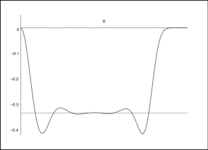
Figure 3: Quasi-hole charge $C_{\rm h}(R)$ for systems with 50 and 100 electrons. The horizontal line is $-1/3$.

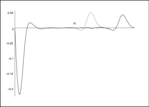
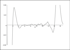
Figure 4: (a): Quasi-hole charge fluctuations $D_{\rm h}(R)$ for systems with 50 and 100 electrons. (b): Enlarged vertical axis emphasizing the bulk behaviour of $D_{\rm h}(R)$ for 100 electrons.

Fig. 3 shows the $R$-dependence of the quasi-hole charge $C_{\rm h}(R)$, for system sizes of 50 and 100 electrons. The figure shows that there are three distinct regions. For small $R$ there is a region where the charge builds up when $R$ increases, which we clearly may identify with the location of the quasi-particle. There is an intermediate region where the charge seems to stabilize at a constant value, which is consistent with the expected bulk value $-1/3$ for the quasi-hole charge. For larger $R$ there is a region where the charge again decreases to zero, and this we identify with the edge region of the droplet. The charge profile of the quasi-hole, for small $R$, is essentially identical for $50$ and $100$ electrons, and that is also the case for the charge profile at the edge. The main difference between the two cases is the size of the intermediate region, the bulk region of the electron droplet.

The distinction between the three regions for $m=3$ is similar to what is seen in Fig. 2a for $m=1$ . The main difference is the presence of oscillations for $m=3$, in the charge profile for small and large $R$, which to some extent extends into the intermediate region. These oscillations are of the same form as has previously been found in numerical calculations of the charge density of Laughlin quasi-particles [13].

In Fig. 4 the charge fluctuations $D_{\rm h}(R)$ of the Laughlin quasi-hole are shown. Figure (a) compares the results obtained for systems with 50 and 100 electrons, whereas figure (b) shows an enlarged picture of the 100 electron case. The irregularities of the curve seen here are presumably due to the statistical fluctuations in the Monte-Carlo calculations and they give an indication of the size of these statistical errors. The results shown in Fig. 4 confirms the picture that the effect of the quasi-hole is restricted to a limited region around the origin. In the bulk of the electron droplet the charge fluctuations vanish within small statistical errors, whereas there are substantial fluctuations in the charge inside the quasi-hole and at the edge. According to the discussion in section 2, this is consistent with the assumption that the charge of the Laughlin quasi-hole is a sharply defined quantum number.

The results presented so far are obtained for a discrete set of $R$-values, $R=hk$ with $h=0.2$ and $k=0,1,\cdots,K$. The maximum number $K$ is chosen such that $hK$ is larger than the radius $\sqrt{mN}$ of the electron droplet. Recall that lengths are measured in units of $\sqrt{2}\ell_{B}$, with $\ell_{B}$ as the magnetic length. The ground state data are for the case of 50 electrons obtained from 45 million electron configurations, and for 100 electrons from 17 million configurations. All quasi-hole data are found from 10 million configurations. For each data set we have numerically estimated the standard deviation of the considered mean value. This enables us to estimate the numerical errors in the differences $C_{\rm h}(R)=Q_{\rm h}(R)-Q_{\rm 0}(R)$ and $D_{\rm h}(R)=\Delta Q_{\rm h}(R)-\Delta Q_{\rm 0}(R)$ as well. Table 1 shows some of the expectation values along with the computed statistical errors in the case of 50 electrons. The results are consistent with a quasi-hole charge that has the bulk value $-1/3$ and vanishing charge fluctuations. The estimated values for the standard deviation are somewhat larger than the irregularities of the plotted curve shown in Fig. 4.

$R$	$C_{\rm h}(R)$	$D_{\rm h}(R)$
$4.0$	$-0.3219\pm 0.0003$	$-0.0028\pm 0.002$
$6.0$	$-0.3334\pm 0.0004$	$+0.0003\pm 0.005$
$8.0$	$-0.3371\pm 0.0005$	$+0.0000\pm 0.008$
$10.0$	$-0.3345\pm 0.0005$	$-0.0044\pm 0.013$

Table 1: Charge $C_{\rm h}$ and charge fluctuations $D_{\rm h}$ for the Laughlin quasi-hole in the case of 50 electrons. Both mean values and estimated errors are listed. The quantities $Q_{\rm h}$ and $\Delta Q_{\rm h}$ were obtained from 10 million electron configurations, while 45 million configurations were used to find $Q_{0}$ and $\Delta Q_{0}$.

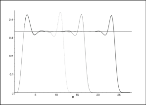
Figure 5: Charge $C_{\rm Le}(R)$ of a Laughlin quasi-electron. For $0\leq R\leq 2.4$ the curve is obtained by using Method 1 of section 3.3 for a system with 50 electrons. For $R\geq 2.4$ Method 2 was used, and the curves are for 50, 100 and 200 electrons. The horizontal line is $1/3$.

We will now turn to the case of a Laughlin quasi-electron located at the origin, and we consider first Fig. 5 where the charge $C_{\rm Le}(R)$ is displayed. For $R\leq 2.4$ the curve is found for a system with 50 electrons using Method 1 of the previous section. The three different curves for $R\geq 2.4$ are for 50, 100 and 200 electrons and are found using Method 2. We observe again that there is a well defined region where the value of the charge is almost constant and agrees with the expected bulk value of $1/3$ for the integrated quasi-electron charge. A more detailed presentation of the results show that for $100$ and $200$ electrons this is indeed the case within the small errors of the calculation (to be discussed below) whereas for $50$ electrons there is a small deviation which we assume to be a finite-size effect (see Fig. 7). Comparing with Fig. 3 we see that the curves for $C_{\rm Le}(R)$ are, apart from a sign, similar to the curves obtained for the quasi-hole.

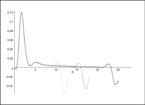
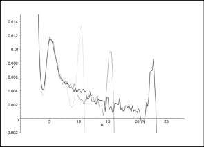
Figure 6: Laughlin quasi-electron charge fluctuations $D_{\rm Le}(R)$. The single curve for $0\leq R\leq 2.4$ is found by using Method 1 of section 3.3 in a system with 50 electrons. The three curves for $R\geq 2.4$ are for 50, 100 and 200 electrons, and Method 2 was used.

Fig. 6 presents the calculated values of the charge fluctuations $D_{\rm Le}(R)$ of the Laughlin quasi-electron. (Also here the single curve shown for $R\leq 2.4$ is obtained for a system of 50 electrons with the use of Method 1, and for $R\geq 2.4$ the three curves are obtained for systems of 50, 100 and 200 electrons with the use of Method 2.) Figure (b) is an enlarged version of figure (a), now without the small $R$ dependence. We observe that for the system sizes considered here, there are surviving fluctuations for the whole range of $R$-values inside the electron droplet. This result is seen most clearly in Fig. 6b, where the irregularities indicate the size of the statistical fluctuations in the computation. A further discussion of uncertainties in the result will follow below.

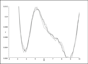
(a) $D_{\rm Le}(R)$.

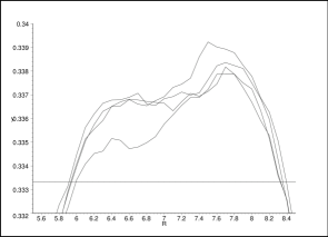
(b) $C_{\rm Le}(R)$.

Figure 7: Four statistically independent curves for the charge fluctuations $D_{\rm Le}(R)$, (a), and the charge $C_{\rm Le}(R)$, (b) of a Laughlin quasi-electron. Each curve is based on approximately $48$ million configurations for the quasi-electron data. The same ground state data, found from 125 million configurations, were used in all four cases. The lattice constant is $h=0.1$

The behaviour of the charge fluctuation curve for the Laughlin quasi-electron is clearly different from that of the quasi-hole, which is shown in Fig. 4. For a system of $100$ electrons the quasi-hole charge fluctuations were seen to vanish in the bulk, within the small statistical errors of the calculations. A comparison between Figs. 6b and 4b, with compensation for the difference in vertical scale, emphasizes the difference between the two cases. We thus conclude that there are charge fluctuations for the Laughlin quasi-electron that are larger and extend much further out than they do for the quasi-hole. Even though the expectation value of the quasi-electron charge is well defined and agrees with the expected bulk value (within the statistical uncertainty) in an intermediate interval of $R$, there are small but non-vanishing charge fluctuations which persist also here. In this sense the charge is not a sharply defined quantum number for the quasi-electron. However, there is a slow decay in the fluctuation curve for increasing $R$, and we cannot rule out that for even larger systems, with electron numbers $N>200$, the value of the charge fluctuation will settle at the value zero further out in the bulk of the electron droplet. If that is the case, the quasi-electron charge is a sharp quantum number, but the size of the quasi-electron, as measured through these fluctuations, will be much larger than the size estimated from the charge expectation value or found by comparison with the charge fluctuations of the quasi-hole.

The curves shown here for $R\geq 2.4$ are based on the following number of electron configurations: To find the quantities $Q_{\rm Le}(R)$ and $\Delta Q_{\rm Le}(R)$ we used 191 million configurations in the case of 50 electrons, 42 million for 100 electrons and 102 million for 200 electrons. The ground state quantities $Q_{0}(R)$ and $\Delta Q_{0}(R)$ were obtained from 125 million configurations for 50 electrons, 17 million for 100 electrons and 86 million electron configurations in the case of 200 electrons. For $R\leq 2.4$ we used 4.4$\cdot$10⁹ electron configurations to find the quasi-electron quantities $Q_{\rm Le}(R)$ and $\Delta Q_{\rm Le}(R)$. The calculations were done for values of $R=hk$, with $k=0,1,\cdots,K$, and $h=0.1$ in the 50 electron case and $h=0.2$ for the two other system sizes. We would also like to mention that in the case of 50 electrons, for a small range of $R$ around $R=2.4$, both the calculation methods, Method 1 and Method 2, converged well and gave coinciding results for $C_{\rm Le}(R)$ and $D_{\rm Le}(R)$.

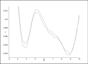
(a) $D_{\rm Le}(R)$.

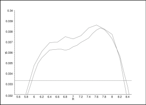
(b) $C_{\rm Le}(R)$.

Figure 8: Charge fluctuations $D_{\rm Le}(R)$, (a), and charge $C_{\rm Le}(R)$, (b), found from two different lattice spacings $h=0.1$ and $h=0.2$ in the case of 50 electrons.

The conclusion for the charge fluctuations suggested above is based on the assumption that the irregularities seen in the fluctuation curves give a measure of the errors introduced in the computation. However, in order to establish the conclusion more firmly, we have considered numerical errors more carefully. The errors include accidental errors due to statistical fluctuations in the numerically obtained mean values, as well as systematical errors due to the finite lattice spacing $h$ used in the numerical derivatives. Since the charge fluctuations, as well as the charge expectation values, have been calculated by a different method, which involves “negative probabilities”, the standard deviations of the calculated mean values are not so easily established, as in the case of the quasi-hole. In the case of the Laughlin quasi-electron the statistical errors therefore have been estimated simply by comparing the results of independent runs of the Monte-Carlo routine. To investigate the possible systematical errors we compare the results obtained by the use of two different step lengths and we compare the results of numerical differentiation with exact results, by applying the methods to a representative test function which can be handled analytically.

The estimate for the statistical errors is obtained by dividing the numerical data for ${\widetilde{Q}}(R)$ and ${\widetilde{F}}(R_{1},R_{2})$ into four statistically independent piles, each consisting of approximately $48$ million electron configurations. For each pile we have computed $C_{\rm Le}(R)$ and $D_{\rm Le}(R)$, using the same ground state data in all cases. Fig. 7a shows the four fluctuation curves found in this way for the case of $50$ electrons, while Fig. 7b shows the four independent charge curves. For a given $R$ we estimate the errors in the mean values as half the difference $(D_{\rm Le}(R))_{\rm max}-(D_{\rm Le}(R))_{\rm min}$, and similarly for $C_{\rm Le}(R)$. For the charge fluctuations this number is from the figure seen to typically take the value $0.0005$, and implies for example for $R=7$ that the mean value found is approximately $10$ times larger than this error. Fig. 7 also shows that the estimation of the errors obtained through the independent runs gives essentially the same results as the estimation obtained visually from the irregularities of a single curve. As judged from Fig. 6 the statistical errors for larger $R$, in the $100$ and $200$ electron curves, may be slightly larger than displayed by the $50$ electron curves. However, the value of the fluctuations still are significantly different from zero in most of the electron droplet.

A similarly estimated error in the charge expectation value $C_{\rm Le}(R)$ is approximately $0.001$. A detailed presentation (not included here) of the results in the cases of $100$ and $200$ electrons shows that the calculated charge expectation values do not deviate significantly (within this error) from $1/3$ in the bulk of the electron droplet.

(a) ${\widetilde{F}}(R_{1},R_{2})$

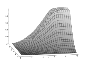
(b) $f_{1}(R_{1},R_{2})$

Figure 9: Comparison between (a): The Monte Carlo estimated function ${\widetilde{F}}(R_{1},R_{2})$ for 50 electrons and lattice spacing $h=0.2$, and (b): The analytically found test function $f_{1}(R_{1},R_{2})$ from Eq. (49), also calculated for 50 electrons. In both cases the factor $N(N-1)$ has been divided out.

We will now discuss the systematical errors introduced by the finite lattice spacing $h$. For small $h$ the lattice spacing will give errors in the numerical derivatives, Eqs. (36) and (37), which are proportional to $h^{2}$. The above results for 50 electrons are all found using $h=0.1$. In addition we have performed computations with $h=0.2$, and Fig. 8 compares curves for $D_{\rm Le}(R)$ and $C_{\rm Le}(R)$, obtained with these two values of $h$. We observe that the differences are similar in size to the statistical error that we have already considered. Due to the $h$-dependence of the error for small $h$ we expect that a further reduction in the lattice spacing will introduce differences which are smaller than the differences between the results obtained with $h=0.2$ and $h=0.1$. Results for $h=0.02$ seem to confirm this.

To make an independent check of the error introduced by the discrete differentiation, we have applied this operation to a test function with a similar form as ${\widetilde{F}}(R_{1},R_{2})$. From Eqs. (32), (35) and (14) we observe that, apart from the factor $\prod_{i=1}^{N}(|z_{i}|^{2}-1)$ the function ${\widetilde{F}}(R_{1},R_{2})$ is nothing else than the integrated two-particle density of the ground state for filling fraction $1/3$. We therefore expect that except for a scaling in distance, the function

$$f_{1}(R_{1},R_{2})=\frac{N(N-1)}{I_{1}}\int_{A_{1}}{\rm d}^{2}z_{1}\int_{A_{2}}{\rm d}^{2}z_{2}\int{\rm d}^{2(N-2)}z\ |\psi_{1}|^{2},$$ (49)

will mimic the main properties of the function ${\widetilde{F}}(R_{1},R_{2})$ reasonably well. Here $\psi_{1}$ is the wave function for the $m=1$ ground state (14), and $I_{1}$ is the corresponding normalization integral. That this anticipation is indeed fulfilled is seen in Fig. 9, where the analytically determined function $f_{1}(R_{1},R_{2})$ is compared to the numerically found function ${\widetilde{F}}(R_{1},R_{2})$. Both cases are for 50 electrons, and in each figure the surface starts from $0$ on the $R_{1}$ and $R_{2}$ axes, and then smoothly builds up to the value $N(N-1)$ as the edge of the electron droplet is reached. For the test function $f_{1}(R_{1},R_{2})$ we have then computed the right hand side of Eq. (37) in two ways: We have computed it analytically, and in addition we have calculated it by use of the discrete differentiation, Eq. (39), with lattice spacing $h=0.1$. We found errors in the result obtained with the discrete derivatives which were approximately $0.0005$ in the central part of the droplet. This agrees well with the results found from runs of the Monte Carlo routine with the two different spacings, $h=0.2$ and $h=0.1$, and are similar to the estimated value for the statistical errors.

Based on these estimates of the errors introduced in the computation we find it reasonable to conclude that the deviations from zero seen in Fig. 6 for the charge fluctuations are real and not due to the errors introduced by the calculations.

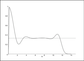
Figure 10: Charge $C_{\rm Je}(R)$ of a Jain quasi-electron in a system with 50 electrons. (a): Projected state, Eq. (48). (b): Unprojected state, Eq. (47).

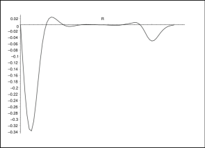
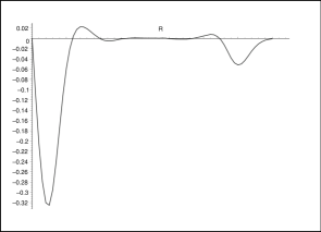
Figure 11: Charge fluctuations $D_{\rm Je}(R)$ of a Jain quasi-electron in a system with 50 electrons. (a): Projected state. (b): Unprojected state.

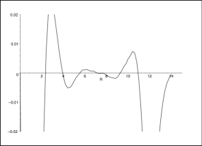
Figure 12: Fluctuations $D_{\rm Je}(R)$ of a Jain quasi-electron in a system with 50 electrons. (a): Projected state. (b): Unprojected state.

As noted above, we have also studied the charge and charge fluctuations for the quasi-electron defined by Jain’s wave function. This investigation was prompted by the behaviour found for the Laughlin quasi-electron, as a wish to compare the different proposals for the wave function. For a Jain quasi-electron located at the origin calculations have been performed for the projected state, Eq. (48), as well as for the unprojected state, Eq. (47). In both cases we have considered only a system of 50 electrons.

Fig. 10 compares the charge $C_{\rm Je}(R)$, as found for the projected state, to the corresponding quantity for the unprojected state, with the results for the projected one in the figure (a). We readily notice that there is almost no difference between the two figures, i.e. projection onto the lowest Landau level does not make any important difference in the present context. In both cases there is a well defined intermediate region where the curve is consistent with the expected integrated charge value $1/3$ (times the electron charge). When compared to Fig. 5 we notice that the amplitude of the peak for small $R$ is larger for the Jain quasi-electrons than it is for the Laughlin quasi-electrons, but apart from this the differences in charge expectation values are rather small for the two definitions of the quasi-electron wave function.

This similarity changes when we consider the charge fluctuations. For the Jain quasi-electron these are displayed in Fig. 11, and Fig. 12 shows the same results with the vertical axes enlarged. We observe again that the projection onto the lowest Landau level has a very small effect on the result. But the most compelling observation is that there exists a small region, which we interpret as corresponding to the bulk of the droplet, where the charge fluctuations are very small, indeed consistent with the value zero within small statistical errors (see the discussion below). The range of $R$ for which this is true is about the same as the range where the charge mean value, shown in Fig. 10, is close to the bulk value $1/3$. This behaviour is similar to the results we found for the Laughlin quasi-hole, and differs from what we saw for the Laughlin quasi-electron.

$R$	$C_{\rm Je}(R)$	$D_{\rm Je}(R)$
$4.0$	$0.3640\pm 0.0002$	$-0.001\pm 0.001$
$6.0$	$0.3281\pm 0.0002$	$+0.001\pm 0.003$
$8.0$	$0.3355\pm 0.0003$	$-0.001\pm 0.005$
$10.0$	$0.3383\pm 0.0003$	$+0.005\pm 0.007$

Table 2: Charge $C_{\rm Je}$ and charge fluctuations $D_{\rm Je}$ for the Jain quasi-electron in the case of 50 electrons. Both mean values and estimated errors are listed.

The results presented here are based on the following set of data: For the ground state we used 45 million electron configurations, whereas we for the Jain quasi-electrons used 77 million configurations for the projected state and 34 million for the unprojected. We have performed calculations for $R=hk$ with $h=0.2$ and $k=0,1\cdots,K$. For each set of data we estimated the numerical standard deviations in $C_{\rm Je}$ and $D_{\rm Je}$. Some of the results are listed in Table 2. The table shows, for the listed values of $R$, that the calculated values for both $C_{\rm Je}$ and $D_{\rm Je}$ are consistent with the expected bulk values within the estimated errors.

5 Statistics parameter of the Jain quasi-electrons

The studies of the charge fluctuations presented in this paper have been motivated by the results of Ref. [6], where the charge and statistics parameters of the Laughlin quasi-electrons were studied numerically, by Berry phase calculations, for systems of up to $200$ electrons. Whereas the expected charge value, in those calculations, was well reproduced, no stable value for the statistics parameter was found. This was clearly different from calculations of the statistics parameter of the quasi-hole. Our hypothesis has been that the discrepancy between the quasi-hole and quasi-electron results is due to more long range fluctuations in the correlation functions for the latter. This conclusion seems to be supported by the results of the charge fluctuation calculations presented in this paper.

The alternative definition of the quasi-electron wave function, given by Jain, seems to be better behaved as far as the charge fluctuations are concerned. Although we have not examined this wave function in an equally detailed way as the one introduced by Laughlin, this seems to be a reasonable conclusion, based on the results of the calculations on the $50$ electron system. Thus, the fluctuations relative to those of the ground state, when moving away from the center of the quasi-electron, seem to be more rapidly damped for Jain’s wave function than for the wave function defined by Laughlin. To pursue this point further we will now present the results of numerical calculations of the charge and statistics parameter, as extracted from Berry phases, in the case of Jain’s quasi-electron. The results presented are for a system of 74 electrons at filling fraction $1/3$, and for simplicity we have used the unprojected quasi-electron wave function. We will show that in this case a rather well-defined value is found both for the charge and statistics parameters. The value of the charge parameter is close to the expected value $1/3$, and the statistics parameter is close to $-1/3$. The sign of the latter is the opposite of that of the quasi-hole and it is also the opposite of what is expected from a simple model of the quasi-electron as a charge-flux composite.

Let us briefly review how charge and statistics parameters are extracted from Berry phases. The idea, as originally set forth by Arovas et.al. in Ref. [3], is to let the position parameter $z_{0}$ that labels the quasi-particle state traverse a loop in the plane. The Berry phase [18] associated with this motion can then be computed. This phase is in turn interpreted as an Aharonov-Bohm phase [19] for the unknown charge $q$ of the quasi-particle encircling the known magnetic flux, and the charge is extracted. Thus, there is a non-trivial interpretation that lies under this way of determining the charge. To find the statistics parameter one computes the Berry phase associated with two quasi-particles encircling one another, and interprets the two-particle contribution to the Berry phase as an anyon interchange parameter.

To be more specific, let $|z_{0}\rangle$ be the normalized state corresponding to a single quasi-particle located at the position $z_{0}$, and suppose the particle is moved around a closed loop parameterized by $z_{0}=re^{i\phi}$ with $\phi$ running from $0$ to $2\pi$. The Berry connection is then defined by

$$A_{1}(r)=i\langle z_{0}|\partial_{\phi}|z_{0}\rangle,$$ (50)

and the Berry phase is the integral of the Berry connection along the path. This phase we relate to the Aharonov-Bohm phase for a charged particle in a (uniform) magnetic field. If the path is left handed relative to the direction of the magnetic field, as is the case in our calculations, the Aharonov-Bohm phase associated with the propagation of the charge around the loop is

$$\gamma=2\pi qr^{2}.$$ (51)

Charge is here measured in units of the electron charge, and $r$ is the dimensionless radius, measured in units of $\sqrt{2}\ell_{B}$, of the circular loop. The charge of the quasi-particle is now determined by setting the Berry phase equal to the Aharonov-Bohm phase. If the Berry connection depends on $r=|z_{0}|$ but not on $\phi$ (due to rotational invariance), the Berry phase is $\beta_{\rm 1}(r)=2\pi A_{1}(r)$ and the charge parameter is

$$q(r)=\frac{1}{r^{2}}\frac{\beta_{\rm 1}(r)}{2\pi r^{2}}.$$ (52)

In general this definition will give an $r$-dependent charge for the quasi-particle, but far from the edge of the electron droplet $q(r)$ is expected to settle at a constant value.

Suppose there are two quasi-particles in the system, with positions $\pm z_{0}$, so that the parameterization $z_{0}=re^{i\phi}$, with $\phi$ now running from $0$ to $\pi$, describes a counterclockwise interchange of the two particles. We can define the Berry connection associated with this interchange as

$$A_{2}=i\langle z_{0},-z_{0}|\partial_{\phi}|z_{0},-z_{0}\rangle,$$ (53)

where $|z_{0},-z_{0}\rangle$ is the two quasi-particle state. Subtracting the single-particle contributions we have that $\nu$, defined as

$${\nu}(r)=\frac{1}{\pi}(\beta_{\rm 2}(r)-2\beta_{\rm 1}(r)),$$ (54)

with $\beta_{2}$ as the integral of $A_{2}$, can be identified (for large separation $r$) with the anyon statistics parameter of the particles [20]. Eqs. (52) and (54) constitute the basis for the discussion below.

Before proceeding, we would like to make a comment on the sign convention used in the definition of the statistics parameter (52), since the sign is of some importance for the discussion. The sign is fixed by orienting the loop used for the Berry phase calculations in a positive direction relative to the product $eB$ of the electron charge and the external magnetic field. Thus, it is independent of the sign of the charge $qe$ of the quasi-particle. However, another convention is possible, and maybe even more useful. If the orientation of the loop in the calculation of the statistics parameter is fixed relative to $qeB$ rather than $eB$, then the sign of the statistics parameter has a direct physical significance. We may write the parameter with this new convention as

$$\nu_{1}=-\frac{\beta_{1}}{\left|{\beta_{1}}\right|}\nu$$ (55)

The sign of $\nu_{1}$ is then determined by the relative sign between one-particle and the two-particle contributions to $\beta_{2}$. If $\nu_{1}$ is positive there is an effective repulsive (statistical) interaction between the two quasi-particles, and if it is negative there is an attractive interaction.

A Jain quasi-electron located at the origin is described by the wave function of Eq. (45). To find the charge and statistics parameters we need to translate the quasi-electron to the position $z_{0}$ without moving the circular electron droplet itself. Since the expression for such a translated quasi-electron (to the best of our knowledge) does not exist in the literature, and since it does not follow trivially from (45), we will include a discussion of how to solve this problem.

Notice that apart from the projection operator ${\cal P}$, the wave function (45) for $m=1$ describes a filled lowest Landau level with a single electron pushed up to the next Landau level, where it occupies the single-electron coherent state localized at the origin [5] . If this single-electron state is translated to the point $z_{0}$ it is described by

$$f_{z_{0}}(z,z^{*})=\frac{1}{{\sqrt{\pi}}}(z^{*}-z_{0}^{*})e^{zz_{0}^{*}}e^{-\frac{1}{2}(zz^{*}+z_{0}z_{0}^{*})}.$$ (56)

Here $z$ is the electron coordinate, and the wave function is normalized to unity in the state space of a single electron. The coherent states are known to be maximally localized, so if one of the $N$ considered electrons now occupy $f_{z_{0}}(z,z^{*})$ the $m=1$ Jain wave function will have an excess charge equal to the electron charge accumulated close to the position $z_{0}$. Hence the quasi-electron has been moved from the origin to $z_{0}$.

For $m\neq 1$ the situation is a bit more complicated. The VanderMonde determinant

$$\Delta=\prod_{k<l}(z_{k}-z_{l})$$ (57)

raised to the power $(m-1)$, which is the new factor in the wave function as compared to the $m=1$ function, will push the electrons apart. The detailed effect of this pushing is not completely known, but we notice that $\Delta$ treats all electrons symmetrically. This implies that a quasi-electron that for $m=1$ was located at $z_{0}$ now is moved, assuming that we keep the form in Eq. (56) of the coherent state. We do not have a simple argument to determine how the quasi-electron position will depend on $m$, but numerical studies show that the new position is close to $mz_{0}$. This scaling with $m$ of the quasi-electron position can be avoided if we replace $z_{0}$ with $z_{0}/m$ in Eq. (56). Hence for a Jain quasi-electron localized at the position $z_{0}$ we use the wave function

$$\psi_{\rm Je}^{\rm 1} = e^{-\frac{1}{2}\sum_{i=1}^{N}|z_{i}|^{2}}\Delta^{m-1}\left|\begin{array}[]{cccc}(z_{1}^{*}-\frac{z_{0}^{*}}{m})e^{\frac{z_{0}^{*}}{m}z_{1}}&(z_{2}^{*}-\frac{z_{0}^{*}}{m})e^{\frac{z_{0}^{*}}{m}z_{2}}&\cdots&(z_{N}^{*}-\frac{z_{0}^{*}}{m})e^{\frac{z_{0}^{*}}{m}z_{N}}\\ 1&1&\cdots&1\\ z_{1}&z_{2}&\cdots&z_{N}\\ \vdots&\vdots&\vdots&\vdots\\ z_{1}^{N-2}&z_{2}^{N-2}&\cdots&z_{N}^{N-2}\end{array}\right|$$ (63)

That this wave function indeed has excess charge localized around the position $z_{0}$ is shown in Fig. 13. The figure shows a cut from the origin of the electron droplet and through the point $z_{0}=3$, of the (non-normalized) single electron density

$$\rho(z_{1},z_{1}^{*})=C\int{\rm d}^{2(N-1)}\!z\,|\psi_{\rm Je}^{\rm 1}(z_{1},\cdots,z_{N})|^{2},$$ (64)

with $C$ as a constant. We see that the density profile, with its dip close to $z_{0}$ and two peaks on each side of the dip mimics that of a coherent state in the first Landau level, Eq. (56), localized at $z_{0}=3$. This figure supports the definition we have used for the wave function describing a translated quasi-electron.

Figure 13: Cut in the radial direction of the single electron density $\rho(z_{1},z_{1}^{*})$, Eq. (64), for a Jain quasi-electron. The cut starts at the origin and goes through the parameter point $z_{0}=3$. System size is 50 electrons. For computational simplicity the density is not normalized.

For two quasi-electrons at the positions $\pm z_{0}$ we use the wave function

$$\psi_{\rm Je}^{\rm 2} = e^{-\frac{1}{2}\sum_{i=1}^{N}|z_{i}|^{2}}\Delta^{m-1}\left|\begin{array}[]{cccc}(z_{1}^{*}-\frac{z_{0}^{*}}{m})e^{\frac{z_{0}^{*}}{m}z_{1}}&(z_{2}^{*}-\frac{z_{0}^{*}}{m})e^{\frac{z_{0}^{*}}{m}z_{2}}&\cdots&(z_{N}^{*}-\frac{z_{0}^{*}}{m})e^{\frac{z_{0}^{*}}{m}z_{N}}\\ (z_{1}^{*}+\frac{z_{0}^{*}}{m})e^{-\frac{z_{0}^{*}}{m}z_{1}}&(z_{2}^{*}+\frac{z_{0}^{*}}{m})e^{-\frac{z_{0}^{*}}{m}z_{2}}&\cdots&(z_{N}^{*}+\frac{z_{0}^{*}}{m})e^{-\frac{z_{0}^{*}}{m}z_{N}}\\ 1&1&\cdots&1\\ z_{1}&z_{2}&\cdots&z_{N}\\ \vdots&\vdots&\vdots&\vdots\\ z_{1}^{N-3}&z_{2}^{N-3}&\cdots&z_{N}^{N-3}\end{array}\right|.$$ (71)

This function treats the two quasi-electrons symmetrically.

Before we proceed to the numerical results we need to establish the relations between the desired Berry connections, given by Eqs. (52) and (54), and the normalization integrals of the two wave functions above. The state $|z_{0}\rangle$ in Eq. (50) generally can be expressed as

$$|z_{0}\rangle=\frac{1}{{\sqrt{I}}}\sum_{k=0}^{K}(z_{0}^{*})^{k}a_{k}|k\rangle,$$ (72)

where $|k\rangle$ are orthonormal basis states, $a_{k}$ are expansion coefficients and

$$I=\sum_{k=0}^{K}r^{2k}|a_{k}|^{2};\;\;\;\;\;r=|z_{0}|,$$ (73)

is the normalization factor. The Berry connection can be related to $I$ by the expression

$$A(r)=r^{2}\frac{\rm d}{{\rm d}r^{2}}\ln I.$$ (74)

This relation relies on the property that $I$ depends only on the absolute value $r$ of $z_{0}$ and not its phase. Since an expansion of the wave function $\psi_{\rm Je}^{\rm 1}$ as a power series in $z_{0}^{*}$ can be shown to be an expansion in terms of orthogonal total angular momentum eigenstates, in exactly the same way as in Eq. (72), the relation (74) holds, with

$$I_{\rm Je}^{\rm 1}=\int{\rm d}^{2N}\!z\,|\psi_{\rm Je}^{\rm 1}(z_{1},\cdots,z_{N}^{*})|^{2}.$$ (75)

For the two quasi-electron state an expansion in $z_{0}^{*}$ is again an expansion in terms of orthogonal angular momentum eigenstates. However, the expansion now has the form

$$|z_{0},-z_{0}\rangle=\frac{1}{\sqrt{I}}\sum_{k=0}^{K}(z_{0}^{*})^{2k+1}a_{k}|k\rangle.$$ (76)

The lowest power of $z_{0}^{*}$ is not $0$ in this expansion, which means that the wave function $\psi_{\rm Je}^{\rm 2}$ contains an unphysical singularity for $z_{0}=0$. This singularity should be removed, and we can achieve this by using a complex normalization factor. This changes the relation between the Berry connection and the normalization integral. We find

$$A_{2}(r)=r^{2}\frac{\rm d}{{\rm d}r^{2}}\ln I_{\rm Je}^{2}-1,$$ (77)

where

$$I_{\rm Je}^{\rm 2}=\int{\rm d}^{2N}\!z\,|\psi_{\rm Je}^{\rm 2}(z_{1},\cdots,z_{N}^{*})|^{2}$$ (78)

is the usual normalization integral. To summarize, the charge and statistics parameter are related to the normalization integrals in Eqs. (75) and (78) by

$$q = \frac{\rm d}{{\rm d}r^{2}}\ln I_{\rm Je}^{\rm 1}$$ (79)

$$\nu = r^{2}\frac{\rm d}{{\rm d}r^{2}}(\ln I_{\rm Je}^{\rm 2}-2\ln I_{\rm Je}^{\rm 1})-1.$$ (80)

We are now ready to present the numerical method used to find the normalization integrals $I_{\rm Je}^{\rm 1}$ and $I_{\rm Je}^{\rm 2}$ as a function of $r\!=\!|z_{0}|$. Monte Carlo integration is used, and for the generating probability density $p(z_{1},\cdots,z_{N}^{*})$ used in the Metropolis algorithm we have the following requirements: $p$ should represent the integrands properly so that the numerical uncertainty becomes as small as possible, and it should not depend on $z_{0}$. To satisfy these criteria, we have used the squared ground state wave function as the probability density, that is

$$p(z_{1},\cdots,z_{N}^{*})=\frac{1}{\sqrt{I}_{0}}e^{-\sum_{i=1}^{N}|z_{i}|^{2}}|\Delta|^{2m}.$$ (81)

Here $I_{0}=\int{\rm d}^{2N}ze^{-\sum_{i=1}^{N}|z_{i}|^{2}}|\Delta|^{2m}$. The wave function for a single quasi-electron, i.e. the function that enters the expression for $I_{\rm Je}^{\rm 1}$, can be written as

$$\psi_{\rm Je}^{\rm 1}=e^{-\frac{1}{2}\sum_{i=1}^{N}|z_{i}|^{2}}\Delta^{m}\sum_{i=1}^{N}(z_{i}^{*}-\frac{z_{0}^{*}}{m})e^{\frac{z_{0}^{*}}{m}z_{i}}(-1)^{i+1}\frac{M_{i}}{\Delta},$$ (82)

where $M_{i}$ is the determinant arising when we remove the first row and the $i$’th column of the original determinant in Eq. (63). The wave function for two quasi-electrons can be similarly expanded, although now a double sum will appear for the sum in Eq. (82). The great numerical advantage we have achieved by our choice of probability density $p$ is that for each specific electron configuration, the number of multiplications needed to find the ratio $\frac{M_{i}}{\Delta}$ is proportional to $N$ rather than $N^{2}$, the latter being typical for $M_{i}$ and $\Delta$ separately. Here $N$ is the number of electrons. The reduction by the factor $N$ dramatically reduces the required computer time. We generate electron configurations according to the probability density $p$ above. For $z_{0}=r=hk$, with $h$ fixed and $k=0,1,\cdots,K$, we estimate $I_{\rm Je}^{\rm 1}(r)$ and $I_{\rm Je}^{\rm 2}(r)$. Notice that the two normalization integrals are found from the same set of electron configurations, and hence have correlated uncertainties. As noticed in Ref. [6] this reduces the numerical error when we find $\nu$ from the difference in Eq. (80) since the numerical errors have a tendency to cancel.

The numerical method used to compute the single electron density in Eq. (64) is basically the same. However, in this case the coordinate $z_{1}$ as well as $z_{0}$ needs to be treated as a parameter in the numerical calculations. In this case we have therefore generated electron configurations by using the square of the $(N-1)$-electron ground state wave function as the probability density.

The results of our Berry phase calculations will now be presented. For 74 electrons we have determined the charge $q$ and statistics parameter $\nu$ according to Eqs. (79) and (80). The computations are done for $m\!=\!3$, i.e. for $1/3$ of a filled Landau level, and the required integrals $I_{\rm Je}^{\rm 1}(r)$ and $I_{\rm Je}^{\rm 2}(r)$ are computed for the parameter $r$ taking the values $r=hk$, with $h=0.2$ and $k=0,1,\cdots,K$. Fig. 14 displays the results.

Fig. 14a shows the charge $q$ as given by Eq. (79) as a function of $r$, the dimensionless distance from the origin to the quasi-electron. We see that $q$ is (almost) constant and stays close to the plateau value $1/3$ all the way from the origin and until close to the edge of the electron droplet. For 74 electrons the latter has a radius of $14.9$. This constant behaviour means that the bulk value of the charge, as extracted from Berry phases, is well defined. However, the small deviation from the expected value $1/3$ is found to be statistically significant. It is interesting to notice that a similar deviation was seen for the charge of the Laughlin quasi-electron in Ref. [6]. In that case it was interpreted as a finite size effect that would vanish when $N\rightarrow\infty$, since the deviation was seen to become smaller as $N$ was raised. For the present case, a calculation for 50 electrons gave the same value of the plateau as does Fig. 14a, hence we have no indication that the deviation is due to the finite size of the electron droplet. We are aware that it may be related to the specific way we have defined the wave function for the translated quasi-electron in Eq. (63), but we have not studied this point thoroughly.

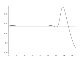
(a) Charge $q(r)$

(b) Statistics parameter ${\nu}(r)$

Figure 14: (a): The charge $q(r)$ as a function of the quasi-electron’s distance from the origin. (b): The statistics parameter ${\nu}(r)$ as a function of half the distance between the quasi-electrons. The system has 74 electrons, and for comparison we have included the horizontal lines $1/3$ and $-1/3$.

Notice that even for $r\rightarrow 0$, $q$ stays close to the plateau rather than dropping to zero as does the integrated single-electron density; compare to Fig. 10. This emphasizes that the present definition of the charge does not necessarily give the same charge as the one found by integrating the single-electron density. When we interpret the Berry phase as an Aharonov-Bohm phase, the behaviour as $r\rightarrow 0$ can in the present case be understood in the following way: The Aharonov-Bohm phase $\gamma$ associated with the loop $z_{0}=re^{i\phi}$ is proportional to the encircled magnetic flux. The curve in Fig. 14a shows $\frac{1}{2\pi r^{2}}\gamma$, which then is a constant. This holds even if the charge is not truly point like, because all parts of the smeared out charge is moved around in equal loops.

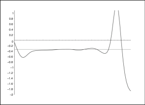
(a) Statistics parameter for Jain quasi-electrons.

(b) Statistics parameter for Laughlin quasi-electrons.

Figure 15: Comparison between curves that define the statistics parameters of (a): Jain quasi-electrons (80), and (b): Laughlin quasi-electrons. For the Jain quasi-electrons we have used a system with 74 electrons, whereas the Laughlin quasi-electron curves are for systems with 20, 50, 75, 100 and 200 electrons. Of these the 75 electron curve is farthest to the right, and the figure is from Ref. [6].

We now turn to Fig. 14b where the statistics parameter ${\nu}(r)$, as given by Eq. (80), is shown as a function of $r$. The figure shows that there is a range of $r$ for which the value of $\nu$ is approximately constant. That is, we see rather clear signs of a well defined bulk value for the statistics parameter of the Jain quasi-electrons. To give unquestionable evidence for the existence of such a plateau, and also to determine the precise value of the parameter, would require more detailed studies than we have done here. However, we do observe that the value $-1/3$ seems likely to be the value of the statistics parameter $\nu$. This equals minus the statistics parameter of the Laughlin quasi-holes. Let us mention that we also for a system with 50 electrons have seen clear indications of this.

The results seen here for the Jain quasi-electrons are similar to the results obtained in Ref. [6] for the Laughlin quasi-hole. But the most striking observation is the big difference between the results found in this reference for the Laughlin quasi-electron, and the present results for the Jain quasi-electron. Fig. 15 shows a comparison between the curves that are used to define the statistics parameter, as found from Berry phases, for these two definitions of the quasi-electron wave function, with Jain’s definition used in figure (a) and Laughlin’s definition used in (b). The latter figure is from Ref. [6], and shows results for the system sizes 20, 50, 75, 100 and 200 electrons. The 75 electron curve, which is most appropriate for comparison with our Jain quasi-electron curve for 74 electrons, is the one farthest to the right. The difference between Figs.15a and 15b is striking; whereas the curves for Laughlin quasi-electron do not show signs of a well-defined statistics parameter, that is clearly the case for the Jain quasi-electron.

The signs of the statistics parameters of the quasi-electrons deserve special attention. We note that they are different for Jain’s and Laughlin’s wave functions. Let us re-express the results in terms of the parameter $\nu_{1}$ which measures the repulsion or attraction between the quasi-particles. For the quasi-hole the value is $\nu_{1}=+1/3$, which corresponds to an effective repulsion between two quasi-holes. Compared to the quasi-hole the Jain quasi-electron has the opposite sign for the charge as well as for the statistics parameter $\nu$ [6]. This means that $\nu_{1}$ is positive also for the Jain quasi-electrons. The opposite sign for the statistics parameter, as may be indicated by the Berry phase calculations for the Laughlin quasi-electron, would correspond to an effective attraction between the quasi-electrons. In the anyon representation this attraction would be represented by a singular anyon wave function [6].

A simple picture of the quasi-particles represented as charge-flux composites indicates that (the non-integer part of) the statistics parameter $\nu_{1}$ should have opposite sign for the quasi-hole and the quasi-electron. This is because the sign of both the flux and the charge is reversed for the quasi-electron compared to the quasi-hole. This gives the same value for the parameter $\nu$, but the opposite sign for $\nu_{1}$, due to the different signs of the charges. This simple argument is supported by numerical studies of the quantum Hall effect on a sphere [23]. State counting gives an exclusion statistics parameter for the quasi-electrons which corresponds to $\nu_{1}=2-1/3$, as compared to $\nu_{1}=+1/3$ for the quasi-holes. The fractional part is negative, but it is compensated by a positive integer part to give altogether a repulsive parameter. It is of interest to note that the results obtained for Berry phase calculations of the statistics parameter do not fit this expected value of the physical quasi-electron, neither with Jain’s nor Laughlin’s wave functions for the quasi-electron.

6 Conclusions

To summarize, we have examined expectation values and fluctuations for the charge of quasi-holes and quasi-electrons in the quantum Hall system with filling fraction $1/3$. The study has been motivated by the asymmetry between quasi-holes and quasi-electrons that has previously been found in Berry phase calculations of the statistics parameter [6]. We have in particular been interested in examining to what extent the quasi-electron charge can be regarded as a sharply defined quantum number. To study these problems we have calculated charge fluctuations, as well as charge expectation values, measured relative to the ground state. We have done computations for a Laughlin quasi-hole, and for quasi-electrons both with Laughlin’s and Jain’s definition of the wave function. In all cases the quasi-particle has been located at the center of a circular electron droplet.

For the quasi-hole charge we have found numerical results that are consistent with the expected bulk value $-1/3$ (times the electron charge) and charge fluctuations consistent with vanishing fluctuations in the bulk. There are effects due to the finite size of the quasi-hole and to the finite size of the droplet, but in an intermediate interval the deviations from the expected values vanish within small statistical errors. The computations have been done for systems with 50 and 100 electrons, and the results clearly confirm the conclusion that the quasi-hole charge is a sharp quantum number.

For the Laughlin quasi-electron the calculations similarly reproduce the expected bulk value of the charge, which is $1/3$ times the electron charge. But for the charge fluctuations of this excitation we find fluctuations which survive throughout the whole electron droplet. At an absolute scale the values are small, but we have shown that they are significantly different from zero. We have studied systems with 50, 100 and 200 electrons, and conclude that results obtained for these system sizes do not unambiguously confirm the charge of the Laughlin quasi-electron to be a sharp quantum number. The deviation from zero which are found for the charge fluctuations may be a finite-size effect, but the fluctuations then are sufficiently long range that even a system of $200$ electrons is not sufficiently large to see this clearly.

For a system with 50 electrons we have also studied the charge and charge fluctuations of a Jain quasi-electron. In this case we again reproduce expected results in the bulk, $1/3$ for the charge and vanishing fluctuations. There are small deviations, but these are not significant, within small statistical errors. We also find that in this context there is almost no difference between the results obtained for the Jain wave function projected onto the lowest Landau level and the unprojected state. This confirms results presented elsewhere in the literature, which show that the unprojected state is almost entirely in the lowest Landau level.

As a further examination of the relation between sharpness of the charge and a well defined statistics parameter, we have computed Berry phases for the Jain quasi-electron. This gives a supplement to the previously done calculations for the Laughlin quasi-electron [5]. We have considered unprojected states for a system with 50 electrons, and have extracted charge and statistics parameters in the usual way. The charge parameter calculated in this way has a well defined bulk value with only a small deviation from the expected value $1/3$. The small deviation may be due the definition used for the wave function of a quasi-electron translated to arbitrary position, but we have no firm conclusion about this.

As the most interesting result of the Berry calculations, we found that the statistics parameter of the Jain quasi-electron is much more well behaved than the analogous quantity for the Laughlin quasi-electron. With the convention used here, our results clearly indicate that the value of this parameter (for large separations of the two quasi-electrons) is $\nu=-1/3$, which is minus the statistics parameter of the quasi-holes. However, the sign of the statistics parameter does not agree with the expected one, and is not consistent with the value $-2+1/3$ indicated by state counting of numerically determined energy levels for quantum Hall states on a sphere. Thus, for neither of the suggested wave functions, due to Laughlin and Jain, the expected statistics parameter of the physical quasi-electrons seem to be correctly reproduced.

Appendix A Numerical techniques

This appendix reviews important aspects of the Metropolis algorithm and Monte Carlo estimate.

In section 3 we give several examples of functions used to generate electron configurations according to the Metropolis algorithm, e.g. Eq. (15). We will briefly review the technical details of this method. Suppose then that the desired (real) probability distribution is given by $p(z_{1},\cdots,z_{N}^{*})$, and there is a given configuration $\{z_{i,\alpha}\}_{i=1}^{N}$. To find the next configuration we loop through the electrons, and for each $i$ we randomly choose a test coordinate $z_{i}^{\rm t}=z_{i,\alpha}+\Delta z_{i}$ such that $\Delta z_{i}$ and $-\Delta z_{i}$ are equally probable. We then compute the ratio

$$f_{i}=\frac{p(z_{1,\alpha},\cdots,z_{i}^{\rm t},\cdots,z_{i}^{*\rm t},\cdots z_{N,\alpha}^{*})}{p(z_{1,\alpha},\cdots,z_{i\alpha},\cdots,z_{i\alpha}^{*},\cdots z_{N,\alpha}^{*})}$$ (83)

If the number $f_{i}$ is larger than a randomly generated number between $0$ and $1$, then we accept the test coordinate and set $z_{i,\alpha+1}=z_{i}^{\rm t}$. Otherwise $z_{i,\alpha+1}=z_{i,\alpha}$. The procedure ensures that the configurations are generated according to the desired probability distribution $p$ because the principle of detailed balance is satisfied by the transition probabilities; the ratio of jumping from $z_{a}$ to $z_{b}$ or from $z_{b}$ to $z_{a}$ equals the ratio $p(z_{b})/p(z_{a})$.

For the cases we have considered it is of special interest to notice that an overall normalization factor in $p$ is irrelevant for the Metropolis algorithm since the latter only considers ratios between different value of $p$. In all our calculations of charge and charge fluctuations we have benefited from this in the sense that we have used probability distributions for which we did not know how to analytically find the normalization factor. For instance the factor $I_{0}$ in Eq. (15) is not known exactly. It was essential that we could do this, because the computer time needed to obtain well converged results highly depends on the choice of probability distribution. The time is reduced when $p$ has a behaviour similar to the actual integrand of the problem under consideration, because the standard deviation of the Monte Carlo estimate is given by $\sqrt{V(g/p)/n}$, with $g$ as the specific integrand, $V(g/p)$ as the variance of the function $g/p$, and $n$ the number of Monte Carlo steps.

Appendix B Relations between ${\widetilde{Q}}(R)$, ${\widetilde{F}}(R_{1},R_{2})$ and $Q_{\rm Le}(R)$, $F_{\rm Le}(R)$

In this appendix we will show how to derive the expressions in Eqs. (36, 37).

We start by considering the relation between ${\widetilde{Q}}(R)$ and $Q_{\rm Le}(R)$. According to Eq. (22) the desired charge expectation value can be written

$$Q_{\rm Le}(R) = \frac{N}{I_{\rm Le}}\int_{A}{\rm d}^{2}\!z_{1}\int{\rm d}^{2(N-1)}\!z\,|\psi_{\rm Le}(z_{1},\cdots,z_{N}^{*})|^{2}$$ (84)

$$= 2\pi\int_{0}^{R}{\rm d}r\,rh(r),$$ (85)

where we have defined

$$h(r)=\frac{1}{2\pi}\int_{0}^{2\pi}{\rm d}\varphi\rho(z_{1},z_{1}^{*});\;\;\;\;\;\;\;z_{1}=re^{i\varphi},$$ (86)

with

$$\rho(z_{1},z_{1}^{*}) = N\frac{1}{I_{\rm Le}}e^{-|z_{1}|^{2}}\partial_{z_{1}}\partial_{z_{1}^{*}}$$ (88)

$$\int{\rm d}^{2}z_{2}\cdots{\rm d}^{2}z_{N}e^{-\sum_{i=2}^{N}|z_{i}|^{2}}\prod_{k=2}^{N}(|z_{k}|^{2}-1)\prod_{i<j}|z_{i}-z_{j}|^{2m}.$$

It is important to notice the ranges of the counting variables in this expression, which is obtained using integration by parts for all coordinates that are integrated over the entire complex plane. The function $\rho(z_{1},z_{1}^{*})$ is the exact single-electron density. We now define the quantities

$${\tilde{\rho}}(z_{1},z_{1}^{*})=N\frac{1}{I_{\rm Le}}\int{\rm d}^{2}z_{2}\cdots{\rm d}^{2}z_{N}e^{-\sum_{i=1}^{N}|z_{i}|^{2}}\prod_{k=1}^{N}(|z_{k}|^{2}-1)\prod_{i<j}|z_{i}-z_{j}|^{2m},$$ (89)

$${\tilde{h}}(r)=\frac{1}{2\pi}\int_{0}^{2\pi}{\rm d}\varphi{\tilde{\rho}}(z_{1},z_{1}^{*})$$ (90)

and

$${\widetilde{Q}}_{\rm Le}(R)=2\pi\int_{0}^{R}{\rm d}r\,r{\tilde{h}}(r).$$ (91)

The latter quantity is identical to the one defined in Eq. (34). Comparing Eqs. (88) and (89) we observe that the relation between $\rho$ and $\tilde{\rho}$ can be written

$$\rho(z_{1},z_{1}^{*})=e^{-|z_{1}|^{2}}\partial_{z_{1}}\partial_{z_{1}^{*}}\left(e^{|z_{1}|^{2}}\frac{1}{(|z_{1}|^{2}-1)}{\tilde{\rho}}(z_{1},z_{1}^{*})\right).$$ (92)

It is then straight forward to show that the radial functions $h$ and $\tilde{h}$ are related by

$$h(r)={\tilde{h}}(r)+\frac{1}{r}\frac{\rm d}{{\rm d}r}\left(\frac{r^{2}}{r^{2}-1}{\tilde{h}}(r)+\frac{1}{4}r\frac{\rm d}{{\rm d}r}\left(\frac{{\tilde{h}}(r)}{r^{2}-1}\right)\right).$$ (93)

This implies that

$$Q_{\rm Le}(R) = 2\pi\int_{0}^{R}{\rm d}r\,rh(r)$$ (94)

$$= 2\pi\int_{0}^{R}{\rm d}r\,r{\tilde{h}}(r)+2\pi\left(\frac{R^{2}}{R^{2}-1}{\tilde{h}}(R)+\frac{1}{4}R\left(\frac{\rm d}{{\rm d}r}\frac{{\tilde{h}}(r)}{(r^{2}-1)}\right)_{r=R}\right),$$ (95)

since the contribution from $r=0$ is zero. Notice that the appearant singularity at $r=1$ is artificial since the factor $r^{2}-1$ in the denominators is canceled by the same factor in the numerators; recall the definition of ${\tilde{h}}(r)$. Using the fact that

$$2\pi{\tilde{h}}(R)=\frac{1}{R}\frac{{\rm d}{\widetilde{Q}}(R)}{{\rm d}R}$$ (96)

we finally obtain the advertised relation

$$Q_{\rm Le}(R)={\widetilde{Q}}(R)+c_{1}(R)\frac{{\rm d}{\widetilde{Q}}(R)}{{\rm d}R}+c_{2}(R)\frac{{\rm d}^{2}{\widetilde{Q}}(R)}{{\rm d}R^{2}},$$ (97)

with

$$c_{1}(R)=\frac{4R^{4}-7R^{2}+1}{4R(R^{2}-1)^{2}}, c_{2}(R)=\frac{1}{4(R^{2}-1)}.$$ (98)

To find the relation between $F_{\rm Le}(R)$ and ${\widetilde{F}}(R_{1},R_{2})$ we perform a calculation that is similar in spirit, although technically more complicated than the one above. First we define the radial function

$$h_{2}(r_{1},r_{2})=\frac{1}{4\pi^{2}}\int_{0}^{2\pi}{\rm d}\varphi_{1}{\rm d}\varphi_{2}\rho_{2}(z_{1},z_{2},z_{1}^{*},z_{2}^{*});\;\;\;\;\;\;\;z_{1}=re^{i\varphi_{1}},z_{2}=re^{i\varphi_{2}},$$ (99)

with

$$\rho_{2}(z_{1},z_{2},z_{1}^{*},z_{2}^{*}) = N(N-1)\frac{1}{I_{\rm Le}}e^{-|z_{1}|^{2}-|z_{2}|^{2}}\partial_{z_{1}}\partial_{z_{1}^{*}}\partial_{z_{2}}\partial_{z_{2}^{*}}$$ (101)

$$\times\int{\rm d}^{2}z_{3}\cdots{\rm d}^{2}z_{N}e^{-\sum_{i=3}^{N}|z_{i}|^{2}}\prod_{k=3}^{N}(|z_{k}|^{2}-1)\prod_{i<j}|z_{i}-z_{j}|^{2m}$$

as the true two-particle distribution function. We can then write the desired function in Eq. (29) as

$$F_{\rm Le}(R)=4\pi^{2}\int_{0}^{R}{\rm d}r_{1}\,\int_{0}^{R}{\rm d}r_{2}\,r_{1}r_{2}h_{2}(r_{1},r_{2}).$$ (102)

Let us now define the auxiliary quantities

$${\tilde{\rho}}_{2}(z_{1},z_{2},z_{1}^{*},z_{2}^{*}) = N(N-1)\frac{1}{I_{\rm Le}}$$ (104)

$$\times\int{\rm d}^{2}z_{3}\cdots{\rm d}^{2}z_{N}e^{-\sum_{i=1}^{N}|z_{i}|^{2}}\prod_{k=1}^{N}(|z_{k}|^{2}-1)\prod_{i<j}|z_{i}-z_{j}|^{2m},$$

$${\tilde{h}}_{2}(r_{1},r_{2})=\frac{1}{4\pi^{2}}\int_{0}^{2\pi}{\rm d}\varphi_{1}{\rm d}\varphi_{2}{\tilde{\rho}}_{2}(z_{1},z_{2},z_{1}^{*},z_{2}^{*}),$$ (105)

and

$${\widetilde{F}}(R_{1},R_{2})=4\pi^{2}\int_{0}^{R_{1}}{\rm d}r_{1}\,r_{1}\int_{0}^{R_{2}}{\rm d}r_{2}\,r_{2}{\tilde{h}}_{2}(r_{1},r_{2}).$$ (106)

Analogous to what we saw above, also now the relation between the two-electron density $\rho_{2}$ and the quantity ${\tilde{\rho}}_{2}$ is easily established, and it reads

$$\rho_{2}=e^{-|z_{1}|^{2}-|z_{2}|^{2}}\partial_{z_{1}}\partial_{z_{1}^{*}}\partial_{z_{2}}\partial_{z_{2}^{*}}\left(\frac{e^{|z_{1}|^{2}+|z_{2}|^{2}}}{(|z_{1}|^{2}-1)(|z_{2}|^{2}-1)}{\tilde{\rho}}_{2}\right).$$ (107)

A similar exact relation exists between the radial quantities $h_{2}(r_{1},r_{2})$ and ${\tilde{h}}_{2}(r_{1},r_{2})$. We rewrite it into a form suited for integration and find

$$h_{2}(r_{1},r_{2}) = {\tilde{h}}_{2}(r_{1},r_{2})$$ (108)

$$+(r_{2}^{2}-1)\frac{1}{r_{1}}\frac{\partial}{\partial r_{1}}\left(r_{1}^{2}g_{2}\right)+(r_{1}^{2}-1)\frac{1}{r_{2}}\frac{\partial}{\partial r_{2}}\left(r_{2}^{2}g_{2}\right)$$

$$+\frac{1}{4}(r_{2}^{2}-1)\frac{1}{r_{1}}\frac{\partial}{\partial r_{1}}\left(r_{1}\frac{\partial g_{2}}{\partial r_{1}}\right)+\frac{1}{4}(r_{1}^{2}-1)\frac{1}{r_{2}}\frac{\partial}{\partial r_{2}}\left(r_{2}\frac{\partial g_{2}}{\partial r_{2}}\right)$$

$$+\frac{1}{4}\frac{1}{r_{1}r_{2}}\frac{\partial}{\partial r_{1}}\left(r_{1}\frac{\partial}{\partial r_{1}}\frac{\partial}{\partial r_{2}}(r_{2}^{2}g_{2})\right)+\frac{1}{4}\frac{1}{r_{1}r_{2}}\frac{\partial}{\partial r_{2}}\left(r_{2}\frac{\partial}{\partial r_{1}}\frac{\partial}{\partial r_{2}}(r_{1}^{2}g_{2})\right)$$

$$+\frac{1}{r_{1}r_{2}}\frac{\partial}{\partial r_{1}}\frac{\partial}{\partial r_{2}}(r_{1}^{2}r_{2}^{2}g_{2})$$

$$+\frac{1}{16}\frac{1}{r_{1}r_{2}}\frac{\partial}{\partial r_{1}}r_{1}\frac{\partial}{\partial r_{1}}\frac{\partial}{\partial r_{2}}r_{2}\frac{\partial}{\partial r_{2}}g_{2}.$$

We have in this expression used the notation $g_{2}(r_{1},r_{2})=\frac{1}{(r_{1}^{2}-1)(r_{2}^{2}-1)}{\tilde{h}}_{2}(r_{1},r_{2})$, and notice that $r_{1}$ and $r_{2}$ are treated symmetrically in Eq. (108). In what proceeds we will not in detail evaluate the integral of every term in this expression. That is a tedious job, and not very informative. Instead, we will show an example that is representative and hence give the idea for how to do the other calculations. So let us consider the first term in the second line of Eq. (108), and integrate it the way we need in order to find $F_{\rm Le}(R)$. This yields

$$4\pi^{2}\int_{0}^{R}{\rm d}r_{1}\,r_{1}\int_{0}^{R}{\rm d}r_{2}\,r_{2}(r_{2}^{2}-1)\frac{1}{r_{1}}\frac{\partial}{\partial r_{1}}\left(r_{1}^{2}g_{2}\right)$$ (109)

$$= 4\pi^{2}\int_{0}^{R}{\rm d}r_{2}\,r_{2}(r_{2}^{2}-1)\left[r_{1}^{2}g_{2}(r_{1},r_{2})\right]_{0}^{r_{1}=R}$$

$$= 4\pi^{2}\frac{R^{2}}{(R^{2}-1)}\int_{0}^{R}{\rm d}r_{2}\,r_{2}{\tilde{h}}_{2}(R,r_{2})$$

$$= 4\pi^{2}\frac{R}{(R^{2}-1)}\left(\frac{\partial{\widetilde{F}}(R_{1},R_{2})}{\partial R_{1}}\right)_{R_{1},R_{2}=R}.$$

The last equality sign shows the relation between $\tilde{h}$ and one of the derivatives of $\widetilde{F}$. This expression easily follows from Eq. (106). Other derivatives can be similarly expressed, and we use the relations

$$\frac{\partial^{2}{\widetilde{F}}(R_{1},R_{2})}{\partial R_{1}R_{2}}=4\pi^{2}R_{1}R_{2}{\tilde{h}}(R_{1},R_{2}),$$ (110)

$$\frac{\partial^{2}{\widetilde{F}}(R_{1},R_{2})}{\partial R_{1}^{2}}=\frac{1}{R_{1}}\frac{\partial{\widetilde{F}}(R_{1},R_{2})}{\partial R_{1}}+4\pi^{2}R_{1}\int_{0}^{R_{2}}{\rm d}r_{2}\,r_{2}\frac{\partial{\tilde{h}}(R_{1},r_{2})}{\partial R_{1}},$$ (111)

along with trivial extensions to $\frac{\partial^{3}{\widetilde{F}}(R_{1},R_{2})}{\partial R_{1}^{2}R_{2}}$ and $\frac{\partial^{4}{\widetilde{F}}(R_{1},R_{2})}{\partial R_{1}^{2}R_{2}^{2}}$. Performing the integrations of all terms in Eq. (108) and collecting together similar terms we end up with the expression in Eq. (37), that is

$$F_{\rm Le}(R) = {\widetilde{F}}(R,R)+c_{1}(R)\left(\frac{\partial{\widetilde{F}}}{\partial R_{1}}+\frac{\partial{\widetilde{F}}}{\partial R_{2}}\right)_{R}$$ (112)

$$+c_{2}(R)\left(\frac{\partial^{2}{\widetilde{F}}}{\partial R_{1}^{2}}+\frac{\partial^{2}{\widetilde{F}}}{\partial R_{2}^{2}}\right)_{R}+c_{1}^{2}(R)\left(\frac{\partial^{2}{\widetilde{F}}}{\partial R_{1}R_{2}}\right)_{R}$$

$$+c_{1}(R)c_{2}(R)\left(\frac{\partial^{3}{\widetilde{F}}}{\partial R_{1}^{2}R_{2}}+\frac{\partial^{3}{\widetilde{F}}}{\partial R_{1}R_{2}^{2}}\right)_{R}+c_{2}^{2}(R)\left(\frac{\partial^{4}{\widetilde{F}}}{\partial R_{1}^{2}R_{2}^{2}}\right)_{R}.$$

References

-
[1]
L. Saminadayer, D. C. Glattli, Y. Jin and B. Etienne,
Observation of the fractionally charged Laughlin
quasiparticles, Phys. Rev. Lett. 79 (1997)
2526.
R. de-Picciotto, M. Reznikov, M. Heiblum, V. Umansky, G. Bunin and D. Mahalu, Direct Observation of a Fractional Charge, Nature 389 (1997) 162. - [2] R. B. Laughlin, Anomalous Quantum Hall Effect: An Incompressible Quantum Fluid with Fractionally Charged Excitations, Phys. Rev. Lett. 50 (1983) 1395.
- [3] D. Arovas, J. R. Schriffer and F. Wilczek, Fractional Statistics and the Quantum Hall Effect, Phys. Rev. Lett. 53 (1984) 722.
- [4] J. K. Jain, Composite-Fermion Approach for the Fractional Quantum Hall Effect, Phys. Rev. Lett. 63 (1989) 199.
- [5] H. Kjønsberg and J. M. Leinaas, On the anyon description of the Laughlin hole states, Int. Jour. Mod. Phys. A 12 (1997) 1975.
- [6] H. Kjønsberg and J. Myrheim, Numerical study of charge and statistics of Laughlin quasi-particles, to appear in Int. Jour. Mod. Phys. A.
- [7] S. Kivelson and M. Roček, Consequences of gauge invariance for fractionally charged quasi-particles, Phys. Lett. 156B (1985) 85.
- [8] S. Kivelson and J. R. Schrieffer, Fractional charge, a sharp quantum observable, Phys. Rev. B 25 (1982) 6447.
- [9] R. Rajaraman and J. S. Bell, On solitons with half integral charge, Phys. Lett. 116B (1982) 151.
- [10] A. S. Goldhaber and S. Kivelson, Local charge versus Aharonov-Bohm charge, Phys. Lett. B 255 (1991) 445.
- [11] F. James, Monte Carlo theory and practice, Rep. Prog. Phys. 43 (1980) 1145.
- [12] R. B. Laughlin in The Quantum Hall Effect eds. R. E. Prange and S. M. Girvin, Springer-Verlag, 1990.
- [13] R. Morf and B. I. Halperin, Monte Carlo evaluation of trial wave functions for the fractional quantized Hall effect: Disk geometry, Phys. Rev. B 33 (1986) 2221.
- [14] F. D. M. Haldane and E. H. Rezayi, Finite-Size Studies of the Incompressible State of the Fractionally Quantized Hall Effect and its Excitations, Phys. Rev. Lett. 54 (1985) 237.
- [15] N. Trivedi and J. K. Jain, Numerical Study of Jastrow-Slater Trial States for the Fractional Quantum Hall Effect, Mod. Phys. Lett. B 5 (1991) 503.
- [16] S. M. Girvin and T. Jach, Formalism for the Quantum Hall Effect: Hilbert space of analytic functions, Phys. Rev. B 29 (1984) 5617.
- [17] W. H. Press, W. T. Vetterling, S. A. Teukolsky and B. P. Flannery, Numerical Recipes in C, Cambridge University Press, 1992.
- [18] M. B. Berry, Quantal phase factors accompanying adiabatic changes, Proc. R. Soc. Lond. A. 392 (1984) 45.
- [19] Y. Aharonov and D. Bohm, Significance of electromagnetic potentials in the quantum theory, Phys. Rev. 115 (1959) 485.
- [20] T. H. Hansson, J. M. Leinaas and J. Myrheim, Dimensional reduction in anyon systems, Nucl. Phys. B 384 (1992) 559.
- [21] F. D. M. Haldane, “Fractional statistics” in arbitrary dimensions: A generalization of the Pauli principle, Phys. Rev. Lett. 67 (1991) 937.
- [22] G. Dev and J.K. Jain, Jastrow-Slater trial wave functions for the fractional quantum Hall effect: Results for few-particle systems, Phys. Rev. B 45 1223 (1992).
- [23] M. D. Johnson and G. S. Canright, Haldane fractional statistics in the fractional quantum Hall effect, Phys. Rev. B 49 (1994) 2947.