Spin domains in ground state spinor Bose-Einstein condensates

J. Stenger, S. Inouye, D.M. Stamper-Kurn, H.-J. Miesner, A.P. Chikkatur, and W. Ketterle

Department of Physics and Research Laboratory of Electronics,
Massachusetts Institute of Technology, Cambridge, MA 02139

Bose–Einstein condensates of dilute atomic gases, characterized by a macroscopic population of the quantum mechanical ground state, are a new, weakly interacting quantum fluid [1, 2, 3]. In most experiments condensates in a single weak field seeking state are magnetically trapped. These condensates can be described by a scalar order parameter similar to the spinless superfluid ⁴He. Even though alkali atoms have angular momentum, the spin orientation is not a degree of freedom because spin flips lead to untrapped states and are therefore a loss process. In contrast, the recently realized optical trap for sodium condensates [4] confines atoms independently of their spin orientation. This opens the possibility to study spinor condensates which represent a system with a vector order parameter instead of a scalar. Here we report a study of the equilibrium state of spinor condensates in an optical trap. The freedom of spin orientation leads to the formation of spin domains in an external magnetic field. The structure of these domains are illustrated in spin domain diagrams. Combinations of both miscible and immiscible spin components were realized.

A variety of new phenomena is predicted [5, 6, 7] for spinor condensates, such as spin textures, propagation of spin waves and coupling between superfluid flow and atomic spin. To date such effects could only be studied in superfluid ³He, which can be described by Bose–Einstein condensation of Cooper pairs of quasi particles having both spin and orbital angular momentum [8]. Compared to the strongly interacting ³He, the properties of weakly interacting Bose–Einstein condensates of alkali gases can be calculated by mean field theories in a much more straightforward and simple way.

Other systems which go beyond the description with a single scalar order parameter are condensates of two different hyperfine states of ⁸⁷Rb confined in magnetic traps. Recent experimental studies have explored the spatial separation of the two components [9, 10] and their relative phase [11]. Several theoretical papers describe their structure [12, 13, 14, 15, 16, 17, 18] and their collective excitations [19, 20, 21, 22].

Compared to these two–component condensates, spinor condensates have several new features including the vector character of the order parameter and the changed role of spin relaxation collisions which allow for population exchange among hyperfine states without trap loss. In contrast, for ⁸⁷Rb experiments trap loss due to spin relaxation severely limits the lifetime.

We consider an $F\!=\!1$ spinor condensate subject to spin relaxation, in which two $m_{F}\!=\!0$ atoms can collide and produce an $m_{F}\!=\!+1$ and an $m_{F}\!=\!-1$ atom and vice versa. We investigate the distribution of hyperfine states and the spatial distribution in equilibrium assuming conservation of the total spin.

The ground state spinor wave function is found by minimizing the free energy [5]

$$K=\int\,d^{3}r\,n\left[V+\frac{c_{0}n}{2}+\frac{c_{2}n}{2}\langle\vec{F}\rangle^{2}+E_{ze}-p_{0}\langle F_{z}\rangle\right],$$ (1)

where kinetic energy terms are neglected in the Thomas-Fermi approximation which is valid as long as the dimension of spin domains (typically 50 $\mu m$) is larger then the penetration depth [18] (typically 1 $\mu m$). $V$ is the trapping potential, $n$ is the density, $\vec{F}$ is the angular momentum per atom, and $E_{ze}$ is the Zeeman energy in an external magnetic field. The Lagrange multiplier $p_{0}$ accounts for the total spin conservation. The mean field energy in Eqn. (1) consists of a spin independent part proportional to $c_{0}$ and a spin dependent part proportional to $c_{2}\langle\vec{F}\rangle^{2}$. The coefficients $c_{0}$ and $c_{2}$ are related to the scattering lengths $a_{0}$ and $a_{2}$ for two colliding atoms with total angular momentum $F_{tot}=0$ or $F_{tot}=2$ by $c_{0}=4\pi\hbar^{2}\bar{a}/M$ and $c_{2}=4\pi\hbar^{2}\Delta a/M$ with $\bar{a}=(2a_{2}+a_{0})/3$, $\Delta a=(a_{2}-a_{0})/3$, and $M$ for the atomic mass [5]. The spin dependent interaction originates from the term $c_{2}\vec{F_{1}}\cdot\vec{F_{2}}$ in the interaction of two atoms, which is ferromagnetic for $c_{2}<0$ and anti–ferromagnetic for $c_{2}>0$.

In the Bogoliubov approach the many–body ground state wave function is represented by the spinor wave function

$$\Psi(\vec{r})=\sqrt{n(\vec{r})}\;\zeta(\vec{r})=\sqrt{n(\vec{r})}\;\left(\zeta_{+}(\vec{r}),\zeta_{0}(\vec{r}),\zeta_{-}(\vec{r})\right),$$ (2)

where $\zeta_{+},\zeta_{0},\zeta_{-}$ denote the amplitudes for the $m_{F}\!=+1,0,-1$ states, respectively, and $|\zeta|^{2}=1$.

The Zeeman energy $E_{ze}$ is given by

$$E_{ze}=E_{+}|\zeta_{+}|^{2}+E_{0}|\zeta_{0}|^{2}+E_{-}|\zeta_{-}|^{2}=E_{0}-\tilde{p}\,\langle F_{z}\rangle+q\,\langle F_{z}^{2}\rangle.$$ (3)

$E_{+},E_{0},E_{-}$ are the Zeeman energies of the $m_{F}=+1,0,-1$ states, $2q\equiv E_{+}+E_{-}-2E_{0}$ is the Zeeman energy difference in a spinflip collision, and $2\tilde{p}\equiv E_{-}-E_{+}$. The $E_{0}$ term can be included in the trapping potential $V$. The parameter $\tilde{p}$ can be combined with the Lagrange multiplier $p_{0}$ to give $p\equiv\tilde{p}+p_{0}$.

In the following we determine the spinor which minimizes the spin–dependent part $K_{s}$ of the free energy:

$$K_{s}=c\,\langle\vec{F}\rangle^{2}-p\,\langle F_{z}\rangle+q\,\langle F_{z}^{2}\rangle,$$ (4)

where $c=c_{2}n/2$. The minimization of Eqn. (4) for different values of the parameters c, p, and q is straightforward, and is shown graphically in the form of spin-domain diagrams in Fig. 1.

Experimentally, the values of c, p, and q can be varied arbitrarily, representing any region of the spin domain diagram. The magnitude (but not the sign) of the coefficient $c$ is varied by changing the density $n$, either by changing the trapping potential, or by studying condensates with different numbers of atoms. In this study, the axial length of the trapped condensate is more than 60 times larger than its radial size, and thus we consider the system one–dimensional, and integrate over the radial coordinates, obtaining $n=2n_{0}/3$ where $n_{0}$ is the density at the radial center. This integration assumes a parabolic density profile within the Thomas–Fermi approximation. The value of $q$ can be changed by applying a weak external bias field $B_{0}$; $q$ then corresponds to the quadratic Zeeman shift $q=\hat{q}B_{0}^{2}$. The coefficient $p$ arises both from the linear Zeeman shift and from the Lagrange multiplier $p_{0}$ which is determined by the total spin of the system. For a system with zero total spin in a homogenous bias field $B_{0}$, $p_{0}$ cancels the linear Zeeman shift due to $B_{0}$, yielding $p=0$. Positive (negative) values of $p$ are achieved for condensates with a positive (negative) overall spin. Finally, the coefficients can be made to vary spatially across the condensate. In particular, applying a field gradient $B^{\prime}$ along the axis of the trapped condensate causes $p$ to vary along the condensate length. For a condensate with zero total spin, $p=\mu B^{\prime}z$ where $z$ is the axial coordinate with $z=0$ at the center of the condensate. Thus, the condensate samples a vertical line in the spin domain diagrams of Fig. 1. The center of this line lies at $p=0$, and its length is given by the condensate length scaled by $\mu B^{\prime}$.

The experimental study of spinor condensates required techniques to selectively prepare and probe condensates in arbitrary hyperfine states. Spinor condensates were prepared in several steps. Laser cooling and evaporative cooling were used to produce sodium condensates in the $m_{F}\!=\!-1$ state in a cloverleaf magnetic trap [23]. The condensates were then transfered into an optical dipole trap consisting of a single focused infrared laser beam [4]. Arbitrary populations of the three hyperfine states were prepared using rf transitions [4]. After the spin preparation, a bias field $B_{0}$ and a field gradient $B^{\prime}$ were applied for a variable amount of time (as long as 30 s), during which the atoms relaxed towards their equilibrium distribution, as shown in fig. 2.

The profiles in Fig. 3 were obtained from vertical cuts through absorption images. They provide clear evidence of anti–ferromagnetic interaction. The spin structure is consistent with the corresponding spin domain diagram in fig. 1 a. Overlapping $m_{F}\!=\!\pm 1$ clouds as observed are incompatible with the assumption of ferromagnetic interaction.

The strength $c=(50\pm 20)\,{\rm Hz}$ of the anti–ferromagnetic interaction was estimated by determining $z_{b}$, the location of the $m_{F}\!=\!0$ to the $m_{F}\!=\!\pm 1$ boundary, and by plotting $p=\mu B^{\prime}z_{b}$ versus the quadratic Zeeman shift $q=\hat{q}B_{0}^{2}$ as shown in Fig. 4. With $n=(2.9\pm 0.5)\times 10^{14}\,{\rm cm}^{-3}$ the difference between the scattering lengths can be determined to $a_{2}-a_{0}=3\Delta a=(3.5\pm 1.5)a_{B}=(0.19\pm 0.08)\,{\rm nm}$ where $a_{B}$ denotes the Bohr radius. This result is in rough agreement with a theoretical calculation of $a_{2}-a_{0}=(5.5\pm 0.5)a_{B}$ [24]. The anti–ferromagnetic interaction energy corresponds to 2.5 nK in our condensates. Still, the magnetostatic (ferromagnetic) interaction between the atomic magnetic moments is about ten times weaker. It is interesting to note that the optically trapped samples in which the domains were observed were at a temperature of the order of 100 nK, far larger than the anti–ferromagnetic energy. The formation of spin domains occurs only in a Bose–Einstein condensate.

Fig. 3 c shows a profile of the density distribution for a cloud at $B_{0}=20\,{\rm mG}$ and almost canceled gradient ($B^{\prime}<2\,{\rm mG/cm}$). No $m_{F}=0$ region can be identified. The cloud was prepared with a small total angular momentum. Due to the almost–zero gradient and the non–zero angular momentum the cloud corresponds to a point in the shaded region in Fig. 1 a, rather than a vertical line with no offset as discussed before with finite gradients and zero angular momentum. The different widths of the profiles are probably caused by residual field inhomogenities. Fig. 3 c demonstrates the complete miscibility of the $m_{F}=\pm 1$ components.

For a homogenous two–component system the criterion for miscibility (immiscibility) is $a_{ab}<(>)\sqrt{a_{a}a_{b}}$ [14, 15, 18], when the mean field energy is parametrized as $(2\pi\hbar^{2}/M)(n_{a}^{2}a_{a}+n_{b}^{2}a_{b}+2n_{a}n_{b}a_{ab})$. Here, $n_{a,b}$ and $a_{a,b}$ are densities and scattering lengths for the components $a$ and $b$, and the scattering length $a_{ab}$ characterizes the interactions between particles $a$ and $b$. In our spinor condensate with mixtures of the $m_{F}\pm 1$ components, we have $a_{-1}=a_{+1}=\bar{a}+\Delta a$ and $a_{-1\,+1}=\bar{a}-\Delta a$. Thus $\Delta a>0$, like experimentally observed, implies miscibility. For a mixture of the $m_{F}=1$ and $m_{F}=0$ components, we find $a_{0}=\bar{a},\quad a_{+1}=\bar{a}+\Delta a$ and $a_{0\,+1}=\bar{a}+\Delta a$, corresponding to immiscibility. For the ⁸⁷Rb experiments [9, 10] it is not clear whether the two components are miscible or overlap only in a surface region due to kinetic energy [25].

In conclusion, Bose–Einstein condensates of sodium occupying all three hyperfine states of the $F=1$ ground state multiplet were optically trapped in low magnetic fields. The hyperfine states are coupled by spin–exchange processes, resulting in the formation of spin domains. We developed spin domain diagrams for both the anti–ferromagnetic and the ferromagnetic case, and showed that sodium has anti–ferromagnetic interactions, whereas the opposite case is predicted for the ⁸⁷Rb $F=1$ spin multiplet [24]. All regions in the spin domain diagrams are accessible with our experimental technique and thus any combination of the three hyperfine components can be realized by applying small external magnetic fields. Of special interest for future work is the zero magnetic field case, where the rotational symmetry should be spontaneously broken. We observed both miscibility and immiscibility of hyperfine components. Thus the dynamics and possible metastable configurations [7] of two interpenetrating, miscible superfluid components ($m_{F}\!=\!\pm 1$) with arbitrary admixtures of an immiscible component ($m_{F}\!=\!0$) can now be studied.

We acknowledge stimulating discussions with Jason Ho and Chris Greene. This work was supported by the Office of Naval Research, NSF, Joint Services Electronics Program (ARO), NASA, and the David and Lucile Packard Foundation. J.S. would like to acknowledge support from the Alexander von Humboldt-Foundation, D.M.S.-K. from the JSEP Graduate Fellowship Program, and A.P.C. from the NSF.

Figure caption 1: Spin domain diagrams for spin–one condensates. The structure of the ground state spinor is shown as a function of the linear ($\sim p$) and quadratic ($\sim q$) Zeeman energies. Hyperfine components are mixed inside the shaded regions. Solid lines indicate a discontinuous change of state populations whereas dashed lines indicate a gradual change. The behaviour for $q<0$ is also shown although it is not relevant for this experiment. For $c=0$, the Zeeman energy causes the cloud to separate into three domains with $m_{F}=+1,0,-1$ and with boundaries at $|p|=q$, as shown in b. For $c_{2}\neq 0$, the mean field energy shifts the boundary region between domains and leads to regions of overlapping spin components. In the anti–ferromagnetic case (a), the $m_{F}\!=\!0$ component and the $m_{F}\!=\!\pm 1$ components are immiscible (including the kinetic energy terms in Eqn. (1) would lead to a thin boundary layer) and the boundary occurs at $|p|=q+c$. For small bias fields, with $q<c$ and $|p|<2c$, the $m_{F}\!=\!0$ domain is bordered by domains in which $m_{F}\!=\!\pm 1$ components are mixed. The ratio of the $m_{F}\!=\!\pm 1$ populations in these regions does not depend on $q$, but is given by $|\zeta_{+}|^{2}/|\zeta_{-}|^{2}=(2c+p)/(2c-p)$. In this region of small fields, the boundary to the $m_{F}\!=\!0$ component lies at $|p|=2\sqrt{cq}$. In the ferromagnetic case (c) all three components are generally miscible, and have no sharp boundaries. Pure $m_{F}\!=\!0$ domains occur for $|p|\leq\sqrt{q(q-4|c|)}$ and pure $m_{F}\!=\!\pm 1$ domains for $|p|>q$. Here, in contrast to the anti–ferromagnetic case, a pure $m_{F}\!=\!0$ condensate is skirted by regions where it is mixed predominantly with either the $m_{F}\!=\!-1$ or the $m_{F}\!=\!+1$ component. The contribution of the third component is very small ($<2\,\%$). In all mixed regions the $m_{F}\!=\!0$ component is never the least populated of the three spin components. This qualitative feature can be used to rule out that $F=1$ sodium atoms have ferromagnetic interactions.

Figure caption 2: Formation of ground state spin domains. Absorption images of ballistically expanding spinor condensates show both the spatial and hyperfine distributions. Arbitrary populations of the three hyperfine states were prepared using rf transitions (Landau–Zener sweeps) [4]. At a bias field of about $40\,{\rm G}$ the transitions from $m_{F}\!=\!-1$ to $m_{F}\!=\!0$ and from $m_{F}\!=\!0$ to $m_{F}\!=\!+1$ differ in frequency by about $0.9\,{\rm MHz}$ due to the quadratic Zeeman shift and they could be driven separately. The images of clouds with various dwell times in the trap show the evolution to the same equilibrium for condensates prepared in either a pure $m_{F}=0$ state (upper row) or in equally populated $m_{F}=\pm 1$ states (lower row). Between $5\,{\rm s}$ to $15\,{\rm s}$ dwell time, the distribution did not significantly change, although the density decreased due to three–body recombination. The bias field during the dwell time was $B_{0}=20\,{\rm mG}$ and the field gradient was $B^{\prime}=11\,{\rm mG/cm}$. These images were taken after the optical trap was suddenly switched off and the atoms were allowed to expand. Due to the large aspect ratio (typically 60), the expansion was almost purely in the radial directions. All the mean–field energy was released after less than 1 ms, after which the atoms expanded as free particles. Thus, a magnetic field gradient, which was applied after 5 ms time–of–flight to yield a Stern–Gerlach separation of the cloud, merely translated the three spin components without affecting their shapes. In this manner, the single time–of–flight images provided both a spatial and spin–state description of the trapped cloud. Indeed, the shapes of the three clouds fit together to form a smooth total density distribution. After a total time–of–flight of 25 ms the atoms were optically pumped into the $F=2$ hyperfine state and observed using the $m_{F}\!=\!+2$ to $m_{F}\!=\!+3$ cycling transition. This technique assured the same transition strength for atoms originating from different spin states. The size of the field of view for a single spinor condensate is 1.7 mm $\times$ 2.7 mm.

Figure caption 3: Miscible and immiscible spin domains. Axial column density profiles of spinor Bose-Einstein condensates are shown, obtained from time-of-flight absorption images as in Fig. 2. The profiles of the $m_{F}\!=\!\pm 1$ components were shifted to undo the Stern-Gerlach separation. At low bias fields (Fig. 3 a), the $m_{F}\!=\!0$ component was skirted on both sides by $m_{F}\!=\!\pm 1$ components with significant $m_{F}\!=\!\mp 1$ admixtures thus demonstrating the anti–ferromagnetic interaction (also visible in Fig. 2). At higher fields (Fig. 3 b), the $m_{F}\!=\!\pm 1$ components are pushed apart further by a larger $m_{F}\!=\!0$ component and the $m_{F}\!=\!\mp 1$ admixtures vanish. They could not be resolved for quadratic Zeeman energies $q>20\,{\rm Hz}$. The anti–ferromagnetic interaction leads to immiscibility of the $m_{F}\!=\!0$ and the $m_{F}\!=\!\pm 1$ components. The kinetic energy in this boundary region, which is small compared to the total mean–field energy, is released in the axial direction. Due to this axial expansion of the cloud in the time–of–flight and due to imperfections in the imaging system including the limited pixel resolution, the $m_{F}\!=\!0$ to $m_{F}\!=\!\pm 1$ boundary is not sharp. Fig. 3 c demonstrates the complete miscibility of the $m_{F}=\pm 1$ components. The magnetic field parameters were $B_{0}=20\,{\rm mG},\,B^{\prime}=11\,{\rm mG/cm}$ in a, $B_{0}=100\,{\rm mG},\,B^{\prime}=11\,{\rm mG/cm}$ in b, and $B_{0}=20\,{\rm mG},\,B^{\prime}<2\,{\rm mG/cm}$ in c.

Figure caption 4: Estimate of the anti–ferromagnetic interaction energy $c$. Plotted is the linear Zeeman energy $p=|\mu B^{\prime}z_{b}|$ at the boundary between the $m_{F}\!=\!0$ and $m_{F}\!=\!\pm 1$ regions versus the quadratic Zeeman shift $q=\hat{q}B_{0}^{2}$. $\hat{q}=g_{s}^{2}\mu_{B}^{2}/16h^{2}\nu_{hfs}=278\,{\rm Hz/G^{2}}$, and $\mu=g_{s}\mu_{B}/4h=700\,{\rm kHz/G}$, $g_{s}$ denotes the electron g–factor, $\nu_{hfs}$ the hyperfine splitting frequency, and $\mu_{B}$ the Bohr magneton. The solid line is a fit of the function $|p|=2\sqrt{qc}$ for $q<c$ and $|p|=q+c$ for $q>c$. Extrapolating the linear part to zero bias field (dashed line) yields $c=(50\pm 20)\,{\rm Hz}$. The data points at a given bias field represent $p=\mu B^{\prime}z_{b}$ for different gradient fields $B^{\prime}$ and thus $m_{F}\!=\!0$ regions of different size. The scatter of these points is mainly due to a residual magnetic field inhomogenities, resulting in small deviations of the local gradient $B^{\prime}$. The error bar represents the relative error of all data points of 30 % in $p$ and 5 % in $q$ as estimated from the uncertainties in the magnetic field calibration. Furthermore the limited pixel resolution and contributions of the kinetic energy in the condensate to the axial expansion enhance the errors for the determination of $z_{b}$ of small $m_{F}=0$ regions.

\begin{picture}(15.0,6.0)\centerline{\hbox{\epsfbox{fig1.eps}}} \end{picture}

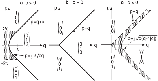
Figure 1:

\begin{picture}(15.0,10.0)\centerline{\hbox{\epsfbox{fig2.epsf}}} \end{picture}

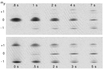
Figure 2:

\begin{picture}(10.0,9.0)\centerline{\hbox{\epsfbox{fig3.epsf}}} \end{picture}

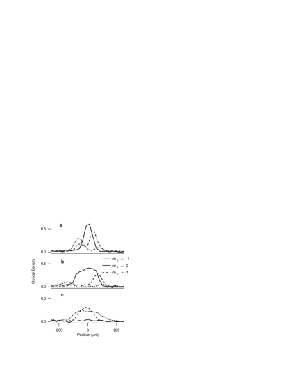
Figure 3:

\begin{picture}(10.0,7.0)\centerline{\hbox{\epsfbox{fig4.epsf}}} \end{picture}

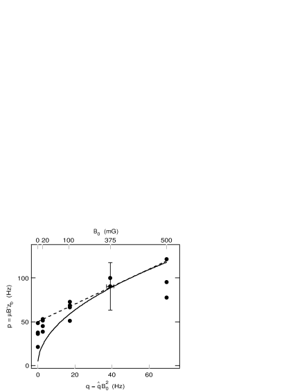
Figure 4:

References

- [1] Anderson, M. H., Ensher, J. R., Matthews, M. R., Wieman, C. E., & Cornell, E. A. Observation of Bose-Einstein condensation in a dilute atomic vapor. Science, 269, 198–201 (1995).
- [2] Davis, K. B., et al. Bose-Einstein condensation in a gas of sodium atoms. Phys. Rev. Lett., 75, 3969–3973 (1995).
- [3] Bradley, C. C., Sackett, C. A., & Hulet, R. G. Bose-Einstein condensation of lithium: Obervation of limited condensate number. Phys. Rev. Lett., 78, 985–989 (1997).
- [4] Stamper-Kurn, D. M., et al. Optical confinement of a Bose-Einstein condensate. Phys. Rev. Lett. 80, 2027–2030 (1998).
- [5] Ho, T.-L. Spinor Bose condensates in optical traps. Phys. Rev. Lett. 81, 742–745 (1998).
- [6] Ohmi, T. & Machida, K. Bose–Einstein condensation with internal degrees of freedom in alkali atom gases. J. Phys. Soc. Jpn. 67 (1998), in press.
- [7] Law, C.K., Pu, H., & Bigelow, N.P. Quantum spins mixing in spinor Bose–Einstein condensates. Phys. Rev. Lett., submitted, cond-mat/9807258 (1998).
- [8] Vollhardt, D. & Wölfle, P. The superfluid phases of 3He. Taylor–Francis, London (1990).
- [9] Myatt, C.J., Burt, E.A., Ghrist, R.W., Cornell. E.A., & Wieman, C.E. Production of two overlapping Bose–Einstein condensates by sympathetic cooling. Phys. Rev. Lett. 78, 586–589 (1997).
- [10] Hall, D.S., Matthews, M.,R., Ensher, J.R., Wieman, C.E., & Cornell, E.A. The dynamics of component separation in a binary mixture of Bose–Einstein condensates. Phys. Rev. Lett., submitted, cond-mat/9804138 (1998).
- [11] Hall, D.S., Matthews, M.,R., Wieman, C.E., & Cornell, E.A., Measurements of relative phase in binary mixtures of Bose–Einstein condensates. Phys. Rev. Lett., submitted, cond-mat/9805327 (1998).
- [12] Siggia, E.D. & Ruckenstein, A.E. Bose Condensation in spin–polarized atomic hydrogen. Phys. Rev. Lett. 44, 1423–1426 (1980).
- [13] Ho, T.-L. and Shenoy, V.B. Binary mixtures of Bose condensates of alkali atoms. Phys. Rev. Lett. 77, 3276–3279 (1996).
- [14] Timmermans, E. Phase separation in Bose–Einstein condensates. Submitted, cond-mat/9709301
- [15] Esry, B.D., Greene, C.H., Burke, J.P., and Bohn, J.L. Hartree–Fock theory for double condensates. Phys. Rev. Lett. 78, 3594–3597 (1997).
- [16] Öhberg, P. & Stenholm, S. Hartree–Fock treatment of the two–component Bose–Einstein condensate. Phys. Rev. A57, 1272–1279 (1998).
- [17] Pu, H. & Bigelow, N.P. Properties of two–species Bose condensates. Phys. Rev. Lett. 80, 1130–1133 (1998).
- [18] Ao, P. & Chui, S.T. Binary Bose–Einstein condensate mixtures in weakly and strongly segregated phases. Submitted, (1998).
- [19] Busch, T., Cirac, J.I., Pérez–García, V.M., & Zoller, P. Stability and collective excitations of a two–component Bose–Einstein condensed gas: a moment approach. Phys. Rev. A56, 2978–2983 (1997).
- [20] Graham, R. & Walls, D. Collecitve excitations of trapped binary mixtures of Bose–Einstein condensed gases. Phys. Rev. A57, 484–487 (1998).
- [21] Pu, H. and Bigelow,N.P. Collective excitations, metastability, and nonlinear response of a trapped two–species Bose–Einstein condensate. Phys. Rev. Lett. 80, 1134–1137 (1998).
- [22] Esry, B.D. & Greene, C.H. Low–lying excitations of double Bose–Einstein condensates. Phys. Rev. A57, 1265–1271 (1998).
- [23] Mewes, M.-O., et al. Bose-Einstein condensation in a tightly confining dc magnetic trap. Phys. Rev. Lett. 77, 416–419, (1996).
- [24] Burke, J.P., Greene, C.H., & Bohn, J.L. Multichannel cold collisions: simple dependencies on energy and magnetic field. Phys. Rev. Lett., submitted.
- [25] Cornell, E.A. private communication.