Study of a generalized Metropolis decision rule in auxiliary field quantum Monte Carlo

Abstract

We consider a generalization of the standard Metropolis algorithm acceptance/rejection decision rule and numerically explore its properties using auxiliary field quantum Monte Carlo. The generalization involves a free parameter which, given a criterion for proposing attempted moves, can be used to tune the average acceptance rate in a particular way. Such tuning can also potentially change Monte Carlo autocorrelation times, and the combination of the changing acceptance rate and autocorrelation times raises the possibility of more efficient simulations. We explore these issues using primarily massively parallel quantum Monte Carlo runs of the “test case” two-dimensional Hubbard model, and discuss results and applications.

I Introduction

Since its introduction[4], the “Metropolis algorithm” for Monte Carlo has become a widely used and powerful numerical tool, both for classical and quantum systems. The algorithm describes a Markov chain through states of the system with rules for first proposing a new state and then deciding whether or not to accept a move to the proposed state. In statistical mechanics simulations, the Metropolis rules by construction sample states according to their Boltzmann weights, allowing computation of expectation values. However, this Boltzmann weight sampling can be satisfied by other ways of making the acceptance/rejection decision besides the conventional one. We consider here a class of such alternative acceptance/rejection decisions and explore whether they might be used to increase simulation efficiency. We focus in this paper on auxiliary-field fermion quantum Monte Carlo simulations[5, 6, 7, 8, 9, 10, 11, 12, 13] though our approach and results may have more general application, particularly in other electron quantum Monte Carlo methods [14, 15, 16, 17, 18, 19]. We use primarily massively parallel machines in the quantum Monte Carlo simulations, which has allowed us to more easily gather data than would otherwise be possible.

One way to increase general Monte Carlo efficiency is to minimize the autocorrelation times $\tau_{e}$. $\tau_{e}$ is qualitatively defined for an observable as the number of Monte Carlo steps over which measurements of that observable remain correlated once the system has equilibrated (i.e., once the system has become independent of the initial configuration). $N$ Monte Carlo steps then correspond to approximately $N_{\rm ind}=N/\tau_{e}$ independent measurements. A particular statistical error will require a given number $N_{\rm ind}$ of uncorrelated data points. Hence, $N=N_{\rm ind}\,\tau_{e}$ steps will be required for a given desired statistical error, with reducing $\tau_{e}$ commensurately reducing Monte Carlo run time. A related consideration involves the “warm-up” or equilibration time $\tau_{w}$, a measure of the average number of steps required to go from typically low-weight initial configurations to the high-weight region of the phase space where measurements can then be taken.

In auxiliary field and other determinantal quantum Monte Carlo methods, however, another factor is introduced with regards to efficiency: an accepted move is often so much more computationally intensive than a rejected move that the time required for rejected moves can be neglected compared to the computationally dominating acceptance calculations [5, 6, 7, 8, 9, 10, 11, 20]. Then, the dominant computational time required for a simulation of $N$ steps is proportional rather to $NA_{e}=N_{\rm ind}A_{e}\tau_{e}$, where $A_{e}$ is the average equilibrated move acceptance rate, so that one now wishes to minimize the quantity $A_{e}\tau_{e}$. Analogously, the dominant required computational time for equilibration will be $A_{w}\tau_{w}$, where $A_{w}$ is an acceptance rate averaged during the warm-up process. Exploring the above efficiency issues is a major focus of the paper. One aspect of this involves the calculation of equilibration and autocorrelation times for the “test case” two-dimensional Hubbard model, which results, to the best of our knowledge, have not previously appeared.

After the introduction, we discuss various Monte Carlo algorithmic considerations, including parallelization issues, a generalization of the conventional Metropolis acceptance/rejection rule, and relevance to auxiliary field and other determinantal quantum Monte Carlo. We then explore properties of the new Metropolis generalization using primarily massively parallel auxiliary field quantum Monte Carlo simulations of the two-dimensional Hubbard model. Lastly, we discuss the numerical results and summarize.

II Monte Carlo Algorithm Considerations

A Parallelization Issues

Currently, the fastest computers available are those with a massively parallel architecture. These computers consist of hundreds to thousands of individual processors linked so that they can communicate with each other. Efficient use of these machines is governed by keeping communication time sufficiently low that computational speed scales roughly linearly with the number of processors.

One approach for using such computers in Monte Carlo simulations is to distribute a single Monte Carlo “walk” over all the processors. This allows the computational work of each step in the walk to be spread out over all the processors, but it can require a high degree of communication. This approach can be feasible for classical simulations of large systems with short-range forces, with each processor “owning” part of the system. However, it has not been shown to be efficient for determinantal quantum Monte Carlo simulations of the type we will discuss, and in particular might be expected to be less efficient for two dimensional systems.

A second approach is to let every processor perform its own independent Monte Carlo “walk”. Each processor then starts with a different initial configuration and can proceed independently of the other processors, and no communication is required until the final accumulation of results [21, 22, 23].

A potential drawback to this second approach, however, is that each processor must independently move from its typically low-weight initial configuration to the high-weight region of the phase space (“equilibration”) before measurements can start to be taken [22, 23]. Hence, while the measurement process is itself parallel, with measurements from the different processors combining to reduce statistical error, equilibration is serial. More specifically, let $N_{\rm ind}$ denote the number of independent measurements required for a desired statistical error, let $\tau_{w}$ denote the number of Monte Carlo steps required for equilibration (“warm-up”), let $\tau_{e}$ denote autocorrelation time in Monte Carlo steps, and let $N_{P}$ denote the number of processors in a parallel machine. Then, for a serial or vector machine, the required number of Monte Carlo steps $N$ is given by

$$N=\tau_{w}+N_{\rm ind}\tau_{e}.$$ (1)

Assuming a fluctuation-dissipation-type scenario, so that $\tau_{w}$ and $\tau_{e}$ have similar values, equilibration then plays a small role in the required computational time [24]. However, for a parallel machine, the number of steps required is

$$N=\tau_{w}+N_{\rm ind}\tau_{e}/{N_{P}}.$$ (2)

Hence, for a massively parallel machine with thousands of processors, equilibration provides a potential bottleneck, which could be improved by reducing $\tau_{w}$. It seems that such a bottleneck may actually be alleviated somewhat by the “sign problem”, which can necessitate a very large value of $N_{\rm ind}$ for reasonable statistical error.

B Metropolis, Symmetric, and “Generalized” Decision Rules

In Monte Carlo simulations, new moves are proposed according to some procedure and a decision is then made whether to accept the proposed move or to reject the move and remain in the current state. The proposal and decision together usually satisfy “microscopic reversibility”, or “detailed balance”[25]. The most commonly used proposal procedure stipulates that the probability of proposing a move to state $j$ given that one is currently in state $i$ is identical to the probability of proposing a move to state $i$ given that one is in state $j$, though other procedures have also been used[26, 27]. Although our analysis could be generalized, we will assume the above “symmetric” move proposal procedure throughout this paper in the case of detailed balance.

Probably the most common rule for deciding whether or not to accept a proposed move is the “Metropolis decision”. Let the Monte Carlo sampling be over the Boltzmann distribution, let $E$ denote the energy of the current state, let $E^{\prime}$ denote the energy of the proposed state, let $\Delta E=E^{\prime}-E$, and let $\beta=1/(k_{\rm B}T)$, where $T$ is the temperature and $k_{B}$ is Boltzmann’s constant. Then, as in the original Metropolis paper[4], the probability $P$ of accepting the proposed state is given by

$$P_{M}=\left\{\begin{array}[]{cc}e^{-\beta\Delta E}&,\,\Delta E>0\\ 1&,\,\Delta E\leq 0\,.\end{array}\right.$$ (3)

Another decision rule which has also been used is the so-called “symmetric rule”[28, 29],

$$P_{S}=\frac{e^{-\beta\Delta E}}{1+e^{-\beta\Delta E}}\,.$$ (4)

We note that, since $P_{M}\geq P_{S}$ for all $\beta\Delta E$, $P_{M}$ will give a higher average acceptance rate than $P_{S}$.

It was shown by Peskun under quite general assumptions that the Metropolis decision would lead to smaller statistical errors in the limit of very long simulations than would the symmetric decision if detailed balance were satisfied [30, 31], this result being most relevant to $\tau_{e}$. The result correlates with the higher Metropolis decision acceptance rate. When looking at the convergence of state distributions “operated on” by Monte Carlo decision rules, however, it was found that the symmetric decision rule was superior in certain cases, particularly those where a small number of states was accessible at each Monte Carlo step and where the quantity $\beta\Delta E$ was typically around magnitude 1.0 or less[32, 33]. This latter result is more directly relevant to $\tau_{w}$. Further, the Peskun analysis does not apply to certain cases of interest which can lead to the correct limiting (e.g., Boltzmann) distribution but which do not necessarily satisfy detailed balance, such as systematically moving through the lattice of a discrete system when proposing moves as opposed to randomly selecting lattice sites[31].

We explore here a generalization of the Metropolis and symmetric decisions[34],

$$P=\left\{\begin{array}[]{cc}\frac{e^{-\beta\Delta E}}{1+\Gamma e^{-\beta\Delta E}}&,\,\Delta E>0\\ \frac{e^{-\beta\Delta E}}{\Gamma+e^{-\beta\Delta E}}&,\,\Delta E\leq 0\end{array}\right.$$ (5)

where $\Gamma$ is a tunable parameter. Like the standard Metropolis and symmetric decision rules, the $P$ of Eq. 5 satisfies the condition

$$e^{-\beta E}\;P\left(E\rightarrow E^{\prime}\right)\;=\;e^{-\beta E^{\prime}}\;P\left(E^{\prime}\rightarrow E\right).$$ (6)

When $\Gamma=0$ we recover the Metropolis decision rule and when $\Gamma=1$ we recover the symmetric rule. For $0\leq\Gamma\leq 1$, $P$ smoothly interpolates between the Metropolis and symmetric limits. However, $P$ is also defined for any $\Gamma>1$.

FIG. 1.: Effect of $\Gamma$ on acceptance probability $P$ of Eq. 5

We show in Fig. 1 a plot of the $P$ of Eq. 5 versus $\beta\Delta E$ for different values of $\Gamma$. $P$ becomes independent of $\Gamma$ for sufficiently large magnitudes of $\beta\Delta E$. However, it has a strong $\Gamma$ dependence around $\beta\Delta E=0$, with a value at $\beta\Delta E=0$ of 1.0 when $\Gamma=0$ (Metropolis) and 0.0 as $\Gamma\rightarrow\infty$. Also, since $P$ is a monotonically decreasing function of $\Gamma$ for every value of $\beta\Delta E$, average equilibrated acceptance rates decrease monotonically with $\Gamma$.

Two similar generalizations which interpolate between the Metropolis and symmetric decision rules were proposed recently in the context of Monte Carlo dynamics by Mariz, Nobre, and Tsallis[35]. We note that the second of these generalizations (the so-called “geometric unification”) can also be further extended beyond the symmetric limit, reducing $P$ when $\beta\Delta E=0$ below the 0.5 symmetric value. We would expect the results which we will discuss for the $P$ of Eq. 5 to apply qualitatively to the generalizations of Ref. [35] as well.

C Auxiliary Field Quantum Monte Carlo Considerations

The previously-cited results regarding long-run statistical errors[30, 31] can be extended for the $P$ of Eq. 5 to any $\Gamma$, and would suggest that the Metropolis decision rule ($\Gamma=0$) is usually the most efficient in that context. However, as mentioned in the Introduction, there is the additional consideration for auxiliary field quantum Monte Carlo [5, 6, 7, 8, 9, 10, 11] that accepting a move is much more computationally expensive than rejecting one, with move acceptance dominating the computation. Then, for greatest efficiency, one wishes to minimize not the warm-up and equilibrated autocorrelation times $\tau_{w}$ and $\tau_{e}$ but rather the quantities $A_{w}\tau_{w}$ and $A_{e}\tau_{e}$, where $A_{w}$ is an average move acceptance rate during equilibration and $A_{e}$ is the average acceptance rate after equilibration. Even assuming that $\Gamma=0$ (Metropolis) had the smallest $\tau$’s, it is possible that an increase in $\tau_{w}$ or $\tau_{e}$ could be over-compensated by a decrease in $A_{w}$ or $A_{e}$, so that the optimal $\Gamma$ would assume some nonzero value as opposed to $\Gamma=0$.

Specifically, we will use the Blankenbecler-Scalapino-Sugar (BSS) quantum Monte Carlo algorithm [5, 6, 7] to explore the issue of optimal $\Gamma$ with the two-dimensional Hubbard model as a “test Hamiltonian”. The Hubbard model interactions are decoupled using the discrete Ising Hubbard-Stratonovich transformation introduced by Hirsch[8]. The Monte Carlo sampling is then performed on the Ising variables, with effective Boltzmann weights which depend on determinants of dense matrices resulting from the integrating out of the fermion degrees of freedom. We note that the usual Monte Carlo procedure (and the one which we will follow) is to systematically move through the “Ising lattice” when proposing moves, to which the Peskun analysis does not rigorously apply[31]. Also, the “step size” for this type of simulation is fixed, as the only possible move is a spin flip where the Ising spin changes sign. Hence, we do not consider in this paper effects of varying step size.

A potential additional factor is the cost required for numerically stabilizing the BSS algorithm [12, 13, 36], which for a given statistical error is proportional to $\tau_{w}$ and $\tau_{e}$ rather than $A_{w}\tau_{w}$ and $A_{e}\tau_{e}$. At relatively high and intermediate temperatures this cost is negligible, but it may constitute a significant fraction of the computational time at very low temperatures. In that case, one wishes rather to minimize quantities of the general form $\tau_{w}(A_{w}+\kappa)$ and $\tau_{e}(A_{e}+\kappa)$, where the $A$’s and $\kappa$ may be of comparable size. In the simulations which we describe, stabilization required a small fraction of the computational time.

III Results

A Procedure

Our goal was to explore the behavior in auxiliary field quantum Monte Carlo simulations of the optimal $\Gamma$ in the Monte Carlo decision rule of Eq. 5. This optimal $\Gamma$ was defined as that which led to the greatest simulation efficiency: i.e., lowest statistical error per computational cost. As noted previously, we estimated this efficiency by the quantities $A_{w}\tau_{w}$ during equilibration and $A_{e}\tau_{e}$ after equilibration, since for large systems and typical temperatures the leading contribution to the computational cost scales linearly with these quantities. Again, $A_{w}$ and $A_{w}$ are average acceptance rates during and after equilibration, respectively, and $\tau_{w}$ is the equilibration or “warm-up” time and $\tau_{e}$ the autocorrelation time.

Specifically, we simulated the two-dimensional Hubbard model[37], given by the Hamiltonian

  

$$H=-t\sum_{i,j;s}\left(c^{\dagger}_{i,j,s}c_{i+1,j,s}+c^{\dagger}_{i,j,s}c_{i,j+1,s}+h.c.\right)+U\sum_{i,j}(n_{i,j,\uparrow}-{1\over 2})(n_{i,j,\downarrow}-{1\over 2})-\mu\sum_{i,j,s}n_{i,j,s}.$$ (7)

  

Here $c^{\dagger}_{i,j,s}$ creates an electron of spin $s$ at site $(i,j)$ of a two-dimensional lattice, $n_{i,j,s}=c^{\dagger}_{i,j,s}c_{i,j,s}$ is the electron occupation number for spin $s$ at site $(i,j)$, and the hopping is between nearest neighbor sites. We chose hopping parameter $t=1.0$, inverse temperature $\beta t=t/(k_{B}T)=8$, Coulomb repulsions $U/t=4$ and $U/t=8$, and chemical potential $\mu/t=-1.2$ (giving an electron density per site of approximately 0.76, with $\mu=0.0$ corresponding to half filling). The imaginary time step was $\Delta\tau=0.125$, so that each Monte Carlo sweep contained 64 “imaginary time” slices. All simulations were performed on a $6\times 6$ lattice with periodic boundary conditions.

All of the $A_{w}$ and $\tau_{w}$ and most of the $A_{e}$ and $\tau_{e}$ data were obtained on the massively parallel Intel Paragon at the Sandia National Lab MPCRL, and most of the runs were on the full 1824 processors. Some of the $A_{e}$ and $\tau_{e}$ data were also obtained using the CRAY T90 at the SDSC.

To obtain $A_{w}$ and $\tau_{w}$ data, each utilized node of the Paragon was given a different random initial Ising configuration. The acceptance rates were then collected from each node after each sweep through the entire (space)-(imaginary time) Ising lattice. The averaging of the data from all the nodes increased the signal-to-noise ratio to the extent that fits could then be made to the decay of the acceptance rate from its initial higher value $A_{0}$, when moves are more likely due to the high probability of being in a low-weight state, to the lower equilibrated value $A_{e}$. $A_{w}$ was calculated as the average of the initial acceptance rate $A_{0}$ and the equilibrated rate $A_{e}$. Several observables $\cal O$ ($n=n_{\uparrow}+n_{\downarrow}$, $\sigma_{z}=n_{\uparrow}-n_{\downarrow}$, the staggered spin structure functions $S_{zz}(\pi,\pi)$ and $S_{xx}(\pi,\pi)$, and kinetic and total energies [9, 38]) were monitored similarly to the acceptance rate, and it was found that they all equilibrated at least as quickly as did the acceptance rate itself. Fits of the form $A_{e}+(A_{0}-A_{e})\,exp(-\tau/\tau_{w})$ were made to the acceptance rate data, defining the $\tau_{w}$’s. Typically, only data up to twenty sweeps was used in this fit, as the signal became lost in the noise for a larger number of sweeps.

A somewhat analogous procedure was followed in computing the $\tau_{e}$’s. First, for the observables $\cal O$ listed above, autocorrelation functions $C(\tau)$ were calculated from the equilibrated data using the formula

$$C(\tau)=\frac{\langle{\cal O}_{i}{\cal O}_{i+\tau}\rangle-\langle{\cal O}_{i}\rangle^{2}}{\langle{\cal O}_{i}^{2}\rangle-\langle{\cal O}_{i}\rangle^{2}},$$ (8)

where $\tau$ is the lag time. The autocorrelations were then fit to the form $exp(-\tau/\tau_{e})$, which we here took to define the equilibrated $\tau_{e}$ autocorrelation times [39]. Better statistics could be obtained for the $\tau_{e}$’s due to the existence of more equilibrated than equilibrating (warm-up) data.

Of those considered, it was found that the observable with the longest calculated autocorrelation time, $\tau_{e}$, was $n_{\uparrow}-n_{\downarrow}$. Hence, we will focus primarily on the $\tau_{e}$ behavior of $n_{\uparrow}-n_{\downarrow}$.

B Warm-Up Results

In Fig. 2 we show the equilibration of the acceptance rate during warm-up for $\Gamma=0$ (Metropolis decision) and $U/t=4$ using data averaged from 1824 processors. We also show an exponential decay fit to the relaxation of the acceptance rate from its initial to its equilibrated value.

Such fits for various values of $\Gamma$ were used to obtain the $A_{w}\tau_{w}$ results for $U/t=4$ of Fig. 3, where again $A_{w}=1/2\,(A_{0}+A_{e})$ is an average warm-up acceptance rate. (The error bars for $U/t=8$ were too large to observe statistically significant differences.) Note the drop shown in Fig. 3 in $A_{w}\tau_{w}$ when going from $\Gamma=0$ (Metropolis decision rule) to $\Gamma=1$ (“symmetric” rule), suggesting increased efficiency.

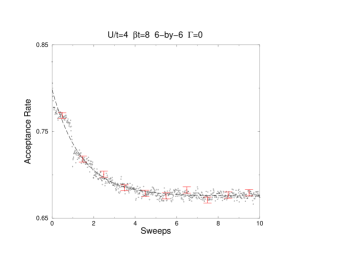
FIG. 2.: The acceptance rate for $\Gamma=0$ and $U/t=4$, shown starting from random configurations at step 0 (one sweep contains 64 imaginary time steps) until it equilibrates. For clarity, error bars are shown only once every 64 points, but all error bars are of the same general magnitude. The points are averaged data from 1824 processors. The dashed line shows a fit of the function $0.675+0.123\exp(-\tau/1.42)$

FIG. 3.: $A_{w}\tau_{w}$ versus $\Gamma$ for $U/t=4$.

C Equilibrated Results

In Fig. 4 and Fig. 5, we show data for the autocorrelation $C(\tau)$ of Eq. 8 with operator ${\cal O}=n_{\uparrow}-n_{\downarrow}$. The data were obtained by taking samples of $n_{\uparrow}-n_{\downarrow}$ at every time slice for a large number of Monte Carlo sweeps through the lattice. Also given are Monte Carlo autocorrelation times, $\tau_{e}$, obtained by an exponential fit, as well as the corresponding error bars. The $\tau_{e}$’s and errors were calculated with the use of a Fourier transform method [40]. As might be expected from the lower acceptance rates for larger $\Gamma$, the $\tau_{e}$ autocorrelation times increase for larger $\Gamma$.

FIG. 4.: Autocorrelation of $n_{\uparrow}-n_{\downarrow}$ for various values of $\Gamma$ for $U/t=4$. These curves were fit to the function $\exp(-\tau/\tau_{e})$ to obtain $\tau_{e}$.

FIG. 5.: Autocorrelation of $n_{\uparrow}-n_{\downarrow}$ for various values of $\Gamma$ for $U/t=8$. These curves were fit to the function $\exp(-\tau/\tau_{e})$ to obtain $\tau_{e}$.

As shown in Fig 6, we observed a “ringing” in the autocorrelation for the staggered spin structure function in the $z$-direction, $S_{zz}(\pi,\pi)$. No such ringing was observed for any other observable studied, including the staggered spin structure function in the $x$-direction, $S_{xx}(\pi,\pi)$. (It is known that a BSS simulation with discrete Hubbard-Stratonovich decoupling can lead to different variances for quantities with the same averages which are measured in different directions [38].)

FIG. 6.: Autocorrelation of $S_{zz}(\pi,\pi)$ for various values of $\Gamma$ for $U/t=4$. Taking just the peaks, these curves can also be fit to $\exp(-\tau/\tau_{e})$ to obtain a $\tau_{e}$ for this observable.

FIG. 7.: $A_{e}\tau_{e}$ versus $\Gamma$ for $U/t=4$ and $U/t=8$.

In Fig. 7, we show $A_{e}\tau_{e}$ for both $U/t=4$ (top) and $U/t=8$ (bottom). There were no statistically significant changes observed in $A_{e}\tau_{e}$ for $U/t=8$ in the studied range $0\leq\Gamma\leq 5$. However, for $U/t=4$, $A_{e}\tau_{e}$ was observed to increase with increasing $\Gamma$, and a monotonic increase is quite consistent with the data. Of the $0\leq\Gamma\leq 8$ values studied for $U/t=4$, $\Gamma=0$ gave the (statistically significant) lowest value of $A_{e}\tau_{e}$, suggesting that the Metropolis decision was most efficient in this case.

IV Discussion

We have explored possible improvements in the efficiency of determinantal fermion Monte Carlo simulations using a generalization of the standard Metropolis decision rule,

$$P=\left\{\begin{array}[]{cc}\frac{e^{-\beta\Delta E}}{1+\Gamma e^{-\beta\Delta E}}&,\,\Delta E>0\\ \frac{e^{-\beta\Delta E}}{\Gamma+e^{-\beta\Delta E}}&,\,\Delta E\leq 0\,.\end{array}\right.$$ (9)

This generalization interpolates between the Metropolis [4] and so-called “symmetric”[28, 29] decision rules but also has additional flexibility: the average acceptance rate can be smoothly reduced from the (maximal) Metropolis value (when $\Gamma=0$) through the symmetric value ($\Gamma=1$) down to an arbitrarily small value. Specifically, we performed auxiliary field quantum Monte Carlo simulations [5, 6, 7, 8, 9, 10, 11, 12, 13]; however, our approach and results may have application to electronic structure fermion Monte Carlo methods as well [14, 15, 16, 17, 18, 19].

One might in general expect that a lower acceptance rate would be less computationally efficient, since the sampling would then proceed more slowly through the configuration space. However, determinantal quantum Monte Carlo simulations have the feature that an accepted move is generally much more costly than a rejected one and that the calculations associated with move acceptance will typically dominate the computation. Then, instead of trying to minimize autocorrelation times $\tau_{e}$ for greater efficiency, one rather wishes to minimize $A_{e}\tau_{e}$, where $A_{e}$ is the average equilibrated acceptance rate. A similar argument holds for $A_{w}\tau_{w}$ as opposed to $\tau_{w}$, where $\tau_{w}$ is the equilibration or “warm-up” time and $A_{w}$ is the averaged acceptance rate during the equilibration process. Since equilibration poses a potential (serial) bottleneck in parallelization, we considered the behavior both of $A_{e}\tau_{e}$ and of $A_{w}\tau_{w}$. In particular, we explored whether generalizations of the Metropolis decision could reduce $A_{e}\tau_{e}$ or $A_{w}\tau_{w}$.

For a test system, we utilized the two-dimensional Hubbard model at approximately 3/4 filling with $U/t=4$ (weak coupling) and $U/t=8$ (moderate to strong coupling). For computing an autocorrelation time $\tau_{e}$, we used the observable $n_{\uparrow}-n_{\downarrow}$, which had the longest such calculated autocorrelation time of any of the observables considered. For calculating the “warm-up” time $\tau_{w}$, we monitored how the acceptance rate equilibrated from random initial configurations. When $U/t=4$, both $\tau_{e}$ and $A_{e}\tau_{e}$ increased with $\Gamma$, suggesting that $\Gamma=0$ (Metropolis decision) was the most efficient. The $\tau_{e}$’s grew monotonically with $\Gamma$ when $U/t=8$, but there was no statistically significant variation observed in $A_{e}\tau_{e}$ for the $\Gamma$’s tested. The error bars in $A_{w}\tau_{w}$ when $U/t=8$ were too large for meaningful comparisons; however, when $U/t=4$, $A_{w}\tau_{w}$ was approximately halved in going from $\Gamma=0$ (Metropolis) to $\Gamma=1$ (symmetric), indicating that the symmetric decision was more efficient during equilibration.

A byproduct of this work was calculations of autocorrelation times $\tau_{e}$ and “warm-up” times $\tau_{w}$ for some sample auxiliary field (two-dimensional Hubbard model) quantum Monte Carlo runs, which calculations to the best of our knowledge have not previously appeared. For both Metropolis and symmetric decision rules, the $\tau$’s were typically at most a few sweeps through the Ising (space)-(imaginary-time) auxiliary field lattice. These values are shorter than might have been expected, and suggest that the often several thousand warm-up sweeps conventionally done in vector simulations are very adequate. Such $\tau$ values may also provide useful “ball park” estimates when planning parallel runs.

It was clear from our simulations that which of the Monte Carlo decisions is most efficient in determinantal fermion Monte Carlo can depend on specifics of the model and parameters. However, the standard Metropolis decision was optimal or near optimal once equilibration had been reached in the two sample cases studied, suggesting that it is efficient after warm-up. The symmetric decision, however, was more efficient during warm-up. Particularly if the (serial) warm-up process becomes a bottleneck in parallel simulations, this suggests that the use of symmetric or other non-Metropolis decision rules could lead to greater computational speed.

REFERENCES

- [1]
- [2] Electronic address: chris@physics.ucsb.edu
- [3] Electronic address: rmfye@cs.sandia.gov
- [4] N. Metropolis, A. W. Rosenbluth, M. N. Rosenbluth, A. H. Teller, and E. Teller, J. Chem. Phys. 21, 1087 (1953).
- [5] D. J. Scalapino and R. L. Sugar, Phys. Rev. Lett. 46, 519 (1981).
- [6] R. Blankenbecler, D. J. Scalapino, and R. L. Sugar, Phys. Rev. D 24, 2278 (1981).
- [7] D. J. Scalapino and R. L. Sugar, Phys. Rev. B 24, 4295 (1981).
- [8] J. E. Hirsch, Phys. Rev. B 28, 4059 (1983).
- [9] J. E. Hirsch, Phys. Rev. B 31, 4403 (1985).
- [10] J. E. Hirsch and R. M. Fye, Phys. Rev. Lett. 56, 2521 (1986).
- [11] R. M. Fye and J. E. Hirsch, Phys. Rev. B 38, 433 (1988).
- [12] S. R. White, D. J. Scalapino, R. L. Sugar, E. Y. Loh, Jr., J. E. Gubernatis, and R. T. Scalettar, Phys. Rev. B 40, 506 (1989).
- [13] E. Y. Loh, Jr. and J. E. Gubernatis, in Electronic phase transitions, Vol. 32 of Modern problems in condensed matter sciences, edited by W. Hanke and Y. V. Kopaev (North-Holland, New York, 1992), p. 177.
- [14] B. L. Hammond, J. W. A. Lester, and P. J. Reynolds, Monte Carlo methods in ab initio quantum chemistry (World Scientific, Singapore, 1994).
- [15] J. B. Anderson, Int. Rev. Phys. Chem. 14, 85 (1995).
- [16] D. M. Ceperley and L. Mitas, in Advances in chemical physics, edited by I. Prigogine and S. A. Rice (J. Wiley, New York, 1996), Vol. XCIII, p. 1.
- [17] L. Mitas, Comp. Phys. Commun. 96, 107 (1996).
- [18] M. P. Nightingale and C. J. Umrigar, in Monte Carlo Methods in Chemical Physics, Vol. 106 of Advances in Chemical Physics, edited by D. Ferguson, J. L. Siepmann, and D. J. Truhlar (Wiley, New York, 1998), Chap. 4.
- [19] C. J. Umrigar, to appear in Quantum Monte Carlo Methods in Physics and Chemistry, Vol. XXX of NATO ASI Series, Series C, Mathematical and Physical Sciences, edited by M. P. Nightingale and C. J. Umrigar (Kluwer Academic Publishers, Boston, 1999).
- [20] D. Ceperley, G. V. Chester, and M. H. Kalos, Phys. Rev. B 16, 3081 (1977).
- [21] J. Bonča and J. E. Gubernatis, in High performance computing and its applications in the physical sciences, edited by D. A. Browne et al. (World Scientific, Singapore, 1994), p. 60.
- [22] R. M. Fye, in Toward teraflop computing and new grand challenge applications, edited by R. K. Kalia and P. Vashishta (Nova Science Publishers, Commack, NY, 1995), p. 77.
- [23] R. T. Scalettar, K. J. Runge, J. Correa, P. Lee, V. Oklobdzija, and J. L. Vujic, International Journal of High Speed Computing 7, 327 (1995).
- [24] In some types of simulations, equilibration can be more costly simply due to the fact that more Monte Carlo steps are required to traverse the distance from a typical initial configuration to the high-weight region of the phase space than to move around the high-weight region itself. Also, the time required to equilibrate can sometimes be reduced by starting with higher-weight initial configurations, if they can be determined.
- [25] See, e.g., M. P. Allen and D. J. Tildesley, Computer Simulation of Liquids (Clarenden Press, Oxford, 1987).
- [26] W. K. Hastings, Biometrika 57, 97 (1970).
- [27] C. J. Umrigar, Phys. Rev. Lett. 71, 408 (1993).
- [28] P. A. Flinn and G. M. McManus, Phys. Rev. 124, 54 (1961).
- [29] A. A. Barker, Aust. J. Phys. 18, 119 (1965).
- [30] P. H. Peskun, Biometrika 60, 607 (1973).
- [31] P. H. Peskun, J. Comput. Phys. 40, 327 (1981).
- [32] G. Cunningham and P. Meijer, J. Comput. Phys. 20, 50 (1976).
- [33] J. P. Valleau and S. G. Whittington, J. Comput. Phys. 24, 150 (1977).
- [34] A similar form was used by S. R. White et al. in Ref. [12], S. White, private communication.
- [35] A. M. Mariz, F. D. Nobre, and C. Tsallis, Phys. Rev. B 49, 3576 (1994).
- [36] E. Y. Loh, Jr., J. E. Gubernatis, R. T. Scalettar, R. L. Sugar, and S. R. White, in Interacting Electrons in Reduced Dimensions, Vol. 213 of NATO Advanced Science Institutes Series B: Physics, edited by D. Baeriswyl and D. K. Campbell (Plenum Press, New York, NY, 1989), p. 55.
- [37] J. Hubbard, Proc. Royal Soc. London A 276, 238 (1963).
- [38] J. E. Hirsch, J. Stat. Phys. 43, 841 (1986).
- [39] For a more detailed discussion of different autocorrelation calculations, see N. Kawashima, J. E. Gubernatis, and H. G. Evertz, Phys. Rev. B 50, 136 (1994).
- [40] W. H. Press, S. A. Teukolsky, W. T. Vetterling, and B. P. Flannery, Numerical Recipes in C: the art of scientific computing, 2nd ed. (Cambridge University Press, New York, 1992), p. 545.