Mesoscopic Superconducting Disc with Short–Range Columnar Defects.

Abstract

Short–range columnar defects essentially influence the magnetic properties of a mesoscopic superconducting disc. They help the penetration of vortices into the sample, thereby decrease the sample magnetization and reduce its upper critical field. Even the presence of weak defects split a giant vortex state (usually appearing in a clean disc in the vicinity of the transition to a normal state) into a number of vortices with smaller topological charges. In a disc with a sufficient number of strong enough defects vortices are always placed onto defects. The presence of defects lead to the appearance of additional magnetization jumps related to the redistribution of vortices which are already present on the defects and not to the penetration of new vortices.

PACS: 74.60.Ge; 74.60.Ec; 74.62.Dh

I Introduction

Advances in microtechnology have allowed the fabrication of Hall probes of micron size. They were successfully applied for time– and space–resolved detection of individual vortices in superconductors [1, 2, 3, 4]. Recently Geim et. al. [5] developed Hall probe techniques by employing submicron ballistic probes of this type for studying individual submicron samples. The use of Hall probes in the regime of ballistic electron transport and samples of size smaller than the probe size allowed them to make a link between the detected signal and the sample magnetization. The experiments showed that the sample undergoes a sequence of phase transitions of the first kind, which manifeststhemselves by mesoscopic jumps of the magnetization curve[6]. These jumps are due to penetrations of additional vortices inside the superconductor as the applied magnetic field increases. (Due to the small size of the sample, each vortex carries a magnetic flux smaller than a single superconducting flux quantum $\Phi_{0}$.)

The results obtained in Ref.[6] stimulated a series of theoretical works[7, 8, 9, 10, 11]. Deo et. al. [7, 8, 10] numerically solved the $3D$ non-linear Ginzburg-Landau equations together with the Maxwell equations. They emphasized role of finite sample thickness and showed that S-N transition in mesoscopic disc could be first or second order. They also analysed the conditions of multi-vortex states or a giant vortex state formation, constructed a vortex phase diagram and expalined the experimental results[6]. Palacios[9] considered the same problem within a variational approach, obtained the magnetization jumps related to the penetration of new vortices into the sample and showed that below the upper critical field for an infinite sample $H_{c2}$ the vortices occupy spatially separated positions (a vortex glass structure) while above this field they always form a giant vortex located at the disc center. Choice of the Ginzburg-Landau parameter $\kappa=3$ resulted in a good agreement with experimental results [6]. Recently Akkermans and Mallik[11] considered a finite sample at the dual point with Ginzburg-Landau parameter $\kappa=1/\sqrt{2}$ and obtained the magnetization curve which also came to the qualitative agreement with the numerical results of Ref. [7] and the experimental curve[6].

Introduction of strong pinning centers such as columnar defects, which can be produced by heavy–ion irradiation [12], essentially influuences the magnetic properties of the sample. In bulk superconductors these defects lead to important change of the reversible magnetization[13]. Even small concentration of defects modifies the magnetization curve of a conventional superconductor near $H_{c2}$ leading to a sequence of reentering transitions related to the two possible types of the local symmetry near each defect[14].

Columnar defects should also essentially change the magnetic properties of mesoscopic superconductors. Such defects are known to be insulating inhomogeneities. Generally they can be described as local inclusions with lower critical temperature. In the case when the number of defects is of the order of the number of vortices one can expect that they will essentially suppress the magnetic response of the sample and reduce the upper critical field $H_{c3}$. If the number of defects is larger than the number of vortices and the defects are strong enough it seems plausible that all vortices could be pinned by defects. As the applied field changes the vortices can change their position on the defects. These rearrangements should lead to increasing of the number of mesoscopic jumps of the magnetization curve as compared with that of a clean sample. In the present paper we show that all these phenomena really take place in small enough superconducting discs.

The content of the paper is as follows. In the second section we formulate the problem. Section III has an auxuliary character - here we reproduce some numerical results which should be used later on. In section IV we describe the variational approach for the thermodynamic potential. Properties of the clean disc are discussed in section V. The main results concerning the disc with defects are presented in section VI and summarized in section VII.

For convenience any length appearing below is measured in units of the temperature dependent coherence length $\xi(T).$ In these units the penetration length coincides with the Ginzburg-Landau parameter $\kappa.$

II The Model.

Consider a type II superconducting disc with thickness $d$ and radius $r_{0}$ containing columnar defects of size $l.$ The sample is subject to an applied magnetic field, which is parallel both to the defects and to the disc axis. In what follows we use the dimensionless variables measuring magnetic field and vector potential in units of $H_{c2}=\Phi_{0}/2\pi\xi^{2}(T),$ and $\Phi_{0}/2\pi\xi(T)$ respectively ($\Phi_{0}$ is the superconducting flux quantum). Then the density of the thermodynamic potential and the order parameter will be measured in units $\alpha_{0}^{2}/\beta$ and $\sqrt{-\alpha_{0}/\beta}$ where $\alpha_{0}$ and $\beta$ are the standard Ginzburg-Landau coefficients of the clean disc. In the presence of defects the coefficient $\alpha$ should be modified and depends on coordinates

$$\alpha({\bf r})=\alpha_{0}(1-\delta\alpha({\bf r})).$$

The last term in parenthesis is simply related to the critical temperature change $\delta T_{c}({\bf r})$ caused by defects:

$$\delta\alpha({\bf r})=\frac{\delta T_{c}({\bf r})}{T_{c}-T},$$ (1)

where $T_{c}$ is the critical temperature of a clean sample.

We assume that the disc is thin and small $d\ll r_{0}<\kappa.$ All the dimensions of such a disc are smaller than the penetration depth $\kappa.$ Therefore the problem becomes essentially 2D one, and, moreover, it is possible neglect the spatial variation of the magnetic induction ${\bf b}$ inside the disc and replace it by its average value $\langle{\bf b}\rangle$ [9] (here and below the brackets $\langle..\rangle$ mean averaging over the sample area). As a result one gets the following expression for the thermodynamic potential density

$$G=\left\langle-|\Psi|^{2}+\frac{1}{2}|\Psi|^{4}+|{\bf D}_{-}\Psi|^{2}+\delta\alpha({\bf r})|\Psi|^{2}\right\rangle+\kappa^{2}(\langle b\rangle-h)^{2}.$$ (2)

The gauge invariant gradient ${\bf D}_{-}$ is given by

$${\bf D}_{-}\equiv-i\frac{\partial}{\partial{\bf r}}+{\bf a},$$

where the symmetric gauge ${\bf a}=\langle b\rangle r/2\overrightarrow{\vartheta}$ is adopted.

According to the general approach of the Ginzburg-Landau theory one has to minimize the thermodynamic potential density (2) with respect to the order parameter $\Psi$ with an average induction $\langle b\rangle$ fixed and then to minimize the result once more with respect to $\langle b\rangle$. The first step results in a nonlinear differential equation with a boundary condition

$${\bf D}_{-}\Psi|_{r=r_{0}}=0,$$ (3)

the solution of which is rather difficult even in the absence of defects. Therefore we use the variational procedure choosing the trial function as a linear combination of the eigenfunctions of the operator $({\bf D}_{-})^{2}$ with the boundary condition (3). The corresponding eigenfunctions $\Delta_{n,m}$ and eigenvalues $\sigma_{n,m}$ depend on the disc radius $r_{0}$. Here $m$ is an orbital number and $n$ stands for the number of the Landau level which this eigenvalue belongs to when the disc radius $r_{0}$ tends to infinity. In strong enough magnetic field one can take into account only $n=0$ states and therefore the quantum number $n$ will be omitted in what follows. For an infinite sample such an approximation corresponds to neglection of higher Landau levels contribution which is justified from the fields $h=0.5$[15]. In our case it is adequate when the strength of defects $\delta\alpha({\bf r})$ is much smaller than the distance between the $n=0$ and $n=1$ eigenvalues. Then, to describe states with a fixed number $N_{v}$ of vortices the maximal orbital number or topological charge which enters the trial function should be equal to $N_{v}$. Finally our trial function can be written as

$$\Psi=\sum_{m=0}^{N_{v}}C_{m}\exp(-im\vartheta)\Delta_{m},$$ (4)

where $\Delta_{m}$ is given by

$$\Delta_{m}=\sqrt{\langle b\rangle}\exp\left(-\frac{r^{2}}{2}\langle b\rangle\right)\Phi\left(\frac{\langle b\rangle-\sigma_{m}}{2\langle b\rangle},m+1;\frac{r^{2}}{2}\langle b\rangle\right).$$ (5)

In Eq.(4) the expansion coefficients $C_{m}$ serve as variation parameters and $\Phi(a,c;x)$ in Eq.(5) is the confluent hypergeometric function[16].

To proceed the problem one should substitute the trial function (4) into the expression (2) for the thermodynamic potential density and first minimize it with a respect to the expansion coefficients $C_{m}$ at an average induction $\langle b\rangle$ fixed. As a result one obtains a system of a finite number of nonlinear equations for the coefficients $C_{m}$. This system is a finite version of the Ovchinnikov equations[17]. However in the presence of disordered set of defects the solution of these equations is very complicated. The point is that now no selection rule (successfully used in the homogeneous case[17, 14, 9]) can be applied. Thus the problem needs another approach.

In what follows we consider a disc which contains $N_{d}$ short–range defects $l\ll 1$ placed at the points ${\bf r}_{1},$ ${\bf r}_{2},$ …, ${\bf r}_{N_{d}}.$ The number of defects $N_{d}$ is assumed to be larger than the maximal possible number of vortices $N_{v}.$ As we could see (see section V below) a small enough clean disc can accumulate vortices only in its center. The defects attract the vortices and due to their short range can pin the latters exactly on the positions of the defects. Therefore we consider only some special configurations of vortices such that they occupy only the positions of defects and the disc center. This choice of trial function implies the following procedure. Let us fix a defect configuration $\{{\bf r}_{j}\},$ $j=0,1,...,N_{d},$ ${\bf r}_{0}=0,$ a set of corresponding topological charges $\{p(j)\},$ an external magnetic field $h$ and an average induction $\langle b\rangle$. Each topological charge $n_{j}$ is non negative integer and the set $\{p(j)\}$ satisfies the condition

$$\sum_{j=0}^{N_{d}}p(j)=N_{v}.$$ (6)

Thus our procedure accounts for the existence of multiple vortices located on the disc center or on any defect position as well. The trial function (4) has zeros only at points $\{r_{j}\}$ with miltiplicities $p(j).$ The latter condition completely defines all coefficients $\{C_{m}\}$ ($m=0,1,...,N_{v}-1$) up to a common multiplier $C_{N_{v}}$, which we term as the order parameter amplitude. Further, we need to minimize the thermodynamic potential with respect to this amplitude and the average induction. The result has to be compared with those obtained for different total numbers of vortices and different sets of “occupation numbers” $\{p(j)\}.$ Comparing the obtained value of the thermodynamic potential with that corresponding to a normal state one finally finds the preferable state of the disc for a fixed value of external magnetic field. Repeating this procedure for various values of the magnetic field one could describe magnetic properties of the sample in a wide range of the fields up to the upper critical field $H_{c3}$. The next four sections are devoted to the realization of thed procedure described above and to the presentation of its results.

III Spectrum of the Operator $({\bf D}_{-})^{2}$.

To construct the trial function (4) one should first obtain the eigenvalues and eigenfunctions of the operator $({\bf D}_{-})^{2}.$ This is a textbook problem and it was solved many times but we need the solution for various disc radii and various average induction values. The eigenvalue equation reads:

$$\frac{1}{r}\frac{\partial}{\partial r}\left(r\frac{\partial\Psi}{\partial r}\right)+\frac{1}{r^{2}}\left(\frac{\partial}{\partial\vartheta}+\frac{i}{2}\langle b\rangle r^{2}\right)^{2}\Psi=-\sigma\Psi,$$ (7)

$$\left.\frac{\partial\Psi}{\partial r}\right|_{r=r_{0}}=0.$$ (8)

Solution of this differential equation can be written as:

$$\Psi(\zeta)=Ce^{-\zeta/2-im\vartheta}\zeta^{|m|/2}\Phi\left(\frac{|m|-m+1}{2}-\frac{\sigma}{2\langle b\rangle},|m|+1;\zeta\right),$$

where $\zeta=\langle b\rangle r^{2}/2.$ The boundary condition (8) implies the following eigenvalue equation for the quantities $\sigma_{n,m}$:

$$\frac{|m|-\zeta_{0}}{\zeta_{0}}\Phi\left(\frac{\langle b\rangle-\sigma}{2\langle b\rangle},|m|+1;\zeta_{0}\right)=\frac{\sigma-\langle b\rangle}{\langle b\rangle(|m|+1)}\Phi\left(\frac{3\langle b\rangle-\sigma}{2\langle b\rangle},|m|+2;\zeta_{0}\right),$$ (9)

where $\zeta_{0}=\langle b\rangle r_{0}^{2}/2$ and the index $n$ stands for the number of a Landau level, to which the quantity $\sigma_{n,m}$ tends as the disc radius tends to infinity:

$$\lim_{r_{0}\rightarrow\infty}\sigma_{n,m}=\langle b\rangle(2n+|m|-m+1).$$

We solved equation (9) numerically tabulating some needed eigenvalues $\sigma_{n,m}$ and the corresponding eigenfunctions $\Delta_{m}$ for various quantum numbers $n=0,1,m=1,2,3,4,5$ and disc radius $r=2.6$. The eigenvalues as functions of an average induction are shown in the fig. 1. These results are completely consistent with e.g.those obtained earlier in Ref. [18]. One can observe that the distance between the zeroth and the first Landau levels is of the order of unity. So we can indeed neglect in expansion (4) the contributions of higher “Landau levels” as long as defects are not extremely strong, $\delta\alpha({\bf r})<1$.

The results shown in fig. 1 help us estimate how many vortices can enter the sample. Indeed, for $\sigma=1$ the eigenvalue equation (7) coincides with the linearized Ginzburg-Landau equation. Therefore the maximal average induction $\langle b\rangle_{m}$ corresponding to $\sigma_{m}=1$ can be treated as the upper critical field for a given orbital number $m.$ The highest of these fields is the genuine upper critical field $h_{c3}$ and the corresponding value of $m$ gives the topological charge of the giant vortex usually appearing in the vicinity of the clean disc phase transition point (see Refs. [19, 8] and section V below). In the case $r=2.6$ considered here the highest possible field at which superconductivity still exists is $h_{c3}\approx 1.98$. This corresponds to the intersection point of the curve $\sigma_{4}$ and the dashed line $\sigma=1$. Thus a clean superconducting disc of this radius at the phase transition point can accumulate only four vortices since the curve for $n=0,m=5$ never reaches the line $\sigma=1$.

FIG. 1.: Eigenvalues $\sigma_{n,m}$ for the disc of radius $r_{0}=2.6$ as a function of the applied field $h$.

IV The Thermodynamic Potential

Substituting the test function (4) for the order parameter into the expression for the thermodynamic potential density (2) one obtains:

$$G=-\sum_{m=0}^{N_{v}}|C_{m}|^{2}\left(1-\sigma_{m}\right)I_{m}+\frac{\langle b\rangle}{2}\sum_{k,m,n=0}^{N_{v}}C^{*}_{m}C^{*}_{n}C_{k}C_{m+n-k}J_{m,n,k}+\langle\delta\alpha|\Psi|^{2}\rangle+\kappa^{2}(\langle b\rangle-h)^{2},$$ (10)

where the brackets $\langle..\rangle$ mean averaging over the sample area, $I_{m}\equiv\langle\Delta_{m}^{2}\rangle$, $J_{m,n,k}\equiv\langle\Delta_{m}\Delta_{n}\Delta_{k}\Delta_{m+n-k}\rangle$ and $\sigma_{m}\equiv\sigma_{0,m}$. For the state characterized by a topological charge $N_{v}$ the coefficient $C_{N_{v}}$ necessarily differs from zero. We choose it as an amplitude of the order parameter and introduce new expansion coefficients $D_{m}$ and new order parameter $\psi$

$$\left\{\begin{array}[]{ll}C_{m}=C_{N_{v}}D_{m},\\ D_{N_{v}}=1,\\ \Psi=C_{N_{v}}\psi.\end{array}\right.$$ (11)

Rewriting the thermodynamic potential (10) in terms of these new variables and varying it with respect to the amplitude $C_{N_{v}}$ we obtain the following expression for its extremal value:

$$|C_{N_{v}}|^{2}=\frac{\displaystyle\sum_{m=0}^{N_{v}}(1-\sigma_{m})I_{m}-\langle\delta\alpha|\psi|^{2}\rangle}{\langle b\rangle\displaystyle\sum_{k,m,n=0}^{N_{v}}D_{m}^{*}D_{n}^{*}D_{k}D_{m+n-k}J_{m,n,k}}.$$ (12)

The expansion coefficients of the order parameter (4), (11) are completely defined by the position of vortices on the defects. Let us choose some configuration of vortices $\{{\bf r}_{j}\}$. In this set there are points occupied by a single vortex ($p(j)=1$) and points corresponding to multiple vortices with topological charge $p(j)>1.$ Then the set of coefficients $\{D_{m}\}=\{\varphi^{-1}C_{m}\}$ can be calculated from the following system of $N_{v}$ linear equations:

$$\sum_{m=0}^{N_{v}-1}D_{m}\exp(-im\vartheta_{j})\Delta_{m}^{(p(j))}({\bf r}_{j})=\exp(-iN_{v}\vartheta_{j})\Delta_{N_{v}}^{(p(j))}({\bf r}_{j}),$$ (13)

where the notation $f^{(n)}(x)$ is used for the $n$th derivative.

The “inhomogeneous term” in Eq.(2) which is proportional to $\delta\alpha({\bf r})$ appears due to columnar defects. We have already mentioned that defects are supposed to be short-range ones. In this case this term can be represented as a sum over defects. For the Gaussian form of defects

$$\delta\alpha({\bf r})=\frac{\alpha_{1}}{l^{2}}\sum_{j=1}^{N_{d}}\exp\left(-\frac{({\bf r}-{\bf r}_{j})^{2}}{2l^{2}}\right)$$ (14)

the “inhomogeneous” term in (10) in the leading approximation with respect to our small parameter $l$ can be rewritten as

$$\langle\delta\alpha|\psi|^{2}\rangle=\frac{2\alpha_{1}}{r_{0}^{2}}\sum_{j=1}^{N_{d}}|\psi({\bf r}_{j})|^{2}.$$ (15)

Substituting equations (11), (12) and (15) into Eq. (10) we obtain the final expression for the thermodynamic potential of the disc with defects:

$$G=-\frac{\left(\displaystyle\sum_{m=0}^{N_{v}}|D_{m}|^{2}(1-\sigma_{m})I_{m}-\displaystyle\frac{2\alpha_{1}}{r_{0}^{2}}\displaystyle\sum_{j=1}^{Nd}|\psi({\bf r}_{j})|^{2}\right)^{2}}{2\langle b\rangle\displaystyle\sum_{k,m,n=0}^{N_{v}}D_{m}^{*}D_{n}^{*}D_{k}D_{m+n-k}J_{m,n,k}}+\kappa^{2}(\langle b\rangle-h)^{2}.$$ (16)

We solve the system (13) for each combination of vortices on the defects in order to find the set of expansion coefficients $\{D_{m}\}$ as a function of the average induction $\langle b\rangle$. The set of coefficients is then pluged into expression (16) for the thermodynamic potential $G$ at a fixed applied field $h$. Now we can find the average magnetic induction $\langle b\rangle$ at which the thermodynamic potential (16) has a minimal value at fixed applied field and configuration of vortices. After that we must repeat this procedure for different configurations and different values of the applied field. As a result, we obtain a number of data sets for the thermodynamic potential as a function of the applied field for different configuration of vortices.Then for each value of an applied field we should choose the preferable vortex configuration which minimizes the thermodynamic potential. This enables us to obtain the disc magnetization as a function of the applied magnetic field.

V Clean Disc

We start from the case of a clean disc with radius $r_{0}=2.6$ and $\kappa=3$. Although this value of $\kappa$ limits the condition $\kappa\gg r_{0}$, the chosen region of applied fields enables us to neglect the spatial variation of the magnetic induction [9].The maximal number of vortices in such a disc equals four (see section III). Due to the sample geometry and small maximal number of vortices they can form only a number of symmetric configurations when some vortices occupy the disc center and the others are placed away from the center in such a way that they form a regular polygon. All these configurations are presented in fig.2. In cases (b), (h); (d) and (g) the topological charge of the multiple vortex at the origin is equal to $2;3,4$ respectively. In cases (c),(e),(f),(h),(i),(j) the shifted vortices are place at a distance $\rho$ from the origin.

FIG. 2.: Possible configurations of vortices inside clean disc of radius $r_{0}=2.6$.

For a given vortex configuration the expansion coefficients $\{D_{m}\}$ can be calculated from the system of linear equations (13). For each possible vortex configuration we substitute these coefficients into the expression for the thermodynamic potential of the clean disc

$$G=-\frac{\left(\displaystyle\sum_{m=0}^{N_{v}}|D_{m}|^{2}(1-\sigma_{m})I_{m}\right)^{2}}{2\langle b\rangle\displaystyle\sum_{k,m,n=0}^{N_{v}}D_{m}^{*}D_{n}^{*}D_{k}D_{m+n-k}J_{m,n,k}}+\kappa^{2}(\langle b\rangle-h)^{2}.$$

and minimize it with respect to the average induction $\langle b\rangle$. We repeat this procedure for all configurations and for various distances of vortices from the disc center inside each configuration. Thus the problem has three variational parameters: the type of vortex configuration (fig.2), the distance $\rho$ of vortices from the disc center and the average induction $\langle b\rangle$. We changed the distance $\rho$ by step of $\delta\rho=0.1r_{0}.$ Numerical calculation showed that because of the disc small size only configurations in which $\rho=0$ (fig. 2 (a),(b),(d),(g)) gain the energy. So within the calculation accuracy $\delta\rho=0.26$ we have only a multiple vortex at the disc center with a possible topological charge $p(0)=1,2,3,4$.

FIG. 3.: Magnetization curve of a clean superconducting disc of radius $r_{0}=2.6$.

The dimensionless magnetization $m=h-\langle b\rangle$ of the clean disc is presented in fig. 3. Penetration of an additional vortex inside the sample is manifested by magnetization jump. Each branch of the curve corresponds to the one-, two-, three- and four–vortex states. This result is similar to that obtained by Palacios [9] and Deo et. al. [7] for discs with larger radii and it will be used in th next section devoted to the magnetic properties of the disc with defects.

VI Disc with Defects

In the case of disc with defects, one should take into account the defects configuration and minimize the thermodynamic potential (16). We present below the results for a single configuration of the defects obtained with the help of a random number generator. We hope that it is rather typical (see fig. 4). In any case the results obtained below for this configuration enable us to demonstrate all the new features characterizing the magnetic properties of a sample with defects and to confirm all the expectations formulated above in the Introduction.

FIG. 4.: Defects positions in the disc

The coordinates of defects are collected in Table I. (Note that all distances are measured in the temperature dependent coherehce length units.)

We analyze the thermodynamic properties of the disc for various values of defect strength $\alpha_{1}$. This constant can be easily varied experimentally by changing the sample temperature (see Eq.(1)). To present the results more clearly we collect all configurations of vortices which will be realized for values considered for the defect strength in Table II.

The left column of the table contains the values of the coupling constants. The upper line enumerates the vortex configurations ordered with accordance to their appearance with the growth of a magnetic field. The same numbers enumerate different regions of the magnetization curves on figs. 5, 9. Note that the last configuration in each line appears just before the phase transition to the normal state at the upper critical field $h_{c3}$. Then, each configuration is described by an ordered sequence of six numbers. The $j$-th number is equal to the topological charge located at the point ${\bf r}_{j-1}$. In other words the first number is the topological charge at the disc center, the second number is the topological charge at the first defect and so on. For example configuration $\{211000\}$ corresponds to double vortex at the disc center and two single vortices placed at the first and the second defects.

TABLE I.: Coordinates of Defects.

	$x$	$y$	$r$
1	$-0.253$	$-1.755$	$1.773$
2	$0.830$	$0.856$	$1.192$
3	$-1.205$	$-1.248$	$1.734$
4	$-0.755$	$0.948$	$1.212$
5	$1.083$	$1.405$	$1.774$

TABLE II.: Configurations of vortices.

	$1$	$2$	$3$	$4$	$5$	$6$
0.04	$100000$	$200000$	$300000$	$40000$
0.08	$100000$	$200000$	$300000$	$310000$
0.12	$100000$	$200000$	$300000$	$211000$
0.16	$100000$	$200000$	$101100$	$300000$	$101200$	$211000$
0.3	$000101$	$000110$	$000111$	$001110$	$000130$	$001210$

We start from small values of the defect strength. The corresponding magnetization curves are shown in fig. 5.

FIG. 5.: Magnetization curve of the superconducting disc of radius $r_{0}=2.6$ and $\kappa=3$ in the presence of defects with effective coupling constants $\alpha_{1}=0.04$ (a), $\alpha_{1}=0.08$ (b), $\alpha_{1}=0.12$ (c) and $\alpha_{1}=0.16$ (d).

The first part (a) of this figure describes the magnetization curve for a sample with $\alpha_{1}=0.04.$ Because of the small value of the coupling constant, this part is qualitatively equivalent to that for a clean disc. Each branch of the magnetization curve corresponds to a one–, two– , three– and four–vortex states. These branches are divided by jumps of the magnetization which are caused by penetration of an additional vortex inside the sample. However, even in this case some new features caused by defects are manifested. We particularly refer to the suppression of magnetization, penetration of new vortices at lower fields and decreasing of the upper critical field in comparison with the results for the clean sample (see fig. 3). Magnetization of the samples with $\alpha_{1}=0.08$ (fig. 5.b) and with $\alpha_{1}=0.12$ (fig. 5.c) have the same number of mesoscopic jumps as in the previous case. This means that all the jumps are still due to vortex penetrations. However a new interesting feature appears near the phase transition point. The four-multiple vortex at the disc center is split. In the case $\alpha_{1}=0.08$ (fig. 5.b.4) three-multiple vortex remains at the center and one more vortex occupies the first defect (configuration $\{310000\}$). The corresponding distrubution of the absolute value square of order parameter is presented in fig. 6.

FIG. 6.: Square modulus of the order parameter for $\alpha_{1}=0.08$ at an applied field $h=1.753.$ The vortex configuration is $\{310000\}.$

More complicated splitting is observed in the case $\alpha_{1}=0.12$ (fig. 5.c.4) Two vortices remain at the disc center, one occupies the first defect and another one occupies the second defect (configuration $\{211000\}$). The square modulus of the order parameter is plotted in fig. 7.

FIG. 7.: Square modulus of the order parameter for $\alpha_{1}=0.12$ at an applied field $h=1.7.$ The vortex configuration is $\{211000\}.$

In the two latter cases the defect strength was relatively small. Therefore the defects could partially destroy the giant vortex state with maximal multiplicity which precedes the transition to the normal state. Further increasing of the coupling constant leads to appearance of additional mesoscopic jumps related to the rearrangement of the vortices on the defects as the applied magnetic field changes. Consider the case $\alpha_{1}=0.16$ (fig. 5.d). At small values of the applied field one gets one- and two–vortex states at the disc center. However, when the third vortex is allowed to penetrate (fig. 5.d.3) the multiple vortex is destroyed and the vortices occupy the disc center, the second defect and the third defect (configuration $\{101100\}$). Plot of the square modulus of the order parameter for this vortex configuration can be found in fig. 8 (to present the plot more clearly the orientation of the axes is changed with respect to the two previous plots).

With further increasing of the applied field the system turns again into the three-multiple vortex state at the disc center (fig. 5.d.4). So in the same sample two different vortex configurations with the same total topological charge are possible. When the fourth vortex penetrates the disc the three-multiple vortex state splits again (fig. 5.d.5) into double vortex at the third defect, one vortex at the disc center and another one at the second defect (configuration $\{101200\}$). The appearance of the second vortex on the third defect is a result of a very restricted space of the trial functions. Indeed, according to Eq. (16) any defect which is already occupied by a vortex is put out of the game and one can not gain energy adding one more vortex to the same defect. This means that in a wider variational space the configuration $\{101200\}$ would be replaced by another one which should be more preferable. At the same time it will necessary lead to the corresponding magnetization jump.

With increasing of the applied field we have a new jump of the magnetization curve, which is caused by rearrangement of the vortices into the configuration $\{211000\}$ identical to that of the four vortex state in the case $\alpha_{1}=0.12$.

FIG. 8.: Square modulus of the order parameter for $\alpha_{eff}=0.16$ at an applied field $h=1.4$ The vortex configuration is $\{101100\}.$

Thus one can see that the stronger defects are the greater is the tendency of vortices to occupy defects. The destruction of the giant vortex at the disc center begins near the upper critical field. Increasing the defect strength destroys the centered multiple vortices with lower multiplicity. The preferable arrangement of the vortices corresponds to the maximal reduction of the square order parameter modulus.

At strong coupling constant one expects to get states where all vortices are placed onto defects for all values of the applied field. Consider the results of studying the case $\alpha_{1}=0.3.$ The magnetization curve of such disc is shown in fig. 9.

FIG. 9.: Magnetization curve of the superconducting disc of radius $r_{0}=2.6$ and $\kappa=3$ in the presence of defects with an effective coupling constant $\alpha_{1}=0.3.$

Penetration of vortices inside the disc with such strong defects occurs at values of the applied field smaller than that of the previously considered discs with relatively weak defects. Because of that, already at a field $h=0.6$ the disc accumulates two vortices (fig. 9.a,b.1). Their configuration is $\{000101\}$ (see fig. 10).

FIG. 10.: Square modulus of the order parameter for $\alpha_{1}=0.3$ at an applied field $h=0.71.$ The vortex configuration is $\{000101\}.$

As the applied field increases this configuration is changed by another one $\{000110\}$ with the same total topological charge. Three vortices appearing at higher fields always occupy three different defects. The corresponding configurations are $\{000111\}$ and $\{001110\}$. Two configurations with total topological charge four are realized. Both contain a multiple vortex on one of the defects. The first configuration appearing in relatively low field is $\{000130\}.$ Here one has three-multiple vortex on the fourth defect. The second configurarion $\{001210\}$ preceding the transition to the normal state at $h_{c3}$ contains a double vortex at the third defect. Plots of the square modulus of the order patameter for these cases are shown in figs. 11 and 12. Thus in the case of a strong defect $\alpha_{1}=0.3$ considered here the number of magnetization jumps within the same field region is twice the number of possible values of the total topological charge. We do believe that in a disc of the same radius containing more defects this number will increase.

FIG. 11.: Square modulus of the order parameter for $\alpha_{1}=0.3$ at an applied field $h=1.31.$ The vortex configuration is $\{000130\}.$

FIG. 12.: Square modulus of the order parameter for $\alpha_{1}=0.3$ at an applied field $h=1.55.$ The vortex configuration is $\{001210\}.$

We already mentioned that the presence of attractive defects reduces the upper critical field $h_{c3}$ at which the thermodynamic potential of the superconductor (16) becomes equal to zero (the thermodynamic potential of normal metal). Figures 5 and 9 show that the larger the defect strength $\alpha_{1}$ is the lower is the transition field. The dependence on the upper critical field of the defect strength $\alpha_{1}$ is shown in fig. 13.

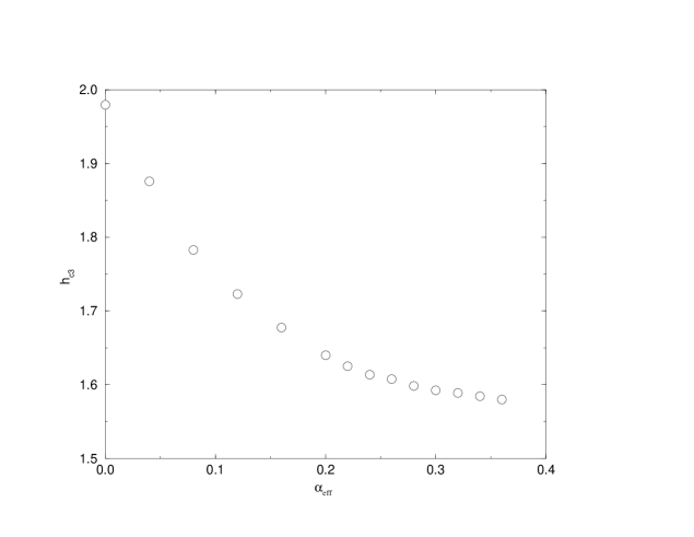
FIG. 13.: The upper critical field as a function of the defect strength.

VII Summary

Summarizing, we studied magnetic properties of mesoscopic superconducting discs with disordered attractive columnar defects. The number of defects is assumed to be larger than the maximal possible number of vortices accumulated by the disc. We obtained the magnetization curves for various strengths of defects in a wide region of the applied magnetic field. The results show that the defects help the penetration of vortices into the sample. They also reduce both the value of the magnetization and the upper critical field. Even the presence of weak defects can split the giant vortex state at the disc center (usually existing in a clean disc of small radius) into vortices with smaller topological charges. This splitting occurs in the vicinity of the upper critical field. Strong ehough defects always pin all vortices, splitting multiple vortex states at the disc center in all field region. This leads to the appearance of additional mesoscopic jumps in the magnetization curve related not to the penetration of new vortices into the sample but to redistribution of vortices within the set of defects. The number of these jumps enlarges increases with the number of defects.

VIII Acknowledgments

This research is supported by grants from the Israel Academy of Science “Mesoscopic effects in type II superconductors with short-range pinning inhomogeneities” (S.G.) and “Center of Excellence” (Y.A.) and by a DIP grant for German Israel collaboration (Y.A.).

REFERENCES

- [1] D. A. Brawner, N. P. Ong and Z. Z. Wang, Nature 358, 567 (1992);
- [2] A. K. Geim, I. V. Grigorieva and S. V. Dubonos, Phys. Rev. B 46, 324 (1992);
- [3] S. T. Stotdart, S. J. Bending, A. K. Geim and M. Henini, Phys. Rev. Lett. 71, 3854 (1993);
- [4] E. Zeldov, A. I. Larkin, V. B. Geshkenbein, M. Konczykowski, D. Majer, B. Khaykovich, V. M. Vinokur and H. Shtrikman Phys. Rev. Lett. 73, 1428 (1994);
- [5] A. K. Geim, S. V. Dubonos, J. G. S. Lok, I. V. Grigorieva, J. C. Maan, L. Theil Hansen and P. E. Lindelof, Appl. Phys. Lett. 71, 2379 (1997);
- [6] A. K. Geim, I. V. Grigorieva, S. V. Dubonos, J. G. S. Lok, J. C. Maan, A. E. Filippov and F. M. Peeters, Nature 390, 259 (1997);
- [7] P. Singha Deo, V. A. Schweigert, F. M. Peeters and A. K. Geim, Phys. Rev. Lett. 79, 4653 (1997);
- [8] V. A. Schweigert, F. M. Peeters and P. S. Deo, Phys. Rev. Lett. 81, 2783 (1998);
- [9] J. J. Palacios, Phys. Rev. B 58, R5948 (1998);
- [10] P. Singha Deo, F.M. Peeters, V.A. Schweigert, cond-mat/9812193 (1998);
- [11] E. Akkermans, K. Mallick, cond-mat/9812275 (1998);
- [12] L. Civale, A.D.Marwick, T.K. Worthington, M.A. Kirk, J.R. Thompson, L. Krusin-Elbaum, Y. Sun, J.R. Clem, F.H. Holtzberg, Phys. Rev. Lett. 67, 648 (1991);
- [13] C.J. van der Beek, M. Konczykowski, T.W. Li, P.H. Kes, W. Benoit, Phys. Rev. B 54, R792 (1996);
- [14] G. M. Braverman, S. A. Gredeskul, Y. Avishai, Phys. Rev. B, 57, 13899 (1998);
- [15] E.H. Brandt, Phys. Stat. Sol. (b) 51, 345 (1972);
- [16] I.S. Gradstein, and I.M. Ryzhik, Tables of Integtrals, Sums, Series and Products (Academic, New York, 1980);
- [17] Yu.N. Ovchinnikov, Sov. Phys. JETP 55, 1162 (1982);
- [18] R. Benoist and W. Zwerger, Z. Phys. B 103, 377 (1997);
- [19] D. Saint Jaims and P. G. De-Gennes, Phys. Lett. 7, 306 (1963).