Abstract

A two state (2-MO) model for the low-lying long axis-polarised excitations of poly(p-phenylene) oligomers and polymers is developed. First we derive such a model from the underlying Pariser-Parr-Pople (P-P-P) model of $\pi$-conjugated systems. The two states retained per unit cell are the Wannier functions associated with the valence and conduction bands. By a comparison of the predictions of this model to a four state model (which includes the non-bonding states) and a full P-P-P model calculation on benzene and biphenyl, it is shown quantitatively how the 2-MO model fails to predict the correct excitation energies. The 2-MO model is then solved for oligophenylenes of up to 15 repeat units using the density matrix renormalisation group (DMRG) method. It is shown that the predicted lowest lying, dipole allowed excitation is ca. 1 eV higher than the experimental result. The failure of the 2-MO model is a consequence of the fact that the original HOMO and LUMO single particle basis does not provide an adequate representation for the many body processes of the electronic system.

1 Introduction

Interest in the low-lying excitations of the phenyl based semiconductors, in particular poly(p-phenylene) and poly(p-phenylene vinylene), arises from the observation of their electroluminescence [1], [2] and the possibility of various optical and nonlinear devices. From a theoretical point of view one would like to understand how the excitations of the phenyl based semiconductors are derived from the parent excitations of benzene, how these evolve as a function of oligomer length, and how they participate in non-linear optical processes.

There is now a substantial body of experimental results on the photo- and electro- luminescent properties of poly(p-phenylene vinylene) [3, 4, 5, 6, 7, 8, 9, 10], and this has generated commicant theoretical interest [9, 11, 12, 13, 14]. Fewer experimental results exist for poly(p-phenylene) [15, 16, 17, 2, 18], however, largely resulting from the difficulties in obtaining well characterised material. There have been a number of theoretical calculations on poly(p-phenylene). Brédas has used the VEH pseudopotential technique [19] and Ambrosch-Draxl et al. have performed density functional calculations using LAPW and pseudopotentials [16]. Rice et al. [13] have developed a phenomenological, microscopic model based on the molecular excitations of benzene. The absorption bands are calculated using an approximate Kubo formalism.

In this paper we will restrict our attention to poly(p-phenylene), and develop in full detail the model and computational techniques introduced in a recent letter [20], [21]. Our goal is to construct a model of poly(p-phenylene) based on the underlying Pariser-Parr-Pople (P-P-P) model of $\pi$-conjugated electron systems [22]. The P-P-P model has long been used to describe the low-lying excitations of $\pi$-conjugated systems, giving reasonable results. However, an improved parameterisation of this model is possible, and that was achieved in a previous paper [23]. We will use this optimised parameterisation in the current paper. We will show, at the very least, that to achieve our goal of a full description of poly(p-phenylene) a four molecular orbital (4-MO) model (as described below) is required. However, in this paper our ambition will be more limited, and we will primarily be concerned with a description of the long axis-polarised excitations. One of the aims of this paper is to show how well the 2-MO model, whose parameters are directly obtained from the underlying P-P-P model, explains the physics of the oligophenylenes. This will be done by comparing the predictions of the 4-MO and 2-MO models to exact P-P-P calculations of benzene and biphenyl. By systematically reducing the size of the Hilbert space we will show how the discrepencies between the full and reduced models arise. Next, equipped with the knowledge of how well the 2-MO model predicts the biphenyl excitations, we solve oligophenylenes of up to 15 repeat units using the density matrix renormalisation group (DMRG) method. This technique is ideally suited to solving lattice quantum Hamiltonians with open boundary conditions. We find that the theoretical predictions of the exciton energies are ca. 1 eV higher than the experimental results. We argue that failure of the 2-MO model is a consequence of the fact that the original HOMO and LUMO single particle basis does not provide an adequate representation for the many body processes of the electronic system.

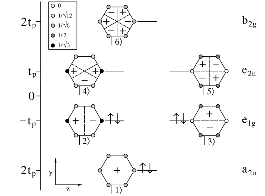
Figure 1: Molecular orbitals of phenylene, the repeat unit of poly(p-phenylene). The amplitude of the wavefunction is indicated by shading. The dashed lines are the nodes of the wavefunction.

The molecular orbital approach to the study of conjugated polymers is not new. Recently it has been used by Soos et al. [24] on their work on the phenyl semiconductors, while Chandross et al. employed a similar approach in their work on conjugated polymers [25].

The plan of this paper is as follows. First, the 4-MO and 2-MO models of benzene and oligophenylenes (including biphenyl) will be introduced. By making direct comparison between the full 6-MO calculation of benzene and biphenyl we will show the successes and limitations of these reduced models. Next, we solve the 2-MO model to describe the low energy physics of the oligophenylenes. Finally, section 6 concludes.

2 The Molecular Orbital Approach

2.1 The Four-Molecular Orbital (4-MO) Model

The essential repeat unit of oligophenylenes is the phenylene repeat unit. Its one-electron atomic orbital basis may be more conveniently represented as a one-electron molecular orbital basis, which is the set of eigenstates of the phenylene kinetic energy operator. These are illustrated in Fig. 1 as eigenstates of the $x$-$y$ and $x$-$z$ plane reflection operators (i.e. $\hat{\sigma}(xy)$ and $\hat{\sigma}(xz)$). Solving the P-P-P model within the full 6-MO basis is of course equivalent to solving within the full atomic orbital basis. However, keeping such a large number of states within an exact calculation soon becomes prohibitively expensive in memory and cpu time resources. The largest oligophenylene which can be solved exactly is biphenyl. Even with sophisticated Hilbert space truncation procedures, such as the DMRG method, there are technical reasons why it is difficult to retain the full 6-MO, or even the 4-MO, basis.

In addition to the technical difficulties of retaining the full 6-MO basis, one might suppose that the low-lying excitations arise between the MO states closest to the Fermi energy, and that these alone are sufficient to describe the low energy physics of oligophenylenes. In this approach, the MOs furthest from the Fermi energy remain frozen. In benzene, for example, the MOs which are retained are the $e_{u}$ and $e_{g}$ states, while the $a_{u}$ and $b_{g}$ states are frozen. In biphenyl, extended MOs are formed, and, by Fourier transforming the extended orbitals, we construct localised (Wannier) orbitals. The eight Wannier orbitals which are retained are those associated with the eight biphenyl MOs closest to the Fermi energy.

2.2 The Two-Molecular Orbital (2-MO) Model

The 2-MO model reduces the Hibert space yet further by retaining only a pair of states per repeat unit. In benzene, four calculations are performed, corresponding to the various pairings of the bonding ($|2\rangle$ and $|4\rangle$) and non-bonding ($|3\rangle$ and $|5\rangle$) orbitals. In biphenyl it is either the Wannier orbitals associated with the bonding biphenyl MOs or the non-bonding orbitals. Likewise, in long oligophenylenes, the extended MOs form bands, as shown in Fig. 2 for an infinite chain with periodic boundary conditions. By Fourier transforming the Bloch states associated with the valence and conduction bands we obtain the pair of relevant Wannier orbitals required to describe the low energy physics, as shown in Appendix A [26]. The reason why this might appear to be a reasonable assumption for the consideration of the $1^{1}B_{1u}$ exciton of oligophenylenes will be discussed in more detail shortly.

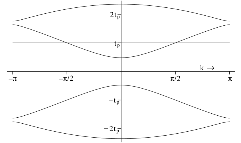
Figure 2: Non-interacting band structure of poly(p-phenylene).

3 Benzene

In this section we compare the predictions of the 4-MO and 2-MO models to the full (6-MO) P-P-P model calculation of benzene.

The P-P-P Hamiltonian is written as

$$H=-\sum_{<ij>\,\sigma}t_{ij}\left[c_{i\sigma}^{\dagger}c_{j\sigma}+\rm{h.c.}\right]+U\sum_{i}\left(n_{i\uparrow}-\frac{1}{2}\right)\left(n_{i\downarrow}-\frac{1}{2}\right)+\frac{1}{2}\sum_{i\neq j}V_{ij}(n_{i}-1)(n_{j}-1),$$ (1)

where $c_{i\sigma}^{\dagger}$ creates a $\pi$ electron with spin $\sigma$ on carbon site $i$, $n_{i\sigma}=c_{i\sigma}^{\dagger}c_{i\sigma}$, $n_{i}=n_{i\uparrow}+n_{i\downarrow}$ and $<>$ represents nearest neighbours.

We use the Ohno parameterisation for the Coulomb interaction [27],

$$V_{ij}=\frac{U}{(1+\alpha r_{ij}^{2})^{1/2}},$$ (2)

where $\alpha=(U/14.397)^{2}$, thus ensuring that $V_{ij}\rightarrow e^{2}/(4\pi\epsilon_{0}r_{ij})$ as $r_{ij}\rightarrow\infty$, and $r_{ij}$ is the inter-atomic distance in Å. The C-C bond length is taken as 1.40 Å. The optimal parameterisation, which was derived in [23], is $U=10.06$ eV and the phenyl bond transfer integral, $t_{\mbox{\scriptsize p}}=2.539$ eV.

The MO representation diagonalises the kinetic energy operator at the expense of introducing off-diagonal, two-electron terms into the interactions. In this representation the Hamiltonian reads

$$H=\sum_{\alpha=1}^{6}\epsilon_{\alpha}(n_{\alpha}-1)+\frac{1}{4}\sum_{\alpha\beta\gamma\delta\sigma\sigma^{\prime}}V_{\alpha\beta\gamma\delta}(a^{\dagger}_{\alpha\sigma}a^{\dagger}_{\gamma\sigma^{\prime}}a_{\delta\sigma^{\prime}}a_{\beta\sigma}+a_{\bar{\alpha}\bar{\sigma}}a_{\bar{\gamma}\bar{\sigma^{\prime}}}a^{\dagger}_{\bar{\delta}\bar{\sigma^{\prime}}}a^{\dagger}_{\bar{\beta}\bar{\sigma}}),$$ (3)

where

$$V_{\alpha\beta\gamma\delta}=\int\int d^{3}{\bf r}_{1}d^{3}{\bf r}_{2}\,\psi^{\ast}_{\alpha}({\bf r}_{1})\psi_{\beta}({\bf r}_{1})\frac{e^{2}}{4\pi\epsilon_{0}|{\bf r}_{1}-{\bf r}_{2}|}\psi^{\ast}_{\gamma}({\bf r}_{2})\psi_{\delta}({\bf r}_{2}),$$ (4)

$a_{\alpha\sigma}^{\dagger}$ creates an electron of spin $\sigma$ in the MO $\left|\alpha\right\rangle$ and $\epsilon_{\alpha}$ are the MO eigenvalues. Eqn. (3) is invariant under the particle-hole transformation $a^{\dagger}_{\alpha\sigma}\leftrightarrow{\rm sgn}(\sigma)a_{\bar{\alpha}\bar{\sigma}}$ where the MOs transform as $\left|\bar{1}\right\rangle$ = $\left|6\right\rangle$, $\left|\bar{2}\right\rangle$ = $\left|4\right\rangle$ and $\left|\bar{3}\right\rangle$ = $\left|5\right\rangle$.

Inserting

$$\psi_{\alpha}({\bf r}_{1})=\sum_{i}f^{\alpha}_{i}\phi_{i}({\bf r}_{1}),$$ (5)

where $\phi_{i}({\bf r}_{1})$ are the orthogonalised atomic orbitals, and using

$$\int\int d^{3}{\bf r}_{1}d^{3}{\bf r}_{2}\,\phi^{\ast}_{i}({\bf r}_{1})\phi_{i^{\prime}}({\bf r}_{1})\frac{e^{2}}{4\pi\epsilon_{0}|{\bf r}_{1}-{\bf r}_{2}|}\phi^{\ast}_{j}({\bf r}_{2})\phi_{j^{\prime}}({\bf r}_{2})=V_{ij}\delta_{ii^{\prime}}\delta_{jj^{\prime}}$$ (6)

gives

$$V_{\alpha\beta\gamma\delta}=\sum_{ij}f^{\alpha}_{i}f^{\beta}_{i}V_{ij}f^{\gamma}_{j}f^{\delta}_{j}.$$ (7)

Table 1 lists the two-electron integrals used in the benzene calculation. All the two-electron integrals are retained in the 6-MO calculation to reproduce the atomic orbital basis calculation of [23].

2-e parameter	Name	Benzene	Biphenyl	Oligophenylenes
$V_{\alpha\alpha\alpha\alpha}$	‘Onsite’ Coulomb	Yes	Yes	Yes
$V_{\alpha\alpha\beta\beta}$	Direct Coulomb	Yes	Yes	Yes
$V_{\alpha\beta\beta\alpha}$	Exchange	Yes	Yes	Yes
$V_{\alpha\beta\alpha\beta}$	Pair hop	Yes	Yes	Yes
$V_{\alpha\alpha\alpha\beta}$	Effective hopping	Yes	Yes	No
$V_{\alpha\alpha\beta\gamma}$	Effective hopping	Yes	Yes	No
$V_{\alpha\beta\alpha\gamma}$	3-centre	Yes	Yes	No
$V_{\alpha\beta\gamma\alpha}$	3-centre	Yes	Yes	No
$V_{\alpha\beta\gamma\delta}$	4-centre	Yes	Yes	No

Table 1: The two-electron parameters used in the MO Hamiltonian, Eq. (3).

A reduced symmetry of the benzene Hamiltonian is invariance under reflection in the $x$-$y$ and $x$-$z$ planes. The MO basis, Fig. 1, possesses this symmetry and partly diagonalises the many body Hamiltonian (3). In particular, the states arising from excitations between (predominately) $\left|2\right\rangle\rightarrow\left|4\right\rangle$ and $\left|3\right\rangle\rightarrow\left|5\right\rangle$ mix and are odd under $\hat{\sigma}(xy)$ and even under $\hat{\sigma}(xz)$ reflection. These become the $1B_{1u}$ and $1E_{1u}(z)$ states. Similarly, the states arising from excitations between (predominately) $\left|2\right\rangle\rightarrow\left|5\right\rangle$ and $\left|3\right\rangle\rightarrow\left|4\right\rangle$ mix and are odd under $\hat{\sigma}(xz)$ and even under $\hat{\sigma}(xy)$ reflection, and these become the $1B_{2u}$ and $1E_{1u}(y)$ states.

State	$\sigma(xy)$	$\sigma(xz)$	6-MO	4-MO	2-MO	Experiment
$1^{1}B^{+}_{2u}$	$+$	$-$	4.75	5.55	6.34	4.90
$1^{1}B^{-}_{1u}$	$-$	$+$	5.47	5.71	6.43	6.20
$1^{1}E^{-}_{1u}(z)$	$-$	$+$	6.99	7.34	6.43	6.94
$1^{1}E^{-}_{1u}(y)$	$+$	$-$	6.99	7.34	6.34	6.94
$1^{3}B^{+}_{1u}$	$-$	$+$	4.13	4.68	4.73	3.94
$1^{3}E^{+}_{1u}(z)$	$-$	$+$	4.76	5.24	4.73	4.76
$1^{3}E^{+}_{1u}(y)$	$+$	$-$	4.76	5.24	5.08	4.76
$1^{3}B^{-}_{2u}$	$+$	$-$	5.60	5.55	5.08	5.60

Table 2: Full P-P-P (6-MO), 4-MO and 2-MO model calculations of the vertical, low-lying excitations of benzene in eV. Also listed are the experimental vertical, low-lying transitions from [28].

Table 2 lists the results of the 6-MO (full) and the 4-MO calculation. The full 6-MO basis, using the optimised parameters derived in [23], results in an average error of 2.75%. The ordering of the states is consistent with experiment, except for the $1^{1}B_{2u}$ state, which lies just above the $1^{3}E_{1u}$ state experimentally, while theoretically the ordering is reversed. However, the energy of the $1^{1}B_{1u}$ state is over $0.7$ eV too low [29].

The discrepencies between the full calculation and the 4-MO results are reasonable (particularly for the dominant singlet excitations, $1^{1}E_{1u}$), being of the order of a few tenths of an eV. The 4-MO calculation, however, does predict that the singlet and triplet $1B_{2u}$ states are degenerate, whereas experimentally the singlet lies below the triplet.

The results of the 2-MO calculations are also shown. The $\left|2\right\rangle\rightarrow\left|4\right\rangle$ and $\left|3\right\rangle\rightarrow\left|5\right\rangle$ excitations decouple and are degenerate, and likewise with the $\left|2\right\rangle\rightarrow\left|5\right\rangle$ and $\left|3\right\rangle\rightarrow\left|4\right\rangle$ excitations. As expected, there are substantial deviations with these results from the full calculation. This results from the absence of mixing between the states. However, for oligophenylenes, the bonding HOMO and LUMO states will begin to form bands, thus lifting the degeneracy between the bonding and non-bonding orbitals, and hence the mixing will reduce. Thus, for oligomers the 2-MO model may result in smaller discrepancies. To investigate this assumption, we now turn to a discussion of biphenyl.

4 Biphenyl

The accuracy of the 4-MO and 2-MO models as applied to biphenyl will give some indication of their reliability for longer oligophenylenes. As in benzene, the 4-MO model uses four states per repeat unit. However, rather than use the primitive benzene MOs, we construct Wannier MOs obtained by Fourier transforming the biphenyl molecular orbitals. A full description of this procedure is left to Appendix A, where Wannier MOs are derived for a system with periodic boundary conditions.

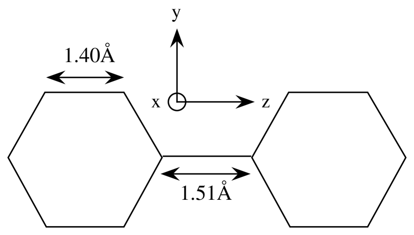
Figure 3: Chemical structure of biphenyl showing the bond lengths used in our calculation.

Biphenyl belongs to the $D_{2h}$ symmetry group. We adopt the convention that the $z$-axis is the long axis and the $y$-axis is the short axis, as shown in Fig. 3, along with the bond lengths used in our calculation. The optimised parameterisation for $U$ and $t_{\mbox{\scriptsize p}}$ are those derived in [23] and used in section 3. The single bond hybridisation integral, $t_{\mbox{\scriptsize s}}$, is also determined empirically by fitting the theoretical calculation to the experimental $1^{1}B_{1u}$ exciton at $4.80$ eV in biphenyl crystals. This gives $t_{\mbox{\scriptsize s}}=2.22$ eV.

State	$\sigma(xy)$	$\sigma(xz)$	6-MO	4-MO	2-MO	Experiment
$1^{1}B^{+}_{2u}$	$+$	$-$	4.55	5.35	NA	4.20 (0-0)–4.49
$1^{1}B^{+}_{3g}$	$-$	$-$	4.58	5.40	NA	4.11 (0-0)
$1^{1}B^{-}_{1u}$	$-$	$+$	4.80	5.25	5.46	4.80
$2^{1}A^{-}_{g}$	$+$	$+$	5.57	5.85	6.80	4.71–5.02
$2^{1}B^{-}_{1u}$	$-$	$+$	6.22	6.59	6.43	6.14, 6.16
$2^{1}B^{-}_{3g}$	$-$	$-$	6.28	6.80	NA	—
$3^{1}A^{+}_{g}$	$+$	$+$	6.30	7.19	7.14	ca. 6.0 (max)
$2^{1}B^{-}_{2u}$	$-$	$+$	6.66	7.17	NA	5.85, 5.96
$1^{3}B^{+}_{1u}$	$-$	$+$	3.63	4.29	4.42	ca. 3.5 (max)
$1^{3}A^{+}_{g}$	$+$	$+$	4.25	4.84	5.13	—
$2^{3}B^{+}_{1u}$	$-$	$+$	4.56	5.06	4.73	—
$1^{3}B^{+}_{2u}$	$+$	$-$	4.56	5.10	NA	3.93 (0-0)
$1^{3}B^{+}_{3g}$	$-$	$-$	4.56	5.10	NA	—
$2^{3}A^{+}_{g}$	$+$	$+$	4.80	5.35	4.73	—
$2^{3}B^{-}_{2u}$	$+$	$-$	5.32	5.42	NA	—
$2^{3}B^{-}_{3g}$	$-$	$-$	5.37	5.47	NA	—

Table 3: Full P-P-P (6-MO), 4-MO and 2-MO model calculations of the low-lying excitations of biphenyl in eV. The experimental results are described in [23].

Table 3 shows the full P-P-P biphenyl calculation and the corresponding experimental results. A full comparison of theory and experiment is presented in ref. [23], so here we merely summarise the results. The P-P-P calculation is very successful in its predictions of the long axis-polarised singlet and triplet states. It is less succesful, however, in its treatment of the short axis-polarised states. For example, it predicts that the $2^{1}B_{2u}$ state is higher than the $2^{1}B_{1u}$ state and that the $1^{1}B_{3g}$ state lies higher than the $1^{1}B_{2u}$ state, both of which are in contradiction to experiment. In [23] we argued that this discrepency is a consequence of the neglect of next nearest neighbour hopping in the P-P-P model.

Now let us compare the predictions of the 4-MO and 2-MO model calculations to the full calculation. As shown in table 3 the most obvious discrepency between the 4-MO and full calculations is that the former predicts that the $1^{1}B^{-}_{1u}$ state lies below the $1^{1}B^{+}_{3g}$ and $1^{1}B^{+}_{2u}$ states. In addition, all the energies are too high: the $1^{1}B^{-}_{1u}$ state is predicted at 0.45 eV (i.e. 9%) higher than the full calculation. The ordering of the states in the triplet sector agrees with the full calculation, but again they ca. 0.5 eV too high. This poor agreement between the 6-MO and 4-MO calculations indicates the importance of electronic correlations between the eight active orbitals (i.e. the HOMO and LUMO) and the four frozen orbitals (i.e. those furthest from the Fermi energy). The neglect of the strong mixing of these frozen states in the 4-MO calculation results in both quantitative and qualitative discrepencies.

Table 3 also shows the results of the 2-MO calculation for the long axis-polarised states. It is noteworthy that the discrepencies between the 2-MO and 4-MO calculations are smaller than those between the 4-MO and 6-MO calculation, and results from the fact that electronic correlations between the active orbitals are smaller than those between the active and frozen orbitals. However, the 2-MO basis is clearly not capable of predicting accurate energies for the key excitations in biphenyl. The errors from the 6-MO calculation for the $1^{3}B_{1u}$, $1^{1}B_{1u}$ and $3^{1}A_{g}$ states are 20%, 13% and 12%, respectively.

Before turning to a discussion of the 2-MO calculation for oligophenylenes, let us use the biphenyl results to predict the main features of the optical excitations in oligophenylenes. First, the excitations are either $z$- or $y$- polarised states. The $z$-polarised states are derived from the $1^{1}B^{-}_{1u}$ and $1^{1}E^{-}_{1u}(z)$ parent states of benzene. The former of these is dipole forbidden, but in forming delocalised states these excitations mix and oscillator strength is transfered from the high energy excitation to the low energy excitation. The lowest state becomes the $1^{1}B^{-}_{1u}$ exciton, and arises predominately from excitations between molecular orbital valence and conduction bands. The highest energy excitation becomes the localised (or non-bonding) exciton at ca. 6.2 eV, and results from excitations between the non-bonding bands. In the next section we will be attempt to describe these two excitations within a 2-MO model.

The $y$-polarised states are derived from the $1^{1}B_{2u}^{+}$ and $1^{1}E_{1u}^{-}(y)$ excitations of benzene. These excitations do not mix in oligophenylenes, and the former state is expected to result in the weakly particle-hole allowed feature at 4.5 eV, while the latter results in the stronger absorption at 5.5 eV [13].

5 Oligophenylenes: The Wannier 2-MO Model

In the absence of electronic correlations, the lowest long axis-polarised, dipole allowed state would be a transition between the molecular orbital valence and conduction bands depicted in Fig. 2. The high energy non-bonding exciton arises from transitions between the non-bonding orbitals. Turning on the correlations leads to a mixing of the single particle basis which, as shown earlier in this paper, leads to both quantitative and qualitative corrections. In this section, however, we assume that the low-lying excitations may be described entirely within the 2-MO subspace associated with the valence and conduction bands. The localised Wannier MOs, which are used to calculate the two-electron parameters, are obtained by Fourier transforming the Bloch functions associated with these bands. Such Wannier MOs are not only delocalised over neighbouring phenylene rings, but they also contain an admixture of different primitive phenylene MOs. They retain, however, the same spatial symmetry as their corresponding primitive phenylene MOs.

Parameter	Name	Wannier-MO
U	Onsite Coulomb repulsion	5.687
V	Nearest neighbour Coulomb repulsion	3.612
X	Onsite exchange	0.581
P	Onsite pair hop	0.581
$\Delta^{*}$	HOMO-LUMO gap	5.462
$t_{11}=-t_{22}$	Nearest neighbour hybridisation	0.667
$t_{12}=-t_{21}$	Nearest neighbour hybridisation	0.0

Table 4: The parameters and their values in eV used in the 2-MO model (Eq. 8) for oligophenylenes. $*$ Includes static Coulomb terms from the frozen electrons.

The procedure for obtaining these Wannier orbitals is described in Appendix A. The two-electron parameters retained in the Hamiltonian and their values are shown in table 4, along with the renormalised one-electron integrals. Notice that the three and four centre Coulomb terms are neglected for the oligomer calculation as they have little effect on the results. The interactions which will go into the model are: the HOMO-LUMO gap, direct onsite and nearest neighbour MO Coulomb repulsion, spin-exchange and pair hop between MOs on the same repeat unit, and hopping between neighbouring repeat units. These parameters are the minimum required to model the formation and delocalisation of singlet and triplet excitons along the poly(p-phenylene) backbone. The 2-MO model Hamiltonian is thus,

$$H = -\sum_{i\,\alpha\,\beta\,\sigma}t_{\alpha\beta}\left[a_{i\alpha\sigma}^{\dagger}a_{i+1\beta\sigma}+\rm{h.c.}\right]+\sum_{i\,\alpha}\epsilon_{\alpha}(n_{i\alpha}-1)+U\sum_{i\,\alpha}\left(n_{i\alpha\uparrow}-\frac{1}{2}\right)\left(n_{i\alpha\downarrow}-\frac{1}{2}\right)$$ (8)

$$+\;\frac{U}{2}\sum_{i\,\alpha\neq\beta}(n_{i\alpha}-1)(n_{i\beta}-1)+V\sum_{i\,\alpha\,\beta}(n_{i\alpha}-1)(n_{i+1\beta}-1)$$

$$-\;X\sum_{i\,\alpha\neq\beta}\left[{\mbox{\boldmath$S$}}_{i\alpha}.{\mbox{\boldmath$S$}}_{i\beta}+\frac{1}{4}\left(n_{i\alpha}-1\right)\left(n_{i\beta}-1\right)\right]$$

$$+\;\frac{P}{2}\sum_{i\,\alpha\neq\beta\,\sigma}a_{i\alpha\sigma}^{\dagger}a_{i\alpha\bar{\sigma}}^{\dagger}a_{i\beta\bar{\sigma}}a_{i\beta\sigma},,$$

where, ${\mbox{\boldmath$S$}}_{i\alpha}=\sum_{\rho\rho^{\prime}}a_{i\alpha\rho}^{\dagger}{\mbox{\boldmath$\sigma$}}_{\rho\rho^{\prime}}a_{i\alpha\rho^{\prime}}$ and $\sigma$ are the Pauli spin matrices.

Eq. 8 is solved exactly for oligomers of up to six repeat units using the conjugate gradient method. For longer oligomers of up to 15 units we use the density matrix renormalisation group method [32, 33]. The DMRG is a powerful, robust, portable and highly accurate truncated basis scheme for the solution of low dimensional quantum lattice systems, and is especially well suited to the solution of open linear chains such as (8). Since the method is discussed at length in [32] and reviewed in [33] we restrict ourselves here to a discussion of the specifics of our implementation for (8).

In addition to the total charge $\hat{N}=\sum_{i\,\alpha}n_{i\alpha}$ and the total $z$-spin $\hat{S}^{z}_{\mbox{\scriptsize T}}=\frac{1}{2}\sum_{i\,\alpha}\left(n_{i\alpha\uparrow}-n_{i\alpha\downarrow}\right)$, the spatial inversion ($\hat{C}_{2}$: $a_{i\alpha\sigma}\mapsto a_{L-i+1\,\alpha\sigma}$), particle-hole ($\hat{J}$: $a_{i1\sigma}^{\dagger}\mapsto{\rm sgn}(\sigma)a_{i2\bar{\sigma}}$, $a_{i2\sigma}^{\dagger}\mapsto{\rm sgn}(\sigma)a_{i1\bar{\sigma}}$) and spin flip ($\hat{P}$: $a_{i\alpha\sigma}\mapsto a_{i\alpha{\bar{\sigma}}}$) symmetry operators are used as good quantum numbers in diagonalising the Hamiltonian. We verify the validity of the DMRG solution by checking that the results obtained for the trimer and the pentamer agree with exact diagonalisation results. Basis truncation occurs for larger chains. We retain $m=210$ states per block in our calculations. We test the convergence of the truncation scheme by examining the non-interacting ($U=V=X=P=0$) case which can easily be diagonalised exactly for any chain length. We have found that the DMRG resolves gaps between these states well and truly above the accuracy required in order to make comparisons with experiments, that is, a few hundreds of an eV. The accuracy is even better in the interacting case where states are more localised and gaps are widened [32]. A systematic analysis of the convergence of energies in (8) is presented elsewhere [31].

Table 5 shows the energies of the vertical transitions as a function of oligomer length of the $1^{3}B_{1u}^{+}$, the $1^{1}B_{1u}^{-}$ and the lowest even, covalent excitation, which we label as $m^{1}A^{+}_{g}$. Notice that, in general, the $m^{1}A^{+}_{g}$ is not the lowest $A_{g}$ excitation. For example, in biphenyl, it corresponds to the $3^{1}A^{+}_{g}$ state; there being an ionic $A_{g}$ state below it. Furthermore, it is not necessarily the state with the largest oscillator strength with the $1^{1}B_{1u}^{-}$ state. Also shown are the experimental results for crystalline thin films. Evidently, for longer oligomers, for which the Wannier parameterisation should be the most appropriate, the theoretical predictions are ca. 1 eV too high. Although these results are not unreasonable, we nonetheless conclude that a 2-MO model, whose parameters are obtained directly form the underlying P-P-P model, is incapable of quantitative predictions of the low-lying exciton energies.

$L$	$1^{1}B^{-}_{u}$	$m^{1}A^{+}_{g}$	$1^{3}B^{+}_{u}$	Experimental Optical Gap
2	5.13	7.02	4.27	4.80(a)
3	4.79	6.79	3.99	4.5(b)
4	4.66	6.66	3.88	—
5	4.59	6.61	3.83	—
6	4.56	6.58	3.80	3.9(b)
7	4.52	6.56	3.78	—
11	4.51	6.54	3.76	—
13	4.50	6.54	3.75	—
15	4.50	6.54	3.75	—
$\infty$	4.50	6.54	3.75	3.43(b), 3.3(c), 3.5(d)

Table 5: Calculated vertical transition energies in eV for oligophenylenes of various lengths, $L$, using the Wannier MO parameters. Note that the $m^{1}A^{+}_{g}$ exciton is the lowest covalent $A_{g}$ singlet excited state. Experimental results from biphenyl crystals (a) [34] and crystalline films (b) [17], (c) [15], (d) [16].

In the 2-MO model excitations between the valence and conduction bands and between the non-bonding orbitals are decoupled. As described above, the former leads to the $1^{1}B_{1u}$ exciton, while the latter results in the non-bonding exciton. The energy of this exciton can therefore be estimated: it is the energy of the singlet benzene exciton predicted by the 2-MO model in section 3. This is $6.43$ eV, which is quite close to the experimental value of ca. $6.2$ eV.

6 Conclusions

In this paper we have developed a recently introduced two state (2-MO) model for the low-lying, long axis-polarised excitations of poly(p-phenylene) oligomers and polymers. We have shown that a 2-MO model, based on the HOMO and LUMO states, can be derived from the underlying Pariser-Parr-Pople (P-P-P) model by freezing out those orbitals further from the Fermi energy. By a careful comparison of the predictions of the 4-MO and 2-MO models to the exact P-P-P results for benzene and biphenyl we have shown quantitatively how the 2-MO model fails to predict excitation energies. For example, it predicts the $1^{1}B_{1u}$ exciton to be 0.66 eV (13%) higher than the exact P-P-P calculation in biphenyl.

Next, we have solved the 2-MO model, where the MOs are Wannier orbitals obtained by Fourier transforming the Bloch states associated with the valence and conduction bands of poly(p-phenylene) polymers, for oligophenylenes of up to 15 repeat units using the DMRG method. We showed that these parameters lead to an over estimation of the $1^{1}B_{1u}$ exciton by ca. $1$ eV in comparison with experiment.

Thus, both a comparison of the 2-MO model to full P-P-P calculations and to experiment shows that it quantitatively fails to predict the excitation energies. The reason for these discrepencies lies in the fact that the original HOMO and LUMO single particle basis does not provide an adequate representation for the many body processes of the electronic system. Thus, the orbitals which are assumed to be frozen in the 2-MO model in fact participate dynamically in the many body states. To incorporate this effect, one can assume that a two state model, with the relevant many body interactions, is appropriate to describe the low energy physics, but that these parameters are renormalised from their bare P-P-P values. The aim is to parameterise a two state model by fitting its predictions to the exact P-P-P model calculations of benzene and biphenyl. If a robust parameterisation of oligophenylenes can be achieved, by which we mean a reasonably accurate prediction of exciton energies, then other quantities, such as oscillator strengths, non-linear optical coefficients and correlation functions can be calculated with some confidence. This is the subject of [31].

R.J.B. acknowledges the support of the Australian Research Council. The DMRG calculations were performed on the SGI Power Challenge facility at the New South Wales Centre for Parallel Computing. W.B. acknowledges financial support from the EPSRC (U.K.) (GR/K86343), and thanks Dr. M. Yu. Lavrentiev for useful discussions. H.D. is supported by an EPSRC studentship.

Appendix A Wannier Orbitals

The Bloch states associated with the band $j$ with energy $\epsilon_{k}^{j}$ are

$$\left|\psi_{k}^{j}\right\rangle=\sum_{\alpha}u_{k}^{j\alpha}\left|\psi_{k}^{\alpha}\right\rangle$$ (A.1)

where $\sum_{\alpha}u_{k}^{j\alpha}$ is the eigenvector.

$\left|\psi_{k}^{\alpha}\right\rangle$ is the Fourier transform of the $\alpha$ phenylene molecular orbital state, i.e.

$$\left|\psi_{k}^{\alpha}\right\rangle=\frac{1}{\sqrt{N}}\sum_{n=1}^{N}\left|\psi_{n}^{\alpha}\right\rangle e^{ikn}.$$ (A.2)

Likewise, the Wannier function associated with the $j$th Bloch state is,

$$\left|\psi_{n}^{j}\right\rangle=\frac{1}{\sqrt{N}}\sum_{n=1}^{N}\left|\psi_{k}^{j}\right\rangle e^{-ikn}.$$ (A.3)

Substituting (A1) and (A2) into (A3) gives

$$\left|\psi_{n}^{j}\right\rangle=\sum_{m}\sum_{\alpha}\tilde{u}_{m}^{j\alpha}\left|\psi_{n+m}^{\alpha}\right\rangle,$$ (A.4)

where $\tilde{u}_{m}^{j\alpha}$ is the Fourier transform of $u_{k}^{j\alpha}$, i.e.

$$\tilde{u}_{m}^{j\alpha}=\frac{1}{N}\sum_{k}u_{k}^{j\alpha}e^{ikm}.$$ (A.5)

The one-electron integrals are easily obtained within the Wannier MO basis. We require

$$t_{mn}^{j^{\prime}j}=\left\langle\psi_{m}^{j^{\prime}}\right|{\cal H}_{1-e}\left|\psi_{n}^{j}\right\rangle.$$ (A.6)

Now, using (A3)

$${\cal H}_{1-e}\left|\psi_{n}^{j}\right\rangle=\frac{1}{\sqrt{N}}\sum_{k}\epsilon_{k}^{j}\left|\psi_{k}^{j}\right\rangle e^{-ikn}$$ (A.7)

and by virtue of the orthogonality of the Bloch states, i.e.

$$\left\langle\psi_{k^{\prime}}^{j^{\prime}}\left|\psi_{k}^{j}\right.\right\rangle=\delta_{k^{\prime}k}\delta_{j^{\prime}j}$$ (A.8)

$$t_{mn}^{j^{\prime}j}=\frac{1}{N}\delta_{j^{\prime}j}\sum_{k}\epsilon_{k}^{j}e^{ik(m-n)}.$$ (A.9)

The two-electron integrals are more easily calculated by using the real space representation and inserting the Ohno interaction, as described in section 3.

References

- [1] J. H. Burroughes, D. D. C. Bradley, A. R. Brown, R. N. Marks, K. McKay, R. H. Friend, P. L. Burns and A. B. Holmes, Nature (London) 347 (1990) 539.
- [2] M. Klemenc, F. Meghdadi, S. Voss and G. Leising, Synth. Met. 85 (1997) 1243.
- [3] D. A. Haliday, P. L. Burn, R. H. Friend, D. D. C. Bradley, A. B. Holmes and A. Kraft, Synth. Met. 55–57 (1993) 954.
- [4] H. S. Woo, O. Lhost, S. C. Graham, D. D. C. Bradley, R. H. Friend, C. Quattrocchi, J. L. Brédas, R. Schenk and K. Müllen, Synth. Met. 59 (1993) 13.
- [5] S. Heun, R. F. Mahrt, A. Greiner, U. Lemmer, H. Bässler, D. A. Haliday, D. D. C. Bradley, P. L. Burn and A. B. Holmes, J. Phys. C 5 (1993) 247.
- [6] K. Pichler, D. A. Haliday, D. D. C. Bradley, P. L. Burn, R. H. Friend and A. B. Holmes, J. Phys. C 5 (1993) 7155.
- [7] C. H. Lee, G. Yu and A. J. Heeger, Phys. Rev. B 47 (1993) 15 543.
- [8] J. M. Leng, S. Jeglinski, X. Wei, R. E. Benner, Z. V. Vardeny, F. Guo and S. Mazumdar, Phys. Rev. Lett. 72 (1994) 156.
- [9] M. Chandros, S. Mazumdar, S. Jeglinski, X. Wei, Z. V. Vardeny, E. W. Kwock and T. M. Miller, Phys. Rev. B 50 (1994) 14 702.
- [10] R. Kersting, U. Lemmer, M. Deussen, H. J. Bakker, R. F. Mahrt, H. Kurz, V. I. Arkhipov, H. Bässler and E. O. Göbel, Phys. Rev. Lett. 73 (1994) 1440.
- [11] D. Beljionne, Z. Shuai, R. H. Friend and J. L. Brédas, J. Chem. Phys. 102 (1995) 2042.
- [12] F. Guo, M. Chandros and S. Mazumdar, Phys. Rev. Lett. 74 (1995) 2086.
- [13] Yu. N. Gartstein, M. J. Rice and E. M. Conwell, Phys. Rev. B 52 (1995) 1683.
- [14] Y. Shimoi and S. Abe, Synth. Met. 78 (1996) 219.
- [15] B. Tieke, C. Bubek and G. Lieser, Makroml. Chem. Rapid Comm. 3 (1982) 261.
- [16] C. Ambrosch-Draxl, J. A. Majewski, P. Vogl and G. Leising, Phys. Rev. B 51 (1995) 9668.
- [17] L. W. Shacklette, H. Eckhardt, R. R. Chance, G. G. Miller, D. M. Ivory and R. H. Baughman, J. Chem. Phys. 73 (1980) 4098.
- [18] S. Tasch, A. Niko, G. Leising and U. Scherf, Appl. Phys. Lett. 68 (1996) 1090.
- [19] J. L. Brédas, J. Chem. Phys. 82 (1985) 3808.
- [20] W. Barford and R. J. Bursill, Chem. Phys. Lett. 268 (1997) 535.
- [21] W. Barford and R. J. Bursill, Synth. Met. 85 (1997) 1155.
- [22] R. Pariser and R. G. Parr, J. Chem. Phys. 21 (1953) 446; J. A. Pople, Trans. Faraday Soc. 42 (1953) 1375.
- [23] R. J. Bursill, C. Castleton and W. Barford, Chem. Phys. Lett. 294 (1998) 305.
- [24] Z. G. Soos, S. Etemad, D. S. Galvao and S. Ramesesha, Chem. Phys. Lett. 194 (1992) 341.
- [25] M. Chandross, Y. Shimoi and S. Mazumdar, Synth. Met. 85 (1997) 1001.
- [26] We work in a real space representation (and thus construct Wannier MOs), and not a -space representation (and thus use Bloch states), because the DMRG method is more readily implemented in real space.
- [27] K. Ohno, Theor. Chim. Acta 2 (1964) 219.
- [28] J. Lorentzon, P. Malmqvist, M. Fülscher and B. O. Roos, Theor. Chim. Acta 91 (1995) 91.
- [29] It is interesting to note that although electron-electron interactions lead to a significant difference in the energies from the non-interacting case, there is a rather small effect on the wavefunctions. Thus, in the non-interacting limit () all four singlet and triplet states are degenerate with an energy eV. The wavefunctions are , , , , , , and , where , , and is the ground state wavefunction. Although turning on the interactions leads to an admixture of higher energy states, the wavefunctions are still dominated by the ‘single-particle’ excitations. The coefficients are now , , , , , and .
- [30] M. Boman, R. J. Bursill and W. Barford, Synth. Met. 85 (1997) 1059.
- [31] W. Barford, R. J. Bursill and M. Yu Lavrentiev, J. Phys. Condens. Matt. 10 (1998) 6 429.
- [32] S. R. White, Phys. Rev. Lett. 69 (1992) 2863; Phys. Rev. B 48 (1993) 10 345.
- [33] G. A. Gehring, R. J. Bursill and T. Xiang, Acta Physica Polonica 91 (1997) 105.
- [34] T. G. McLaughlin and L. B. Clark, Chem. Phys. 31 (1978) 11.