Multi-Species Asymmetric Exclusion Process in Ordered Sequential Update

M.E.Fouladvand^a,b , F.Jafarpour^a,b

^a Department of Physics, Sharif University of Technology,
P.O.Box 11365-9161, Tehran, Iran
^b Institute for Studies in Theoretical Physics and Mathematics,
P.O.Box 19395-5531, Tehran, Iran

A multi-species generalization of the asymmetric simple exclusion process (ASEP) is studied in ordered sequential and sublattice parallel updating schemes. In this model, particles hop with their own specific probabilities to their rightmost empty site and fast particles overtake slow ones with a definite probability. Using Matrix Product Ansatz (MPA), we obtain the relevant algebra, and study the uncorrelated stationary state of the model both for an open system and on a ring. A complete comparison between the physical results in these updates and those of random sequential introduced in [20,21] is made.

PACS number: 05.60.+w , 05.40.+j , 02.50.Ga

Key words: ASEP, traffic flow, matrix product ansatz (MPA), ordered sequential updating.

1 Introduction

One dimensional models of particles hopping in a preferred direction provide simple nontrivial realizations of systems out of thermal equilibrium [1,2,3,4]. In the past few years these systems have been extensively studied and now there is a relatively rich amount of results, both analytical and numerical, in the literature, (see [1,4] and references therein). These types of models which are examples of driven diffusive systems, exhibit interesting cooperative phenomena such as boundary-induced phase transition [5], spontaneous symmetry breaking [6,7] and single-defect induced phase transitions [8,9,10,11,12] which are absent in one dimensional equilibrium systems.
A rather simple model which captures most of the mentioned features is the Asymmetric Simple Exclusion Process (ASEP) for which many analytical results have been obtained in one dimension [1,4,13]. Besides its usefulness in describing various problems such as kinetic of biopolymerization , surface growth , Burgers equation and many others (see [4] and references therein), ASEP has a natural interpretation as a prototype model describing traffic flow on a one-lane road and constitutes the basis for more sophisticated traffic flow models [14,15,16].

Derrida et al were first to apply Matrix Product Ansatz (MPA) in ASEP with open boundaries [17]. Since then, MPA has been applied to many other interesting stochastic models such as ASEP with a defect in the form of an additional particle with a different hopping rate [11], the two species ASEP with oppositely charged particles moving in same (opposite) directions [6,12,18] and many others. MPA has also been shown to be successful in describing disorderd ASEP- like models. Evans [19] considered a model on a ring where each particle hops with its own specific rate to its right empty site if it is empty and stops otherwise. This model shows two phases. In low densities the hopping rate of slowest particle determines the average velocities of particles (phase I). When the density of particles exceeds a critical value, it is then the total density which determines the average velocity and the slowest particle looses its predominant role (phase II). In spite of its many nice features both theoretically - drawing a relevance between Bose-Einstein condensation and the observed phase transitions - and idealistic - a better modeling of a one way traffic flow - the possibility of exchanging between particles overtaking has not been considered. This possibility is crucial in describing a more realistic traffic flow model.

Very recently in [20], a multi-species generalization of ASEP has been proposed such that exchange processes among different species has already been implemented. In this model, there are $p$-species of particles present in an open chain with injection(extraction) of each species at boundaries. Each particle of $i$-type ( $1\leq i\leq p$ ) hops forward with rate $v_{i}$ and can exchange its position with its right neighbour particle of $j$-type with rate $v_{i}-v_{j}$.
The subtractive form of exchange rates allows that only fast particles exchange their positions with slow ones. As can be seen, this is a more realistic model for traffic flow in which fast cars pass slow ones in a two-lane one-way road. In [20] using MPA, an infinite dimensional representation of the quadratic algebra is obtained but the form of currents and density profiles could not been obtained by this infinite dimensional representation. Instead, the simple case of one dimensional representation was considered. Although restricting the algebra to be one dimensional, will cause to loose all the correlations, but still many interesting features such as a kind of Bose-Einstein condensation and boundary induced negative current [21], appear even in this simple uncorrelated case.

Most of the above mentioned models have been defined in continuous time, where the master equation of the stochastic process can be written as a schrödinger- like equation for a ”Hamiltonian” between nearest-neighbours [4,22]. In contrast, one can use discrete-time formulation of such random processes and adopts other type of updating schemes such as parallel, sub-parallel, forward and backward ordered sequential and particle ordered sequential (see [23] for a review). The MPA technique has been extended to a sublattice parallel updating scheme [24,25,26] and in the case of open boundary conditions, to ordered sequential scheme [27,28]. Although in traffic flow problems, parallel updating is the most suitable one, only few exact results are known [15,29,30].

In general, it’s of prime interest to determine whether distinct updating schemes can produce different types of behaviour. The present analytical results show that with changing the updating scheme of the model, general features and phase structure remains the same but the value of critical parameters may undergo some changes. In [23], Schreckenberg et al have considered ASEP under three basic updating procedures. Similarities and differences have fully been discussed. Evans [29] has obtained analytical results in ordered and parallel updates for his model which was first solved in random sequential updating in [19]. He has demonstrated that the phase transition observed in [19] persists under parallel and ordered sequential updating.

In this paper, we aim to study the $p$-species model introduced in [20] under ordered sequential update scheme and will show that the features observed in [20] are reproduced in ordered updating as well. Our results will be reduced to those of [23] when we set $p$=1.

The organization of the paper is as follows. In section 2, we briefly explain the $p$-species ASEP with random sequential updating and then describe the MPA in backward ordered sequential updating for $p$-species ASEP and will obtain the related quadratic algebra. Section 3 contains the mapping of algebra of section 2 to that of [20] and includes the expressions for the currents and densities of each type of particles in the MPA approach. Section 4 is devoted to the one dimensional representation of the quadratic algebra and the infinite limit ($p\rightarrow\infty$) of the number of species. In this limit, we use a continum description of current-density diagrams of the model. In section 5, we consider the forward ordered updating and discuss the similarities and differences between forward and backward updating. In contrast to the usual ASEP where particle-hole symmetry allows for a map of result between forward and backward updating [23], here we don’t have particle-hole symmetry and hence should separately consider the forward updating. At the end of this section, we discuss the intimate relationship between sub-parallel scheme and ordered sequential [32]. Section 6 concludes the model with ordered updating on a closed ring. We obtain current-density diagrams for both backward and forward updating. The paper ends in section $7$ with some concluding remarks.

2 The Model

2.1 ${\bf{p}}$-species ASEP in ordered sequential updating

In this section we first briefly describe the $p$-species ASEP introduced in [20]. This model consists of a one dimensional open chain of length L. There are $p$ species of particles and each site contains one particle at most. The dynamics of the model is exclusive and totally asymmetric to right. Particles jump to their rightmost site provided that site is empty, time is continuous and hopping of a particles of type $i$ $(1\leq i\leq p)$ occurs with the rate $v_{i}$. To cast a more realastic model for describing traffic flow, there has been considered the possibility of exchanging of two adjacent particles i.e. two neighbouring particles of types $(j)$ and $(i)$ swap their positions with rate $v_{j}-v_{i}$ , $v_{j}>v_{i}$. This automatically forbids the exchange between low-speed and high-speed particles so it’s a natural model for a one way traffic flow where fast cars can overtake the slow ones. Denoting an $i$-type particle by $A_{i}$ and a vacancy by $\phi$, the bulk of the process is defined by:

$$A_{i}\phi \longrightarrow \phi A_{i}\ \ \ {\rm with\ \ rate}\ \ \ v_{i}\ \ \ \ (i=1,...,p)$$ (1)

$$A_{j}A_{i} \longrightarrow A_{i}A_{j}\ \ \ {\rm with\ \ rate}\ \ \ v_{j}-v_{i}\ \ \ \ (j>i=1,...,p)$$ (2)

In order for all the rates to be positive, the range of $v_{i}$’s should be restricted as:

$$v_{1}\leq v_{2}\leq v_{3}....\leq v_{p}$$ (3)

To complete the process, one should consider the possibility of injection and extraction of particles at left and right boundaries. The injection (extraction) of particles of type $i$ at left (right) boundary occurs with the rate ${\alpha}_{i}$ (${\beta}_{i}$).
This completes the definition of the model. Denoting the probability that at time $t$, the system contains particles of type ${\tau}_{i}$ ($\tau_{i}=0$ refers to vacancy) at site $i$ ($0\leq{\tau}_{i}\leq p,1\leq i\leq L$) by $P({\tau}_{1},{\tau}_{2},...,{\tau}_{L},t)$, one can write the stationary state $P_{s}({\tau}_{1},{\tau}_{2},...,{\tau}_{L})$ in form of a Matrix-Product-State (MPS)

$$P_{s}({\tau}_{1},...,{\tau}_{L})\sim\ \ <W|D_{\tau_{1}}...D_{\tau_{L}}|V>$$ (4)

in which $D_{\tau_{i}}$ $(0\leq\tau_{i}\leq p)$ is an ordinary matrix to be satisfied in some quadratic algebra induced by the dynamical rules of the model and the vectors $|V>$ $<W|$ (reflecting the effect of the boundaries) act in some auxiliary space [31,32]. Denoting $D_{0}$ by $E$, the quadratic algebra reads [20]

$$D_{i}E={1\over v_{i}}D_{i}+E\hskip 28.45274pt(1\leq i\leq p)$$ (5)

$$D_{j}D_{i}={1\over(v_{i}-v_{j})}(v_{i}D_{j}-v_{j}D_{i})\hskip 28.45274pt(1\leq i<j\leq p)$$ (6)

The vectors $|V>$ and $<W|$ satisfy

$$D_{i}|V>={v_{i}\over\beta_{i}}|V>$$ (7)

$$<W|E=<W|{v_{i}\over{p\alpha_{i}}}$$ (8)

The rest of [20] concerns with obtaining densities and currents of species from the above relations. We will come back to these results while comparing them with ours in the comming sections. In what follows, we describe $p$-species model under ordered sequential update.
As stated in the introduction, in ordered sequential updating, time is discrete and the following events can happen in each time-step

$$A_{i}\phi \longrightarrow \phi A_{i}\ \ \ \ \ \ \ {\rm with\ \ probability}\ \ v_{i}\ \ \ (i=1,...,p)$$ (9)

$$A_{j}A_{i} \longrightarrow A_{i}A_{j}\ \ \ \ \ \ \ \ {\rm with\ \ probability}\ \ f_{ji}\ \ \ (j>i=1,...,p)$$ (10)

We do not fix the form of $f_{ji}$’s and as will be seen, they will be fixed later. Particles are also injected (extracted) at the first (last) site with the probability ${\alpha}_{i}$ (${\beta}_{i})$. We denote the probability of the configuration $({\tau}_{1},...,{\tau}_{L})$ at N’th time-step by $P({\tau}_{1},...,{\tau}_{L};N)$. We make a Hilbert space for each site of the lattice consisting of basis vectors $\{|\tau>,\tau=0,...,p\}$ where $|\tau>$ denotes that the site contains a particle of type $\tau$ (vacancy is a particle of type 0). The total Hilbert space of the chain is the tensor product of these local Hilbert spaces. With these constructions, the state of the system at the N’th time-step is defined to be $|P,N>$ so that

$$P({\tau}_{1},...,{\tau}_{L};N):=<{\tau}_{1},...,{\tau}_{L}|P;N>$$ (11)

In ordered sequential updating one can update the system from right to left or from left to right. In general these two schemes do not produce identical results, so it is necessary to consider both of them separately. We first consider updating from right to left (backward). The state of the system at $(j+1)$’th time-step is obtained from $j$’th time-step as follows

$$|P,j+1>=T_{\leftarrow}|P,j>$$ (12)

where $T_{\leftarrow}$ is

$$T_{\leftarrow}=L_{1}T_{1,2}T_{2,3}\cdots T_{L-2,L-1}T_{L-1,L}R_{L}$$ (13)

with

$$L_{1}=L\otimes 1\otimes\cdots\otimes 1\ \ \ ,\ \ \ R_{L}=1\otimes 1\otimes...\otimes R$$ (14)

$$T_{i,i+1}=1\otimes 1\cdots\underbrace{1}_{i-1}\otimes{T}\otimes\underbrace{1}_{i+2}\cdots 1\otimes 1$$ (15)

According to (13), updating the state of the system in the next time-step consists of the $L+1$ sub-steps. First the site $L$ is updated: if it’s empty it’s left unchanged, but if it contains a $j$-type particle $(1\leq j\leq p)$ , this particle will be removed with the probability $\beta_{i}$ from the site L of the chain, then the sites $L$ and $L-1$ are updated by acting $T_{L-1,L}$ on $|\tau_{L-1}>\otimes R|\tau_{L}>$. The effect of $T_{L-1,L}$ is to update the site $L-1$ and $L$ according to the stochastic rules (9) and (10). After updating all the links from right to left, one finally updates the first site: if it’s occupied it’s left unchanged, if it’s empty then a particle of type $i$ $(1\leq i\leq p)$ is injected with the probability $\alpha_{i}$. This procedure defines one updating time-step. After many steps, one expects the system to reach its stationary state $|P_{s}>$ which must not change under the action of $T_{\leftarrow}$ and therefore is an eigenvector of $T_{\leftarrow}$ with eigenvalue one

$$|P_{s}>=T_{\leftarrow}|P_{s}>$$ (16)

The explicit form of $T$, $R$ and $L$ can be written as

$$T=\sum_{i=1}^{p}v_{i}(E_{0i}\otimes E_{i0}-E_{ii}\otimes E_{00})+\sum_{j>i=1}^{p}f_{ji}(E_{ij}\otimes E_{ji}-E_{jj}\otimes E_{ii})+I$$ (17)

$$R=\sum_{i=1}^{p}{\beta}_{i}(E_{0i}-E_{ii})+I$$ (18)

$$L=\sum_{i=1}^{p}{\alpha}_{i}(E_{i0}-E_{00})+I$$ (19)

Here the matrices $E_{ij}$ act on the Hilbert space of one site and have the standard definition $(E_{ij})_{kl}=\delta_{ik}\delta_{jl}$.

2.2 Matrix Product Ansatz (MPA) for ordered sequential scheme (backward)

In this section we introduce MPA for the $p$-species model with right to left ordered sequential updating scheme. As shown by Krebs and Sandow [31], the stationary state of an one dimensional stochastic process with arbitrary nearest-neighbour interactions and random sequential update can always be written as matrix product state (MPS) [31]. In [32] Rajewsky and Schreckenberg have genaralized this to ordered sequential and sub-parallel updating schemes which are intimately related to each other. Following [17,23] we demand that

$$P_{s}(\tau_{1},...,\tau_{L})\sim\ \ <W|D_{\tau_{1}}...D_{\tau_{L}}|V>\ \ (0\leq\tau_{i}\leq p)$$

where the matrices $D_{0},...,D_{p}$ and the vectors $|V>$ , $<W|$ are to be determined. Let’s first write the above MPS in a more compact form via introducing two column matrices $A$ and $\hat{A}$

$$A=\left(\begin{array}[]{l}E\\ {D_{1}}\\ {D_{2}}\\ .\\ .\\ .\\ {D_{p}}\end{array}\right)\ \ \ \ \ \hat{A}=\left(\begin{array}[]{l}{\hat{E}}\\ {{\hat{D}_{1}}}\\ {{\hat{D}_{2}}}\\ .\\ .\\ .\\ {{\hat{D}_{p}}}\end{array}\right)\\$$

(elements of $A$ and $\hat{A}$ are usual matrices) so we formally write

$$|P_{s}>={1\over{Z_{L}}}<<W|A\otimes A\otimes...\otimes A|V>>$$ (20)

where the normalization constant $Z_{L}$ is equal to $<W|C^{L}|V>$ with $C=E+\sum_{i=1}^{p}D_{i}$. The bracket $<<\cdots>>$ indicates that the scalar product is taken in each entry of the vector $A\otimes A\cdots\otimes A$. One can easily check that (20) is indeed stationary i.e. $T_{\leftarrow}|P_{s}>=|P_{s}>$ , if the following conditions hold

$$RA|V>=\hat{A}|V>,$$ (21)

$$T(A\otimes\hat{A})=\hat{A}\otimes A,$$ (22)

$$<W|L\hat{A}=<W|A$$ (23)

This simply means that a ”defect” $\hat{A}$ is created in the beginning of an update at site $j=L$, which is then transfered through the chain until it reaches the left end where it disappears. Equations (17-19) and (21-23) lead to the following quadratic algebra in the bulk :

$$[{{D_{i}}},{{\hat{D}_{i}}}]=[E,\hat{E}]=0\ \ ,\ \ i=1,...,p$$ (24)

$$(1-v_{i}){{D_{i}}}{\hat{E}}-{\hat{D_{i}}}E=0\ \ ,\ \ i=1,...,p$$ (25)

$$E{{\hat{D}_{i}}}+v_{i}{D_{i}}\hat{E}=\hat{E}{D_{i}}\ \ ,\ \ i=1,...,p$$ (26)

$$f_{ji}{D_{j}}{\hat{D}_{i}}+{D_{i}}{\hat{D}_{j}}={\hat{D}_{i}}{D_{j}}\ \ ,\ \ j>i=1,...,p$$ (27)

$$(1-f_{ji}){D_{j}}{\hat{D}_{i}}={\hat{D}_{j}}{D_{i}}\ \ ,\ \ i>i=1,...,p$$ (28)

and following relations

$$<W|(1-\sum_{i=1}^{p}\alpha_{i}){\hat{E}}=<W|E$$ (29)

$$<W|(\alpha_{i}\hat{E}+{\hat{D}_{i}})=<W|{D_{i}}\ \ ,\ \ i=1,...,p$$ (30)

$$(E+\sum_{i=1}^{p}\beta_{i}{D_{i}})|V>=\hat{E}|V>$$ (31)

$$(1-\beta_{i}){D_{i}}|V>={\hat{D}_{i}}|V>\ \ ,\ \ i=1,...,p$$ (32)

3 Mapping of the ${\bf p}$-species Ordered Sequential Algebra onto Random Sequential Algebra

In this section we find a mapping between the algebra (24-32) and (5-8). This mapping for $p=1$ (usual ASEP) was first done in [33] where it was shown that apart from some coefficians, ASEP in an open chain with either random or ordered update, leads to the same quadratic algebra. Here we show that this correspondence again holds for $p$-species ASEP. We first demand

$$\hat{E}=E+e\ \ \ \ \ \ \$$ (33)

$${\hat{D}_{i}}={D_{i}}-d_{i}\ \ ,\ \ i=1,...,p$$ (34)

where $e$ and $d_{i}$ are $c$-numbers. Putting (33,34) into (24-32) one arrives at

$$v_{i}{D_{i}}E=(1-v_{i})e{D_{i}}+d_{i}E\ \ ,\ \ i=1,...,p$$ (35)

$$f_{ji}{D_{j}}{D_{i}}=d_{j}{D_{i}}-d_{i}(1-f_{ji}){D_{j}}\ \ ,\ \ j>i=1,...,p$$ (36)

$$<W|E=<W|e({1\over\alpha}-1)\ \ \$$ (37)

$${D_{i}}|V>={d_{i}\over\beta_{i}}|V>\ \ \ \ \ i=1,...,p$$ (38)

in which $\alpha=\sum_{i=1}^{p}\alpha_{i}$ and the following constraints must be satisfied

$$e=\sum_{i=1}^{p}d_{i}\ \ \ ,\ \ \alpha_{i}=({\alpha\over e})d_{i}\ \ \ (i=1,...,p)$$ (39)

One should note that as soon as restricting the algebra (24-32) to the conditions (33,34), the probabilities of injection are no longer free and are restricted by (39). Up to now the exchange probabilities $f_{ji}$ have been free, however we have not yet checked associativity of the algebra (35,36). Demanding associativity fixes these exchange probabilities to be

$$f_{ji}={{v_{j}-v_{i}}\over{1-v_{i}}}\ \ \ \ ,\ \ \ \ j>i=1,...,p$$ (40)

Remark: according to the discrete-time nature of updating procedure, $f_{ji}$’s are more precisely, the conditional probabilities i.e. they express the probability of exchanging between $j$ and $i$-type particles provided that the $i$-type particle does not hop forward during the sub time-step. Thus

$$prob(\cdots A_{i}A_{j}\cdots;N+1|\cdots A_{j}A_{i}\cdots;N)\sim f_{ji}(1-v_{i})=v_{j}-v_{i}$$ (41)

Threfore we see that overtaking happens with a probability proportional to the the relative speed. With this requirement (35-38) yield

$$v_{i}{D_{i}}E=(1-v_{i})e{D_{i}}+d_{i}E\ \ ,\ \ i=1,...,p\ \ \$$ (42)

$${{D_{j}}}{{D_{i}}}={1\over{v_{j}-v_{i}}}\{d_{j}(1-v_{i}){D_{i}}-d_{i}(1-v_{j}){D_{j}}\}\ \ ,\ \ j>i=1,...,p$$ (43)

$$<W|E=<W|e({1\over\alpha}-1)$$ (44)

$${{D_{i}}}|V>={{d_{i}}\over\beta_{i}}|V>,\ \ \ i=1,...,p$$ (45)

(42-45) is the mapped algebra of $p$-species ASEP in backward ordered sequential updating onto random sequential updating. It can be easily verified that similar to one-species ASEP [17], any representation of the algebra are either one or infinite dimensional. In the following $D_{i}$’s and $E$ are explicitly represented

$$\tilde{E}=\left(\begin{array}[]{lllllll}0&.&.&.&.&.&.\\ 1&0&.&.&.&.&.\\ 0&1&0&.&.&.&.\\ .&0&1&0&.&.&.\\ .&.&0&.&.&.&.\\ .&.&.&.&.&.&.\\ .&.&.&.&.&.&.\\ \end{array}\right)$$

$$\tilde{D}_{i}=\left(\begin{array}[]{lllllll}\lambda_{i}&{\lambda_{i}(1-v_{i})\over v_{i}}&\lambda_{i}{(1-v_{i})^{2}\over{v_{i}}^{2}}&\lambda_{i}{(1-v_{i})^{3}\over{v_{i}}^{3}}&.&.&.\\ 0&{1\over v_{i}}&{(1-v_{i})\over v_{i}}{1\over v_{i}}&{(1-v_{i})^{2}\over{v_{i}}^{2}}{1\over v_{i}}&.&.\\ 0&0&{1\over v_{i}}&{(1-v_{i})\over v_{i}}{1\over v_{i}}&.&.&.\\ .&.&.&.&.&.&.\\ .&.&.&.&.&.&.\\ .&.&.&.&.&.&.\\ .&.&.&.&.&.&.\\ \end{array}\right)$$

with $\lambda_{i}={1\over{(1+\eta)v_{i}-\eta}}$ where $\eta$ is a free parameter ( we have a class of representations).

Using (45), we multiply both side of (43) on $|V>$ and we obtain

$$v_{j}(1-\beta_{i})-v_{i}(1-\beta_{j})=\beta_{j}-\beta_{i}\ \ ,\ \ j>i=1,...,p$$ (46)

solving this equations yield

$$\beta_{i}=(1+\gamma)v_{i}-\gamma\ \ ,\ \ i=1,...,p$$ (47)

in which $\gamma$ is a new parameter which can be written in terms of known quantities.

$$\gamma={{\sum_{i=1}^{p}(\beta_{i}-v_{i})}\over{\sum_{i=1}^{p}v_{i}-p}}$$

Requiring that all the probabilities to be positive, leads to the following condition on $v_{i}$’s

$${\gamma\over{\gamma+1}}\leq v_{1}\leq v_{2}...\leq v_{p}\leq 1\ \ ,\ \ \gamma\epsilon[0,\infty[$$ (48)

We conclude this section with formulas for the current operators. In contrast to random sequential updating where currents are local i.e. caused by at most a single hopping of particles, in the ordered sequential updating, the currents are highly nonlocal which to say can have many hoping sources according to the multiplicative nature of transition matrix $T_{\leftarrow}$. In ordered sequential updating the mean current in the $N$’th time-step through the site $k$ is defined by

$$<n_{k}^{(i)}>_{N+1}-<n_{k}^{(i)}>_{N}=<J_{k-1,k}^{(i)}>_{N}-<J_{k,k+1}^{(i)}>_{N}$$ (49)

Our attention is concentrated on the stationary state so $N$ should go to $\infty$. With introducing a bra vector

$$<S|:=\sum_{\tau_{1},...,\tau_{N}}<\tau_{1},...,\tau_{L}|$$

the l.h.s of (49) can be written as

$$<S|n_{k}^{(i)}T_{\leftarrow}T_{\leftarrow}^{N}|P(0)>-<S|n_{k}^{(i)}T_{\leftarrow}^{N}|P(0)>$$ (50)

which in turn yields

$$<n_{k}^{(i)}>_{N+1}-<n_{k}^{(i)}>_{N}=<S|[n_{k}^{(i)},T_{\leftarrow}]|P_{s}>$$ (51)

We have used the fact that $<S|T_{\leftarrow}=<S|$ which is justified if $T_{\leftarrow}$ is the transfer matrix of a stochastic process . Evaluating the commutator in (51), everything is expressed in stationary state expectation values of densities which using MPS (20) would finally leads to the expression for the current of $i$-type particles from the site $k-1$ to $k$

$$<J^{(i)}_{k-1,k}>_{\leftarrow}={{<W|C^{k-2}J^{(i)}C^{L-k}|V>}\over<W|C^{L}|V>}$$ (52)

in which

$$J^{(i)}=v_{i}{D_{i}}\hat{E}+\sum_{j>i}^{p}{{v_{i}-v_{j}}\over{1-v_{j}}}{D_{i}}{\hat{D}_{j}}\\ -\sum_{j>i}^{p}{{v_{j}-v_{i}}\over{1-v_{i}}}{D_{j}}{\hat{D}_{i}}$$ (53)

and

$$C=E+\sum_{i=1}^{p}{D_{i}}$$ (54)

The first term in (53) is due to hopping of the $i$-type particles, the second term corresponds to the exchanges between an $i$-type and all the particles with lower hopping probabilities than it and finally the last term expresses the exchanging between all the particles with higher hopping probabilities and the $i$-type particle.

Using (33),(34) and the bulk algebra (42) and (43) one easily concludes that

$$J^{(i)}=d_{i}C$$ (55)

So the current and density of $i$-type particles through (at) site $k$ are respectively given by

$$<J^{(i)}_{k}>_{\leftarrow}=d_{i}{<W|C^{L-1}|V>\over<W|C^{L}|V>}$$ (56)

$$<n^{(i)}_{k}>_{\leftarrow}={<W|C^{k-1}{D_{i}}C^{L-k}|V>\over<W|C^{L}|V>}$$ (57)

Therefore all the currents are proportional to the average current $J_{\leftarrow}$ , however $J_{\leftarrow}$ has a nontrivial dependence on hopping probabilities. The next section is devoted to the one dimensional representation of the algebra (42-45). This case corresponds to the steady state characterized by a Bernouli measure. In spite of its simplicity, still some interesting features survive in a one dimensional representation.

4 One Dimensional Representation and Infinite-Species Limit

4.1 One dimensional representation

The simplest representation of the algebra (42-45) is to take the dimension of the matrices to be one. For later convenience, let us replace all $D_{i}$’s by ${{D_{i}}\over p}$ where $p$ is the number of species. Denoting ${D_{i}\over p}$ and $E$ by c-numbers, ${{\cal{D}}_{i}\over p}$ and ${\cal{E}}$ respectively, from equations (44) and (45) we have

$${\cal{D}}_{i}={pd_{i}\over(1+\gamma)v_{i}-\gamma}\ \ ,\ \ {\cal{E}}=e({1\over\alpha}-1)$$ (58)

Putting these numbers in (42) leads to

$$v_{i}=1\ \ or\ \ {1\over\alpha}-{1\over\gamma}=1$$ (59)

The case $v_{i}=1$ corresponds to the ordinary 1-species ASEP which has been extensively studied. Using (47) the second condition can be written as

$$(1-\alpha)(1-\bar{\beta})=(1-e)$$ (60)

in which

$$\alpha=\sum_{i=1}^{p}\alpha_{i}\ \ ,\ \bar{\beta}=\sum_{i=1}^{p}{\beta_{i}\over p}$$ (61)

$\alpha$ is the total probability of injection of particles (note that $\alpha$ should be less than one ) and $\bar{\beta}$ is the average probability of extraction of particles. In the special case of 1-species (60) reduces to

$$(1-{\alpha}_{1})(1-{\beta}_{1})=1-{d_{1}}$$

Comparing this with the usual ASEP [33] in which the condition for one dimensional representation reads to be $(1-\alpha)(1-\beta)=1-p$ ( $p$ is the hopping probability), make us to take $e$ as the average probability of hopping i.e. $e=\sum_{i=1}^{p}{v_{i}\over p}$. So a natural choice for $d_{i}$’s would be to take them ${v_{i}\over p}$. In one dimensional representation, the hopping probabilities are restricted to

$${\alpha}\leq v_{1}\leq v_{2}\leq v_{3}....\leq v_{p}\leq 1$$ (62)

Within one dimensional representation, the stationary state is uncorrelated and is given by $|P_{s}>=|\rho>^{\otimes L}$ where

$$|\rho>={1\over c}\left(\begin{array}[]{l}{\cal{E}}\\ {{\cal{D}}_{1}\over p}\\ {{\cal{D}}_{2}\over p}\\ .\\ .\\ .\\ {{\cal{D}}_{p}\over p}\end{array}\right)\ \ \ ,\ \ c={\cal{E}}+{1\over p}({\cal{D}}_{1}+{\cal{D}}_{2}...{\cal{D}}_{p})\equiv{\cal{E}}+{1\over p}{\cal{D}}$$ (63)

The density and current of $i$-type particles are all site independent and are respectively given by equations (57) and (56)

$$\rho_{\leftarrow}(\alpha,i)={{{\cal{D}}_{i}\over p}\over{e({1\over\alpha}-1)+{{\cal{D}}\over p}}}\ \hskip 28.45274ptJ_{\leftarrow}(\alpha,i)={{v_{i}\over p}\over{e({1\over\alpha}-1)+{{\cal{D}}\over p}}}$$ (64)

One can define total density and the total current by summing over all kind of species and finds

$$\rho_{\leftarrow}(\alpha)={{{\cal{D}}\over p}\over{e({1\over\alpha}-1)+{{\cal{D}}\over p}}}\hskip 28.45274ptJ_{\leftarrow}(\alpha)={e\over{e({1\over\alpha}-1)+{{\cal{D}}\over p}}}$$ (65)

4.2 Infinite-species limit

At this stage we consider the limit $p\rightarrow\infty$, and we assume that the hopping probabilities of particles are chosen from a continuous distribution $P(v)$. Discrete quantities ${1\over p}F(i)$ are transformed into $f(v)P(v)$ and sums into integrals. Equations (64) and (65) take the form

$$\rho_{\leftarrow}(\alpha,v)={{\cal{D}}(\alpha,v)P(v)\over{e({1\over\alpha}-1)+{\cal{D}}(\alpha)}}\hskip 56.9055ptJ_{\leftarrow}(\alpha,v)={vP(v)\over{e({1\over\alpha}-1)+{\cal{D}}(\alpha)}}$$ (66)

$$\rho_{\leftarrow}(\alpha)={{\cal{D}}(\alpha)\over e({1\over\alpha}-1)+{\cal{D}}(\alpha)}\hskip 56.9055ptJ_{\leftarrow}(\alpha)={e\over{e({1\over\alpha}-1)+{\cal{D}}(\alpha)}}$$ (67)

where

$${\cal{D}}(\alpha,v)={(1-\alpha)vP(v)\over{v-\alpha}}\ \ {\rm and}\ \ {\cal{D}}(\alpha)=(1-\alpha)\int_{\alpha}^{1}{v\over{v-\alpha}}P(v)dv$$ (68)

Although one has many choices for $P(v)$, we first take the following [19]. It has the merit that ${\cal{D}}(\alpha)$ can be analytically evaluated.

$$P_{1}(v)={(m+1)\over(1-\alpha)^{m+1}}(v-\alpha)^{m}\ \ ,\ \ {m\geq 0}$$ (69)

This is a normalized distribution that vanishes with some positive power in low-velocities and increases up to $v=1$. The average hopping probability $e$ is found to be

$$e=\int_{\alpha}^{1}vP_{1}(v)dv={(m+1)\over(m+2)}(1-\alpha)+\alpha$$

expressing $m$ in terms of $e$ and $\alpha$ we have

$$m={{2e-\alpha-1}\over{1-e}}$$ (70)

for $m$ to be positive, (70) implies $(e,\alpha\leq 1)$

$$2e-\alpha-1\geq 0$$ (71)

We first study the current-density relationship for a fixed hopping probability, $e$. In order to do this, we evaluate ${\cal{D}}(\alpha)$ with (68) and replace $m$ from (70)

$$J_{\leftarrow}(\alpha,e)={e\over{e({1\over\alpha}-1)+{{2e-1-\alpha e}\over{2e-1-\alpha}}}}$$ (72)

$$\rho_{\leftarrow}(\alpha,e)={{{2e-1-\alpha e}\over{2e-1-\alpha}}\over{e({1\over\alpha}-1)+{{2e-1-\alpha e}\over{2e-1-\alpha}}}}$$ (73)

The above expressions gives the total current and total density in terms of two control parameters namely the total arrival probability $\alpha$ and the average hopping probabilty $e$.
We now eliminate $\alpha$ between $J_{\leftarrow}$ and $\rho_{\leftarrow}$ numerically which then gives the current density diagram. This diagram is shown in figure (1) for two values of $e$.

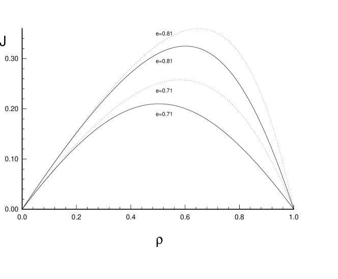
Figure 1: The current versus the density for different values of $e$ in backward updating. Continuous lines refer to $P_{1}(v)$ and dotted lines refer to $P_{2}(v)$.

Remark: Total current $J_{\leftarrow}$ and total density $\rho_{\leftarrow}$ are in general functions of three control parameters $e$, $\alpha$ and $m$. Recalling that $e$ is the average hopping probabilty , $\alpha$ is the total rate of injection and $m$ determines the shape of hopping distribution function. Equation (70) implies that only two parameters are independent. There is a one-to-one correspondence between the two dimensional parameter space defined by the surface (70) and the current-density space. $J_{\leftarrow}$ versus $\rho_{\leftarrow}$ in fig (1) corresponds to ntersection of planes $e=$ constant , with the surface defined by (70). We can instead look at the intersection of $\alpha=$ constant planes with the surface and find the corresponding curves in $J_{\leftarrow}-\rho_{\leftarrow}$ plane. This is done by eliminating $e$ between equations (72) and (73). Figure (2) shows these diagrams for some values of $\alpha$.

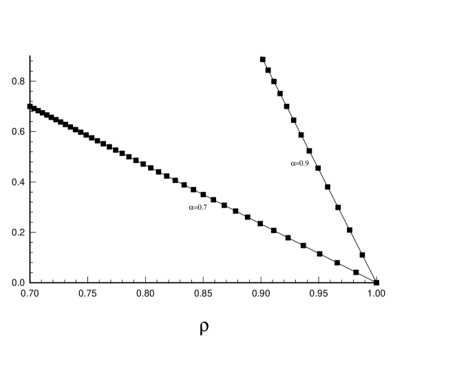
Figure 2: The current versus the density for different values of $\alpha$ in backward updating. Continuous lines refer to $P_{1}(v)$ and filled squares refer to $P_{2}(v)$.

Finally we consider the curves of constant $m$ in $J_{\leftarrow}-\rho_{\leftarrow}$ plane. To obtain these curves, one should write $J_{\leftarrow}$ and $\rho_{\leftarrow}$ in terms of $\alpha$ and $m$ as follows

$$J_{\leftarrow}(\alpha,m)={{\alpha(\alpha+m+1)}\over{(\alpha+m+1)(1-\alpha)+\alpha(m+2)(1+{{\alpha}\over m})}}$$ (74)

$$\rho_{\leftarrow}(\alpha,m)={{\alpha(m+2)(1+{{\alpha}\over m})}\over{(\alpha+m+1)(1-\alpha)+\alpha(m+2)(1+{{\alpha}\over m})}}$$ (75)

Eliminating $\alpha$ between $\rho_{\leftarrow}(\alpha,m)$ and $J_{\leftarrow}(\alpha,m)$ would give us the current-density diagrams for a fixed value of $m$. Figure (3) shows these diagrams for some values of $m$. As can be seen, the current does not vanish at $\rho_{\leftarrow}=1$. This can be explained by noticing that although at $\rho_{\leftarrow}=1$, the chain is completely filled, still we have current via exchange processes. At $\rho_{\leftarrow}=1$, the more decreasing $m$, the more $J_{\leftarrow}$ approaches to zero.

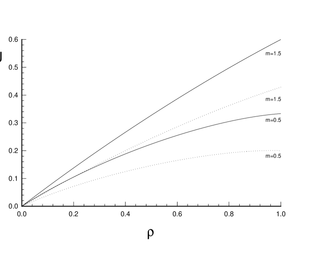
Figure 3: The current versus the density for different values of $m$ in backward updating. Continuous lines refer to $P_{1}(v)$ and dotted lines refer to $P_{2}(v)$.

Using (72) and (74), we can also look at the behaviour of current itself as a function of control parameters. In figures (4) and (5), we show the dependence of $J_{\leftarrow}$ on $\alpha$ ,$e$ for some fixed values of $e$ and $\alpha$. Note that for each $\alpha$, there is a lower limit of $e$ which can be obtained through equation (70).

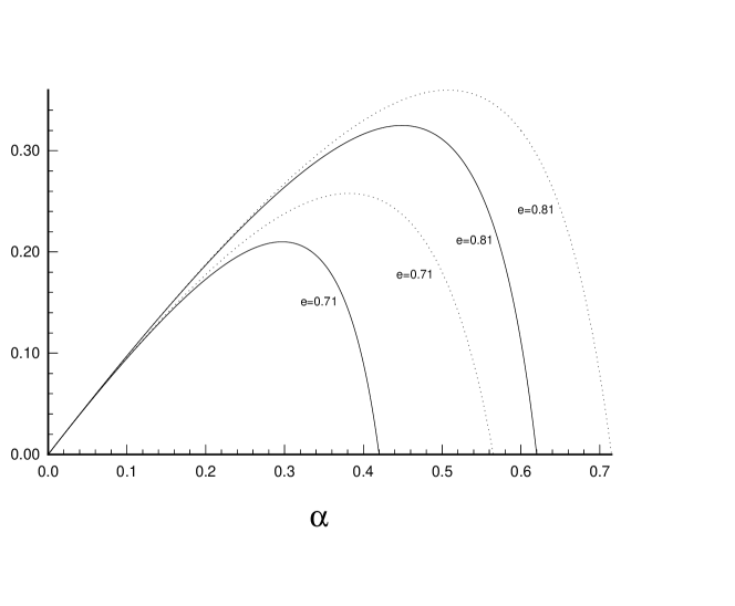
Figure 4: The current versus the arrival probability of particles for different values of $e$ in backward updating. Continuous lines refer to $P_{1}(v)$ and dotted lines refer to $P_{2}(v)$.

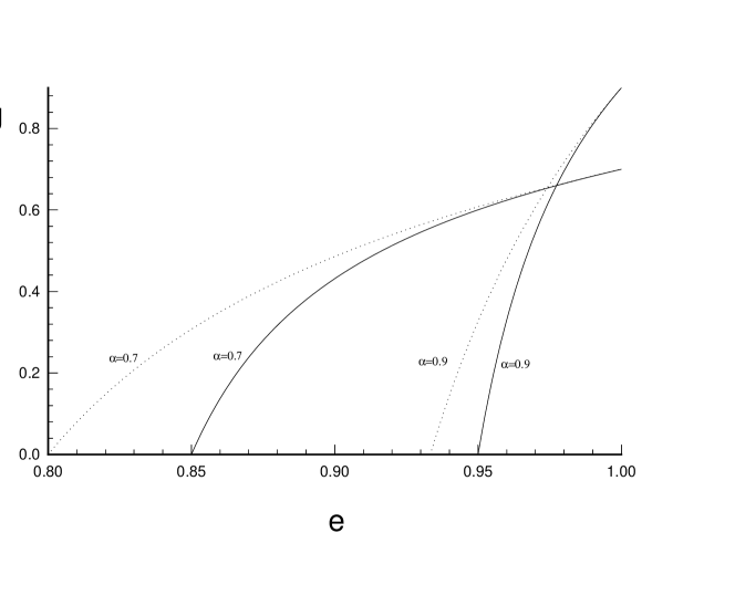
Figure 5: The current versus the total probability of hopping for different values of $\alpha$ in backward updating. Continuous lines refer to $P_{1}(v)$ and dotted lines refer to $P_{2}(v)$.

Our second choice of velocity distribution function is the following

$$P_{2}(v)={{(m+1)(m+2)}\over{(1-\alpha)^{m+2}}}(v-\alpha)^{m}(1-v)\ \ \ m\geq 0$$ (76)

It vanishes at $v=\alpha$ , $v=1$ and has a maximum at $v_{max}={{m+\alpha}\over{m+1}}$. If $m$ increases, $v_{max}$ approaches to one and if $m$ decreases to zero , it approaches to $\alpha$. Inserting $P_{2}(v)$ into (39) we arrive at

$$m={{3e-2\alpha-1}\over{1-e}}$$ (77)

using (67),(68) and (77), we express $J_{\leftarrow}$ and $\rho_{\leftarrow}$ in terms of $e$, $\alpha$ and $\alpha$, $m$

$$J_{\leftarrow}(\alpha,e)={{e\alpha(2\alpha+1-3e)}\over{e(1-\alpha)(2\alpha-3e+1)+\alpha(2\alpha e-3e+1)}}$$ (78)

$$\rho_{\leftarrow}(\alpha,e)={{\alpha(2\alpha e+1-3e)}\over{e(1-\alpha)(2\alpha-3e+1)+\alpha(2\alpha e-3e+1)}}$$ (79)

$$J_{\leftarrow}(\alpha,m)={{\alpha(2\alpha+m+1)}\over{(1-\alpha)(2\alpha+m+1)+\alpha(m+3)({{2\alpha}\over m}+1)}}$$ (80)

$$\rho_{\leftarrow}(\alpha,m)={{\alpha(m+3)({{2\alpha}\over m}+1)}\over{(1-\alpha)(2\alpha+m+1)+\alpha(m+3)({{2\alpha}\over m}+1)}}$$ (81)

We now eliminate $\alpha$ between $J_{\leftarrow}(\alpha,e)$ and $\rho_{\leftarrow}(\alpha,e)$ which leads to current-density diagrams for fixed values of $e$. Dotted lines in fig (1) shows these diagrams for the same values of $e$ .
Similar to $P_{1}(v)$, we can consider the current-density diagrams corresponding to constant $\alpha$ and $m$. These diagrams are shown by dotted lines in figures (2) and (3) respectively. Dependence of $J_{\leftarrow}$ on $\alpha$ and $e$ for $P_{2}(v)$ are also shown in figures (4) and (5) by dotted lines. Note that in figure (5), the curves obtained from $P_{1}(v)$ asymptotically approach to those of $P_{2}(v)$.
Here, we would like to reveal a feature of the infinite species limit which is somehow reminiscent of Bose-Einestein condensation [19]. Equation (68) implies that the density of particles with speed $v$ is proportional to ${vP(v)\over{v-\alpha}}$. Taking (69,76) for $P(v)$ we have

$$\rho(v)\sim v(v-\alpha)^{m-1}$$ (82)

Recalling that $\alpha$ is the minimum speed of particles, equation (82) shows two different kinds of behaviour depending on whether $m>1$ or $m<1$.

I) If $m-1>0$ then $\rho(v)\rightarrow 0$ for $v\rightarrow\alpha$

which means that density of low speed particles is small, i.e. most of the particles move with rather high speed.

II) If $m-1<0$ then $\rho(v)\rightarrow\infty$ for $v\rightarrow\alpha$.

In contrast to the case I, here the density of low-speed particles are large and most of the particles move with low speed , which can be interpreted as appearing of the traffic jammed phase.

5 ${\bf{p}}$-Spesies ASEP with Forward Updating

5.1 Formulation

As stated in the introduction and section (2), instead of right to left (backward) updating, one can change the direction of updating and starts from the first site of the chain (forward updating) and updates from the left to the right in the same manner of backward updating. Most of the steps are similar to backward updating and we only write the results. The transfer matrix takes the following form

$$T_{\rightarrow}=R_{L}T_{L-1,L}...T_{1,2}L_{1}$$ (83)

All the matrices are the same as in (17,18,19). The MPS for the steady state is written as [23]

$$|P_{s}>_{\rightarrow}=<<W|\hat{A}\otimes\hat{A}\otimes...\otimes\hat{A}|V>>$$ (84)

Taking $A$ and $\hat{A}$ to satisfy the same algebra (21-23), makes $|P_{s}>_{\rightarrow}$ to be a stationary state i.e. $T_{\rightarrow}|P_{s}>_{\rightarrow}=|P_{s}>_{\rightarrow}$. Here at first site $i=1$ a ”defect” $A$ is created, then transmited forward until it reaches the last site $i=L$ where it disappears. Next we consider formulas for the currents and densities. Here the situation is quite different and the difference between forward and backward updating reveals itself. The definition of currents reads from (49-51) and $T_{\leftarrow}$ is replaced with (83). The mean current of $i$-type particles through site $k$ is found to be

$$<J_{k-1,k}^{(i)}>_{\rightarrow}={{<W|\hat{C}^{k-2}J^{(i)}\hat{C}^{L-k}|V>}\over{<W|\hat{C}^{L}|V>}}$$ (85)

Where $J^{(i)}$ is the same as equation (53), and $\hat{C}=\hat{E}+\sum_{i=1}^{p}{\hat{D}_{i}}$. We again demand that $\hat{E}$ and ${\hat{D}_{i}}$ satisfy equation (33,34) which in turn let us revisit equation (42-45) and thus we have

$$J^{(i)}=d_{i}C$$ (86)

$$\hat{C}=C$$ (87)

Putting (86,87) in (85) yields

$$<J^{(i)}>_{\rightarrow}=d_{i}{{<W|C^{L-2}|V>}\over{<W|{C}^{L}|V>}}$$ (88)

Also one can write the mean density of $i$-type particles at site $k$

$$<n_{k}^{(i)}>_{\rightarrow}={<W|{C}^{k-1}(D_{i}-v_{i})C^{L-k}|V>\over<W|C^{L}|V>}$$ (89)

5.2 One dimensional representation and infinite number of species limit in forward updating

Again scaling all $D_{i}$’s by a ${1\over p}$ factor, we now take ${D_{i}\over p}$ and $E$ to be c-numbers. Similar to backward update, they are ${{\cal{D}}_{i}\over p}$ and ${\cal{E}}$ respectively and the equations (58-61) remain the same. In one dimensional representation, the densities and the currents of $i$-type particles are all site independent and are respectively given by

$$\rho_{\rightarrow}(\alpha,i)={({{\cal{D}}_{i}\over p}-{v_{i}\over p})\over{e({1\over\alpha}-1)+{{\cal{D}}\over p}}}\ \ \ ,\ \ J_{\rightarrow}(\alpha,i)={{v_{i}\over p}\over{e({1\over\alpha}-1)+{{\cal{D}}\over p}}}$$ (90)

Comparing the above equations with their counterparts in backward updating, we see that currents do not change but forward density undergoes the following modification

$$J_{\rightarrow}(\alpha,i)=J_{\leftarrow}(\alpha,i)=J(\alpha,i)\ \ ,\ \ \rho_{\rightarrow}(\alpha,i)=\rho_{\leftarrow}(\alpha,i)-J(\alpha,i)$$ (91)

The above relations reveals the difference between forward and backward updating. Similar relation between backward and forward densities is seen in [23]. We again define the total density and current by summing over densities and currents of all kind of species

$$J_{\rightarrow}(\alpha)=J_{\leftarrow}(\alpha)={e\over{e({1\over\alpha}-1)+{{\cal{D}}\over p}}}\ \ ,\ \ \rho_{\rightarrow}(\alpha)=\rho_{\leftarrow}(\alpha)-J(\alpha)$$ (92)

Now we take the limit of $p\rightarrow\infty$. Adopting the same distribution functions $P_{1}(v)$ , $P_{2}(v)$ and using (92), one easily can obtain $J_{\rightarrow}$ and $\rho_{\rightarrow}$ as functions of $e$ , $\alpha$ and $m$ , both for $P_{1}(v)$ and $P_{2}(v)$. Similar to the backward scheme, the corresponding current-density diagrams can be obtained by eliminating one of the control parameters. These diagrams are shown in figures (6) to (8).

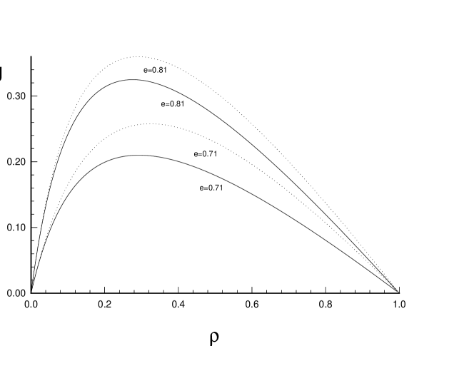
Figure 6: The current versus the density for different values of $e$ in forward updating. Continuous lines refer to $P_{1}(v)$ and dotted lines refer to $P_{2}(v)$.

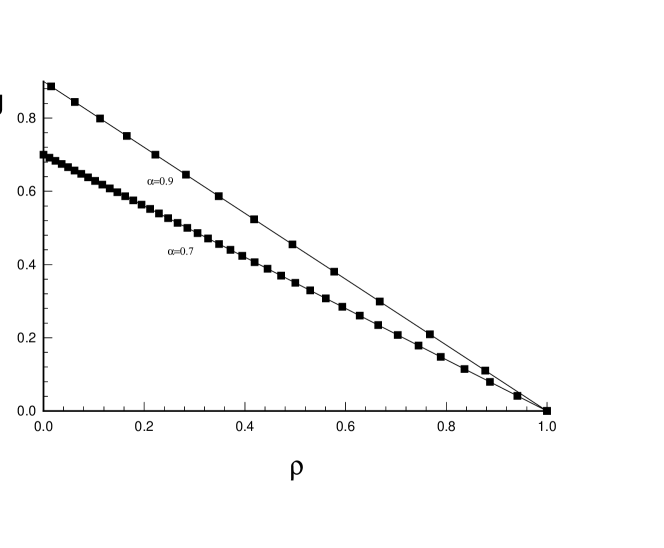
Figure 7: The current versus the density for different values of $\alpha$ in forward updating. Continuous lines refer to $P_{1}(v)$ and filled squares refer to $P_{2}(v)$.

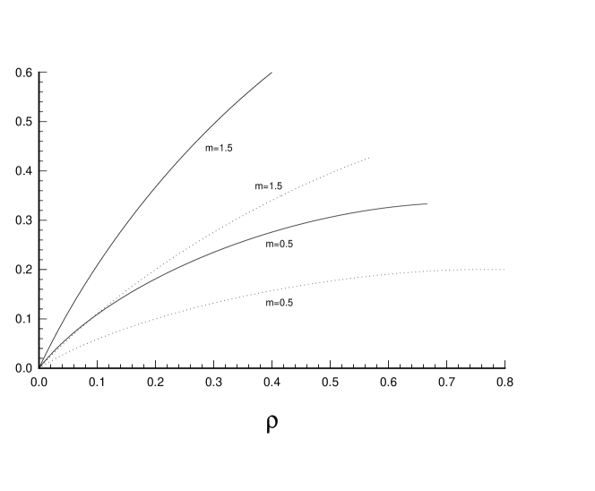
Figure 8: The current versus the density for different values of $m$ in forward updating. Continuous lines refer to $P_{1}(v)$ and dotted lines refer to $P_{2}(v)$.

Remark:
Surprisingly as can be seen in fig(7), when $\rho_{\rightarrow}$ goes to zero, the value of $J_{\rightarrow}$ does not vanish. This is in contrast to other’s results and is an exclusive effect appearing only in forward updating which can be explained by noting that, when the lattice is completely empty, in first site a particle is injected with the probability $\alpha$ and according to the multiplicative nature of the transition matrix is transfered through the lattice, hence one has a non-zero current.
In general, the value of $J_{\rightarrow}$ at $\rho_{\rightarrow}=0$ is equal to $\alpha$ and this point refers to the point $(m=\infty,e=1,\alpha)$ in parameter space.

We would like to end this section with some remarks on sub-parallel updating scheme. In fact as stated in section 1, there are few exact results in parallel updating. The root of this difficulty is the non-local nature of transfer matrix which in contrast to the ordered sequential updating, can not be written as a product of local transfer matrices. A simpler case is to consider a sub-parallel updating scheme. In this scheme, one proceeds with two half time-steps. In the first half, one updates the first site, last site and all pairs $(\tau_{i},\tau_{i+1})$ with an even $i$ ($L$ is taken to be even). Then in the second half time-step, one updates all pairs $(\tau_{i},\tau_{i+1})$ with $i$ odd. So the transfer matrix is

$$T_{sp}=T_{sp}^{(2)}T_{sp}^{(1)}$$ (93)

with

$$T_{sp}^{(1)}=L_{1}T_{2,3}T_{4,5}\cdots T_{L-2,L-1}R_{L}$$ (94)

$$T_{sp}^{(2)}=T_{1,2}T_{3,4}\cdots T_{L-1,L}$$ (95)

Defining MPS for sub-parallel updating as follows [25]

$$|P_{s}>_{sp}=<<W|\hat{A}\otimes A\otimes\hat{A}\otimes\cdots\hat{A}\otimes A|V>>$$ (96)

It can be verified that $T_{sp}|P_{s}>_{sp}=|P_{s}>_{sp}$ provided that equations (21-23) are satisfied.

It is shown in [32] that sub-parallel and ordered sequential updating schemes are intimately related to each other. It is proved that in general the following correspondence exists

$$<n_{k}^{(i)}>_{sp}=\cases{<n_{k}^{(i)}>_{\rightarrow}&$k$ odd\cr<n_{k}^{(i)}>_{\leftarrow}&$k$ even\cr}$$ (97)

$$<n_{k}^{(i)}n_{l}^{(j)}>_{sp}=\cases{<n_{k}^{(i)}n_{l}^{(j)}>_{\rightarrow}&$k$ , $l$ odd\cr<n_{k}^{(i)}n_{l}^{(j)}>_{\leftarrow}&$k$ , $l$ even\cr}$$ (98)

where $k$ and $l$ refer to the lattice sites and $i$ and $j$ refer to the state of the site. Using this general correspondence, we obtain the density profile of $p$-species ASEP under sub-parallel updating ( one dimensional representation )

$$<n_{k}^{(i)}>_{sp}={{{\cal{D}}_{i}\over p}\over e({1\over\alpha}-1)+{{\cal{D}}\over p}}\ \ \ \ k=even$$ (99)

$$<n_{k}^{(i)}>_{sp}={{{\cal{D}}_{i}\over p}-{v_{i}\over p}\over e({1\over\alpha}-1)+{{\cal{D}}\over p}}\ \ \ \ k=odd$$ (100)

6 ${\bf p}$-Species ASEP with Ordered Updating on a Ring

In this section we consider the $p$-species ASEP on a closed ring of $N$ sites. We work in a canonical ensemble in which the number of each species $(i)$ is fixed to be $m_{i}$ and we take the total number of particles to be $M$ i.e. $\sum_{i=1}^{p}m_{i}=M$ .
The periodic system can be described by a one dimensional representation of the bulk algebra (24-28). In this case the bulk algebra reduces to the following equations

$$(1-v_{i})d_{i}\hat{e}=\hat{d}_{i}e$$ (101)

$$({{1-v_{j}}\over{1-v_{i}}})d_{j}\hat{d_{i}}=\hat{d_{j}}d_{i}$$ (102)

The above equations yield

$$\hat{d_{j}}={{\hat{e}}\over{e}}(1-v_{j})d_{j}$$ (103)

Here $d_{i}$ and $\hat{d_{i}}$, correspond to one dimensional representations of $D_{i}$ and $\hat{D_{i}}$ (not to be confused with those introduced in (34)). Using (53) and (57) we obtain the following forms for the density and the current of $i$-type particles :

$$\rho_{\leftarrow}^{(i)}={{d_{i}}\over{e+\sum_{i}d_{i}}},\ \ \ J_{\leftarrow}^{(i)}=\hat{e}(v_{i}d_{i}+{1\over{e}}[v_{i}d_{i}\sum_{j}d_{j}-d_{i}\sum_{j}d_{j}v_{j}])$$ (104)

Summing over $i$, we obtain the total current and density

$$\rho_{\leftarrow}={\sum_{i}d_{i}\over{e+\sum_{i}d_{i}}}\ \ ,\ \ J_{\leftarrow}=\hat{e}\sum_{i}{v_{i}d_{i}}$$ (105)

Defining the population averaged velocity ${<v>}$ as follows

$$<v>={{\sum_{i}m_{i}v_{i}}\over{\sum_{i}m_{i}}}$$ (106)

and rescaling the $d_{i}$’s and $e$ so that

$$e+\sum_{i}d_{i}=\hat{e}+\sum_{i}\hat{d_{i}}=1$$ (107)

we arrive at

$$J_{\leftarrow}={{{<v>}\rho_{\leftarrow}(1-\rho_{\leftarrow})}\over{1-{<v>}\rho_{\leftarrow}}}$$ (108)

which is the current-density relation of $p$-species ASEP on a ring with backward updating. Comparing it with the usual ASEP on ring with backward updating in [23] , we see that they both have the same form. In $p$ species model, ${<v>}$ plays the role of hopping probability in usual ASEP. Fig (9) shows $J_{\leftarrow}$ versus $\rho_{\leftarrow}$ for different values of ${<v>}$.

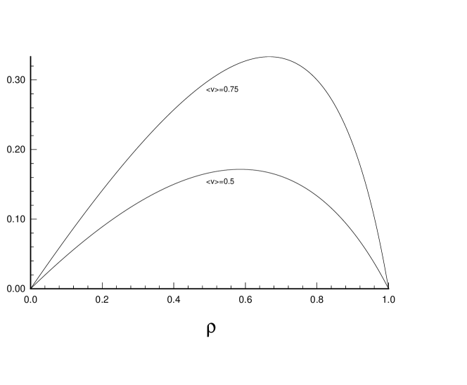
Figure 9: The current versus the density for different values of $<v>$ in backward updating.

The maximum current occurs at

$$\rho_{\leftarrow}^{max}({<v>})={1-(1-({<v>})^{1\over 2})\over{<v>}}\geq{1\over 2}$$ (109)

We now consider the forward updating. Note that since we don’t have particle-hole symmetry, the current-density relation in forward updating can not be obtain from the one in backward updating and should be considered seperately. In forward updating we have

$$\rho_{\rightarrow}^{(i)}={\hat{d_{i}}\over\hat{e}+\sum_{i}\hat{d_{i}}}\ \ ,\ \ J_{\leftarrow}^{(i)}=J_{\rightarrow}^{(i)}$$ (110)

Using (101-103) and (107), after straightforward calculations, we arrive at

$$J_{\rightarrow}={(1-\rho_{\rightarrow})\rho_{\rightarrow}<{v\over 1-v}>\over 1+\rho_{\rightarrow}<{v\over 1-v}>}$$ (111)

where

$$<{v\over 1-v}>={\sum_{i}{v_{i}\over 1-v_{i}}m_{i}\over\sum_{i}m_{i}}$$ (112)

If we now take $p=1$ , $<{v\over 1-v}>$ will reduce to $v_{1}\over 1-v_{1}$ and (111) takes the following form

$$J_{\rightarrow}={{v_{1}\rho_{\rightarrow}(1-\rho_{\rightarrow})}\over{1-{v_{1}}\rho_{\rightarrow}}}$$ (113)

and the particle-hole symmetry is recovered [23] i.e. (113) is obtained from (108) by changing $\rho_{\leftarrow}$ to $1-\rho_{\rightarrow}$.

Fig(10) shows $J_{\rightarrow}$ versus $\rho_{\rightarrow}$ for different values of $<{v\over 1-v}>$.

The maximum of $J_{\rightarrow}$ has moved to the left. This maximum occurs at

$$\rho_{\rightarrow}^{max}(<{v\over 1-v}>)={1\over<{v\over 1-v}>}[(1+<{v\over 1-v}>)^{1\over 2}-1]\leq{1\over 2}$$ (114)

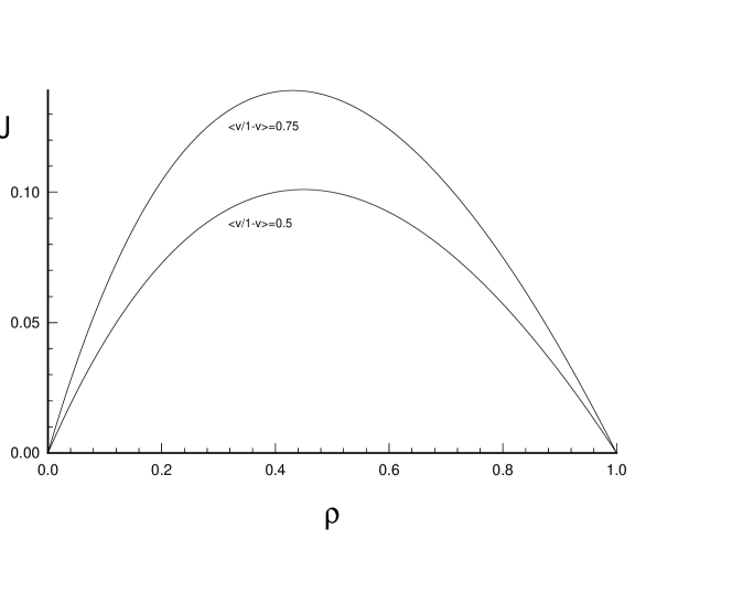
Figure 10: The current versus the density for different values of $<{v\over{1-v}}>$ in backward updating.

7 Comparison and Concluding Remarks

Here we compare our results with those of [20] and specify the similarities and differences between ordered and random sequential updating procedures. Both procedures are described by a similar quadratic algebra. In random update, time should be so rescaled such that the average hopping rate equals one. On the contrary in ordered updating the average hopping probability $e$ remains as a free parameter. This is one of the main differences between two updating schemes. In both schemes, injection rate (probability) of an $i$-type particle ($\alpha_{i}$) is proportional to its hopping rate (probability) $v_{i}$.
When considering infinite species limit, one can investigate the characteristics of both schemes with a limited number of control parameters. As long as analytical calculations are concerned, these control parameters are $\alpha$ , $e$ and $m$ in ordered schemes and $\alpha$, $m$ and $\lambda$ in random scheme where $m$, $\lambda$ determine the shape of distribution function [20]. One of the advantages of ordered scheme is the appearance of the more physical parameter $e$ in control parameters, which is absent in random scheme.
In this paper, we made a more complete investigation of the current- density and current diagrams for different regions of parameter space.
We also evaluated the dependence of the current on the density for fixed values of $\alpha$ in random scheme. The corresponding diagram is quite similar to ours in figure (2) but the values of current and minimum allowed value of the density are different.
All the result of this paper and [20] have been obtained in a restricted region of parameters space ($\alpha_{i},\beta_{i},v_{i}$) where mean field approximation becomes exact. It would be a highly nontrivial task to investigate the physical properties of the hole regions of parameter space either by infinite dimensional representations or by the explicit use of quadratic algebra. Consideration of $p$-species ASEP under fully parallel updating is another interesting subject which is under study.

Acknowledgement:
We would like to thank V.Karimipour for his valuable comments and discussions. We also appreciate M.Abolhasani, A.Langari and J.Davoodi for their useful helps.

References

- [1] V. Privman (Ed.), Nonequilibrium Statistical Mechanics in One Dimension (Cambridge University Press, 1997)
- [2] B. Schmittmann and R.K.P. Zia, Statistical Mechanics of Driven Diffusive Systems (Academic Press, 1995)
- [3] H. Spohn, Large Scale Dynamics of Interacting Particles (Springer, 1991)
- [4] G.M. Schütz, Integrable stochastic many body systems (Jülich preprint,Jül-3555)
- [5] J. Krug, Boundary induced phase transition in driven diffusive systems, Phys. Rev. Lett. 67, 1882 (1991)
- [6] M.R. Evans, D.P. Foster, C. Godrèche and D. Mukamel, Asymmetric exclusion model with two species: Spontaneous symmetry breaking, J. Stat. Phys. 80, 69 (1995)
- [7] P.F. Arndt, T. Heinzel and V. Rittenberg, Spontaneous breaking of translational invariance and spatial condensation in stationary state on a ring, cond-mat/9809123
- [8] D. Kandel, G. Gershinsky, D. Mukamel and B. Derrida, Phase transition induced by a defect in growing interface model, Physica Scrai pta T49 , 622 (1993)
- [9] S.A. Janowsky, J.L. Lebowitz, Finite size effects and shock fluctuations in an asymmetric simple exclusion process, Phys. Rev. A45, 618 (1992)
- [10] A.B. Kolomeisky, Asymmetric simple exclusion model with local inhomogeneity, J. Phys. A: Math Gen. 31, 1153 (1998)
- [11] K. Mallick, Shocks in the asymmetry exclusion model with an impurity, J. Phys. A: Math Gen. 29, 5375 (1996)
- [12] H-W. Lee, V. Popkov and D. Kim, Two way traffic flow: Exactly solvable model of traffic jam, J. Phys. A: Math Gen. ,30, 8497 (1997)
- [13] B. Derrida, An exactly soluble non-equilibrium system: The asymmetric simple exclusion model, Phys. Rep. 301, 65 (1998)
- [14] K. Nagel and M. Schreckenberg, J. Phys. I France 2, 2221 (1992)
- [15] M. Schreckenberg, A. Schadschneider, K. Nagel and N. Ito, Discrete stochastic models for traffic flow, Phys. Rev. E51 2939 (1995)
- [16] Proceedings of the workshop on ”Traffic and granular flow 97 ”, (Springer, 1998)
- [17] B. Derrida, M.R. Evans, V. Hakim and V. Pasquier, Exact solution of a 1d asymmetric exclusion model using a matrix formulation, J. Phys. A: Math Gen. 26, 1493 (1993)
- [18] B. Derrida, S.A. Janowsky, J.L. Lebowitz and E.R. Speers, Exact solution of the totally ASEP: Shock profiles, J. Stat. Phys. 73 , 813 (1993)
- [19] M.R. Evans, Phase transitions in disordered exclusion models: Bose condensation in traffic flow Europhys. Lett. 36, 1493 (1996)
- [20] V. Karimipour, A multi-species ASEP and its relation to traffic flow, cond-mat/9808220, to appear in Phys. Rev. E
- [21] V. Karimipour, A multi-species ASEP, Steady state and correlation functions on a periodic lattice, preprint, cond-mat/9809193
- [22] F.C. Alcaraz, M. Droz, M. Henkel and V. Rittenberg, Reaction-Diffusion process, critical dynamics and quantum chains, Ann.Physics. 230, 250 (1994)
- [23] N. Rajewsky, L. Santen, A. Schadschneider and M. Schreckenberg, The asymmetric exclusion process: Comparison of update procedures, J. Stat. Phys. 92, 151 (1998)
- [24] G.M. Schütz, Time-dependent correlation functions in a one-dimensional asymmetric exclusion process, Phys. Rev. E47, 4265 (1993)
- [25] H. Hinrichsen, Matrix product ground states for exclusion processes with parallel dynamics, J. Phys. A: Math Gen. 29, 3659 (1996)
- [26] H. Hinrichsen and S. Sandow, Deterministic exclusion process with a stochastic defect: Matrix product ground states, J. Phys. A: Math Gen. 30, 2745 (1997)
- [27] N. Rajewsky, A. Schadschneider and M. Schreckenberg, The asymmetric exclusion model with sequential update, J. Phys. A: Math Gen. 29, L305 (1996)
- [28] A. Honecker and I. Peschel, Matrix-product states for a one-dimensional lattice gas with parallel dynamics, J. Stat. Phys. 88, 319 (1997)
- [29] M.R. Evans, Exactly steady state of disordered hopping particles with parallel and ordered sequential dynamics, J. Phys. A: Math Gen. 30, 5669 (1997)
- [30] M.R. Evans, N. Rajewsky and E.R. Speer, Exact solution of a cellular automaton for traffic, cond-mat/9810306
- [31] K. Krebs and S. Sandow, Matrix product eigenstates for one-dimensional stochastic models and quantum spin chains, J. Phys. A: Math Gen. 30, 3165 (1997)
- [32] N. Rajewsky and M. Schreckenberg, Exact results for one dimensional stochastic cellular automata for different types of updates, Physica A245, 139 (1997)
- [33] N. Rajewsky, A. Schadschneider and M. Schreckenberg, The asymmetric exclusion model with sequential update, J. Phys. A: Math Gen. 29, L305 (1996)