[

Andreev Reflection and Spin Injection into $s-$ and $d-$wave Superconductors

Abstract

We study the effect of spin injection into $s-$ and $d-$wave superconductors, with an emphasis on the interplay between boundary and bulk spin transport properties. The quantities of interest include the amount of non-equilibrium magnetization ($m$), as well as the induced spin-dependent current ($I_{s}$) and boundary voltage ($V_{s}$). In general, the Andreev reflection makes each of the three quantities depend on a different combination of the boundary and bulk contributions. The situation simplifies either for half-metallic ferromagnets or in the strong barrier limit, where both $V_{s}$ and $m$ depend solely on the bulk spin transport/relaxation properties. The implications of our results for the on-going spin injection experiments in high $T_{c}$ cuprates are discussed.

]

A number of spin-injection experiments have recently been carried out for the high $T_{c}$ cuprates[1, 2, 3, 4, 5]. These experiments are of interest for a variety of reasons. In particular, they in principle allow us to extract the bulk spin transport properties of the high $T_{c}$ cuprates. In the normal state, such spin transport properties have been proposed as a probe of spin-charge separation[6, 7]. In the superconducting state, they can provide important clues to the nature of the quasiparticles. In addition, the anisotropy of the spin transport properties should shed new light on the nature of the $c-$axis transport. Finally, spin-injection into superconductors also provides a setting to study the phenomenon of spatial separation of charge and spin currents[8, 9].

For the purpose of extracting the bulk spin transport properties, it is essential that their contributions to the measured physical quantities are separated from those of the boundary transport processes. The boundary of interest here is formed between the high $T_{c}$ cuprates and ferromagnetic metals. One transport process through such a boundary is the Andreev reflection[10], which carries pair-current into the superconductor. The novel features of the Andreev reflection involving a ferromagnet have recently been addressed[11, 12, 13]. Another boundary process is the single-particle transport. While the charge transport involves both processes, the spin transport proceeds through the single-particle process only. The interplay between the two processes is therefore expected to play an important role in the spin injection experiments. The consequences of such an interplay are explored in this paper. The $s-$wave case is simpler, which we will address first. (This part of our analysis is also relevant to the spin injection experiments in the non-cuprate superconductors[14, 15].) We will then extend our analysis to the $d-$wave case.

Several physical quantities are of interest in spin injection experiments. One is the amount of non-equilibrium magnetization ($m$) injected into the superconductor. The others include the spin-dependent current ($I_{s}$) and boundary voltage ($V_{s}$) induced by the injected magnetization. We will show below that, in general these quantities reflect very different combinations of the bulk spin transport and interface transport contributions.

The relevant experimental setups are illustrated in Fig. 1. Fig. 1a) is representative of those used in the on-going spin-injection experiments in the high $T_{c}$ cuprates[1, 2, 3, 4]. An injection current ($I$, per unit area) from a ferromagnetic metal (FM1) to the superconductor (S) is applied, and the critical current of the superconductor is then measured. The suppression of the critical current, $\Delta J_{c}\equiv(J_{c}(I=0)-J_{c}(I))/J_{c}(I=0)$, is expected to be a measure of the amount of injected magnetization ($m$). Fig. 1b) illustrates the spin-injection-detection setup of Johnson and Silsbee[16, 5]. Here a superconductor (S) is in contact with two itinerant ferromagnets, FM1 and FM2. The magnetization of FM1 is either parallel ($\sigma=\uparrow$) or antiparallel ($\sigma=\downarrow$) to that of FM2. For a given $\sigma$, $I_{\sigma}$ is the induced current across the S-FM2 interface in a closed circuit. Likewise, $V_{\sigma}$ is the induced boundary voltage ($V_{\sigma}$) in an open circuit. The spin-dependent current and boundary voltage are defined as $I_{s}=I_{\uparrow}-I_{\downarrow}$ and $V_{s}=V_{\uparrow}-V_{\downarrow}$, respectively.

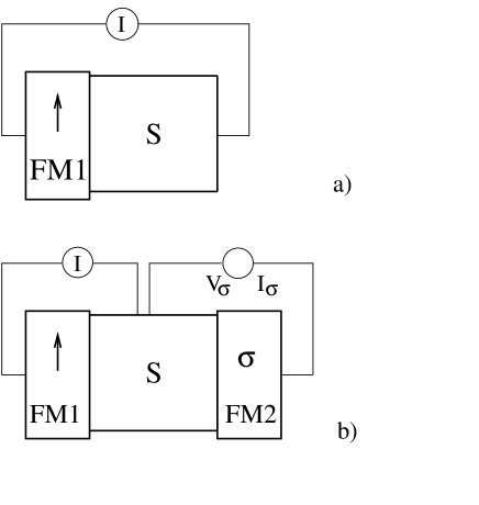
FIG. 1.: a) A spin injection setup involving a ferromagnetic metal (FM1) and a superconductor (S). b) A spin-injection-detection setup involving a superconductor (S) and two ferromagnetic metals (FM1 and FM2).

To highlight the interplay between the boundary and bulk transport processes, we will make a number of simplifying assumptions. The superconductor (S) is assumed to be a BCS superconductor, with either an $s-$wave or a $d_{x^{2}-y^{2}}-$wave order parameter. The ferromagnetic metal will be simply modeled by an exchange energy $h$[11, 17]. The Hamiltonians for FM1 and FM2 are, ${\cal H}_{1}=\sum_{k,\tau}(\epsilon_{k}-h\tau)c_{k,\tau}^{\dagger}c_{k,\tau}$ and ${\cal H}_{2}=\sum_{k,\tau}(\epsilon_{k}-h\tau\sigma)c_{k,\tau}^{\dagger}c_{k,\tau}$, respectively. The unshifted energy dispersions for both ferromagnets are assumed to be $\epsilon_{k}={\hbar}^{2}k^{2}/2m$, as is the normal state energy dispersion for the superconductor. In addition, the Fermi wavevectors of the superconductor and the ferromagnets in the absence of polarization are assumed to be equal to $k_{f}$. For FM1, this implies $k_{f\tau}=k_{f}t_{\tau}$ and a Fermi velocity $v_{f\tau}=v_{f}t_{\tau}$ where

$$t_{\tau}\equiv\sqrt{1+\tau h/\epsilon_{f}}$$ (1)

For FM2, $k_{f\tau}=k_{f}t_{\sigma\tau}$ and $v_{f\tau}=v_{f}t_{\sigma\tau}$.

We introduce $m(x)$ to denote the steady state spin magnetization density in the superconductor. Since $m(x)$ is entirely carried by the quasiparticles, it satisfies

$$-D_{s}{\partial^{2}m/\partial x^{2}}=-{{m(x)}/T_{1}}$$ (2)

where $T_{1}$ is the longitudinal spin relaxation time and $D_{s}$ is the spin diffusion constant.

We now specify the boundary conditions. For the setup of Fig. 1a), $x=0$ and $x=d$ correspond to the FM1-S interace and the open end of S, respectively. For Fig. 1b), they instead describe the FM1-S and S-FM2 interfaces, respectively. At $x=0$,

$$-D_{s}\partial m/\partial x|_{x=0}=I_{spin}$$ (3)

For the setup of Fig. 1a), and to the leading order in Fig. 1b) as well, the boundary condition at $x=d$ is

$$-D_{s}\partial m/\partial x|_{x=d}=0$$ (4)

The crucial question then is, what is the spin-current $I_{spin}$ for a fixed injection electrical-current $I$. At the FM1-S boundary the electrical current is the sum of a pair current ($I_{pair}$), carried through Andreev reflection, and a single-particle current ($I_{sp}$),

$$I=I_{pair}+I_{sp}$$ (5)

The spin current, on the other hand, has no contribution from the Andreev process given that the Cooper pairs are spin singlets. We then expect,

$$I_{spin}=\eta\mu_{B}I_{sp}/e$$ (6)

where $\eta$ is the single-particle current polarization, which itself also needs to be determined. In the following, we first calculate the three currents, $I_{pair}$, $I_{sp}$, and $I_{spin}$, for a given voltage, $V$, across the FM1-S barrier. The latter can then be expressed in terms of $I$, through Eq. (5), leading to an expression for $I_{spin}$ as a function of $I$.

For a fixed $V$, the values of the three currents depend on the nature of the interface. Here, we model this interface by a delta-function potential, ${\cal H}_{interface}={\cal V}\delta(x)$. The Bogoliubov-deGennes equation[18] is,

$$\left(\begin{array}[]{ll}{\cal H}_{0}-h\tau{}{}{}{}{}{}{}{}{}&\Delta\\ \Delta^{*}{}{}{}{}{}{}{}{}{}&-({\cal H}_{0}+h\tau)\end{array}\right)\left(\begin{array}[]{ll}u_{\tau}\\ v_{\bar{\tau}}\end{array}\right)=E\left(\begin{array}[]{ll}u_{\tau}\\ v_{\bar{\tau}}\end{array}\right)$$ (13)

where ${\cal H}_{0}=p^{2}/2m-\mu+{\cal H}_{interface}$. Here, $h$ and $\Delta$ are non-zero only for $x<0$ and $x>0$, respectively. Inside FM1, the solution is the sum of three plane waves, describing the incident electron of spin $\tau$ and wavevector $\vec{k}_{i\tau}$, the Andreev-reflected hole of spin $\bar{\tau}$, wavevector $\vec{k}_{a\tau}$ and amplitude $a_{\tau}$, and the normally-reflected electron of spin ${\tau}$, wavevector $\vec{k}_{b\tau}$ and amplitude $b_{\tau}$, respectively. Inside the superconductor, the solution is the sum of two plane waves, one without branch-crossing and of wavevector $\vec{k}_{c\tau}$ and amplitude $c_{\tau}$, the other with branch-crossing and of wavevector $\vec{k}_{d\tau}$ and amplitude $d_{\tau}$. The wavevectors are determined by the requirement that, the components parallel to the interface are equal. The amplitudes are then calculated by solving Eq. (13), together with the boundary conditions[18] appropriate to this equation. These amplitudes, in turn, allow us to determine the various currents.

In the linear response regime, the pair, single-particle, and spin currents can be written as $I_{\lambda}/V=\int dE(-\partial f/\partial E)\sum_{\vec{k}\tau}{\cal F}\delta(\xi_{k}^{\tau}-E)v_{k}^{x}i_{\lambda}^{\tau}(E,\vec{k})$. Here, $\xi_{k}^{\tau}=\epsilon_{k}-\epsilon_{f}-h\tau$, $f(E)$ is the Fermi-Dirac distribution function, ${\cal F}$ is a filtering factor which specifies the distribution of incident angles. In addition,

$$i_{pair}^{\tau} =2e^{2}A_{\tau}$$ (14)

$$i_{sp}^{\tau} =e^{2}(C_{\tau}+D_{\tau})$$ (15)

$$i_{spin}^{\tau} ={\mu_{B}}e(C_{\tau}+D_{\tau})\tau$$ (16)

where $C_{\tau}=|c_{\tau}|^{2}(u(k_{c\tau})^{2}-v(k_{c\tau})^{2})v_{f}^{x}/v_{k\tau}^{x}$, $D_{\tau}=|d_{\tau}|^{2}(u(k_{d\tau})^{2}-v(k_{d\tau})^{2})v_{f}^{x}/v_{k\tau}^{x}$, and $A_{\tau}=|a_{\tau}|^{2}v_{k\bar{\tau}}^{x}/v_{k\tau}^{x}$. (Here $k\tau$ labels the wavevectors satisfying $\xi_{k}^{\tau}=E$.)

The potential barrier can be represented in terms of a dimensionless quantity, $z=m{\cal V}/{\hbar}^{2}k_{f}$. In the following, we will focus on the two extreme limits, $z\rightarrow 0$ and $z\rightarrow\infty$. In the latter case we expand in terms of $1/z$. In addition, we will consider only temperatures low compared to the superconducting gap $\Delta$. These cases are sufficient to illustrate the main points of this paper. More general cases will be discussed elsewhere.

$s-$wave, vanishing barrier:   We address first the case of an isotropic $s-$wave superconductor, in the limit of a vanishing barrier, $z=0$. For $k_{B}T\ll\Delta$, we found,

$$I_{pair}/V =g_{0}P_{s,0}$$ (17)

$${I_{sp}/V} =g_{0}S_{s,0}Y_{s,0}(T)$$ (18)

$${I_{spin}/V} =(\mu_{B}/e)g_{0}M_{s,0}Y_{s,0}(T)$$ (19)

Here $g_{0}=N_{0}v_{f}e^{2}$ where $N_{0}$ is the density of states at the unshifted Fermi energy, $P_{s,0}=16\alpha_{pair}{{t_{\uparrow}t_{\downarrow}}/{(t_{\uparrow}t_{\downarrow}+1)^{2}}}$, $S_{s,0}=2\sqrt{2\pi}\alpha_{sp}{{[t_{\uparrow}(t_{\downarrow}^{2}+1)+t_{\downarrow}(t_{\uparrow}^{2}+1)]}/{(t_{\uparrow}t_{\downarrow}+1)^{2}}}$, and $M_{s,0}=2\sqrt{2\pi}\alpha_{spin}{{(t_{\uparrow}-t_{\downarrow})(1-t_{\uparrow}t_{\downarrow})}/{(t_{\uparrow}t_{\downarrow}+1)^{2}}}$. The (polarization-dependent) factors $\alpha_{pair}$, $\alpha_{sp}$, and $\alpha_{spin}$ are of order unity; they describe the averaging over the angle of incident electrons, and are all equal to unity when forward incidence dominates.

Both $I_{sp}$ and $I_{spin}$ have an exponential temperature dependence, as specified by the function $Y_{s,0}(T)=\sqrt{{k_{B}T}/\Delta}e^{-\Delta/k_{B}T}$. This reflects the simple physics that the transport of both the single-particle current and spin current involve the quasiparticles of the superconductor and hence only energies above the superconducting gap.

We are now in a position to determine the non-equilibrium magnetization ($m$) and the induced spin-dependent boundary voltage ($V_{s}$) and current ($I_{s}$) as a function of $I$. Consider first the general case, when the ferromagnet has a less than 100% polarization. For $k_{B}T\ll\Delta$, $I_{pair}$ then dominates the total current in Eq. (5). As a result,

$$I_{spin}/I=(\mu_{B}/e)(M_{s,0}/P_{s,0})Y_{s,0}(T)$$ (20)

Combining Eq. (20) with Eqs. (2, 3, 4), we have,

$${m(x=d)/I}=(\mu_{B}/e)(M_{s,0}/P_{s,0})Y_{s,0}(T){T_{1}\over{\delta_{s}\sinh(d/\delta_{s})}}$$ (21)

where $\delta_{s}=\sqrt{D_{s}T_{1}}$ is the spin-diffusion length of the superconductor.

This magnetization accumulation leads to a drop across the interface of an effective magnetic field[16], $\Delta H=m/\chi$ where $\chi$ is the uniform spin susceptibility of the superconductor. In the spin-injection-detection setup (Fig. 1b), for a closed circuit, this effective field drop will induce a current across the S-FM2 interface. Following a procedure similar to the one leading to Eq. (16), we found

$$I_{\sigma}^{closed}=\sigma g_{0}(\mu_{B}/e)M_{s,0}Y_{s,0}(T)(m/\chi)$$ (22)

The induced spin-dependent current, $I_{s}\equiv I_{\uparrow}^{closed}-I_{\downarrow}^{closed}$, is then equal to

$$I_{s}/I=2g_{0}(\mu_{B}/e)^{2}(M_{s,0}^{2}/P_{s,0})[Y_{s,0}(T)]^{2}{T_{1}\over{\chi\delta_{s}\sinh(d/\delta_{s})}}$$ (23)

Similarly, in the open circuit case, a boundary voltage will develop across the S-FM2 interface to balance the current that would have been induced by the effective magnetic field drop. The total induced current is,

$$I_{\sigma}^{open}=\sigma g_{0}(\mu_{B}/e)M_{s,0}Y_{s,0}(T)(m/\chi)+g_{0}P_{s,0}V_{\sigma}$$ (24)

Compared to Eq. (22), the additional term is the current induced by the voltage drop; here only the pair current has been kept as it dominates over the corresponding single-particle current. Setting $I_{\sigma}^{open}=0$ determines $V_{\sigma}$, leading to a spin-dependent boundary voltage, $V_{s}=V_{\uparrow}-V_{\downarrow}$, as follows,

$$V_{s}/I=2(\mu_{B}/e)^{2}({M_{s,0}/P_{s,0}})^{2}[Y_{s,0}(T)]^{2}{T_{1}\over{\chi\delta_{s}\sinh(d/\delta_{s})}}$$ (25)

Eqs. (21, 23, 25) reveal one key point: In general each of the three quantities, $m$, $V_{s}$, and $I_{s}$, reflects a different combination of the boundary and bulk contributions.

Consider next the special case of a half-metallic ferromagnet. $I_{pair}$ vanishes in this case, as can be seen from the expression for $P_{s,0}$ in Eq. (19); the Andreev reflection is completely suppressed in this case[11]. The total current in Eq. (5) is then entirely given by $I_{sp}$. This, combined with the fact that $M_{s,0}=S_{s,0}$ for a half-metallic ferromagnet, leads to a simple relationship between the spin and charge current,

$$I_{spin}/I=\mu_{B}/e$$ (26)

In addition, the second term in Eq. (24) is now replaced by the corresponding single-particle current. The results then become,

$$m(x=d)/I =(\mu_{B}/e){T_{1}\over{\delta_{s}\sinh(d/\delta_{s})}}$$ (27)

$$I_{s}/I =2g_{0}(\mu_{B}/e)^{2}M_{s,0}Y_{s,0}(T){T_{1}\over{\chi\delta_{s}\sinh(d/\delta_{s})}}$$ (28)

$$V_{s}/I =2(\mu_{B}/e)^{2}{T_{1}\over{\chi\delta_{s}\sinh(d/\delta_{s})}}$$ (29)

Eq. (29) reveals another main conclusion of this paper: The boundary-transport-contributions are absent in the expressions for the non-equilibrium magnetization, $m$, and the induced spin-dependent boundary voltage, $V_{s}$, when the ferromagnet is half-metallic. For $m$, this is the result of the simple relationship between the spin current and total current (Eq. (26)), which arises whenever the Andreev reflection is absent. (Note that the total current $I$ is fixed.) For $V_{s}$, the reasoning leading to this conclusion is slightly more subtle. When the Andreev reflection is absent, the boundary-transport-contributions give rise to exactly the same prefactors in the two currents in Eq. (24). Since the boundary voltage $V_{\sigma}$ is determined by balancing these two terms, the boundary-transport factors cancel out exactly in the expression for $V_{s}$.

The above cancellation argument does not apply to the induced current $I_{\sigma}$. Indeed, $I_{s}$ does contain the boundary-transport factors.

$s-$wave, large barrier:   Consider now the limit of a large barrier. The results for the pair, single-particle, and spin currents parallel Eq. (19), except that the factors $P_{s,0}$, $S_{s,0}$, $M_{s,0}$, and $Y_{s,0}$ are replaced by

$$P_{s,\infty} =(1/z^{4})g_{0}\alpha_{pair}t_{\uparrow}t_{\downarrow}$$ (30)

$$S_{s,\infty} =\sqrt{\pi/2}(1/z^{2})g_{0}\alpha_{sp}(t_{\uparrow}+t_{\downarrow})$$ (31)

$$M_{s,\infty} =\sqrt{\pi/2}(1/z^{2})g_{0}\alpha_{sp}(t_{\uparrow}-t_{\downarrow})$$ (32)

$$Y_{s,\infty}(T) =\sqrt{\Delta/{k_{B}T}}e^{-\Delta/k_{B}T}$$ (33)

respectively. The resulting expressions for $m$, $I_{s}$ and $V_{s}$ are also given by Eqs. (21, 23, 25), with an appropriate substitution by the factors given in Eq. (33).

The pair current is of order $1/z^{4}$. Both the single-particle current and spin current, on the other hand, are of order $1/z^{2}$. The latter is to be expected, since in the large barrier limit the single-particle transport can be described in terms of a tunneling picture. For the same reason, the temperature dependence of $I_{sp}$ and $I_{spin}$ in this case should reflect simply the thermal smearing of the single-particle density of states in the superconductor. Indeed, $Y_{s,\infty}(T)$ corresponds to the low temperature limit of the Yosida function.

Whenever the Andreev reflection is non-negligible, each of the three quantities, $m$, $V_{s}$ and $I_{s}$, again depends on a different combination of the boundary transport and bulk transport properties.

When the potential barrier is so strong that the temperature-independent $1/z^{4}$ contribution is negligible compared to the temperature-dependent $1/z^{2}$ terms, the Andreev process is absent. Here again, while the boundary transport terms still appear in $I_{s}$, they are cancelled out in $m$ and $V_{s}$.

$d-$wave case:   We now turn to the case of a $d_{x^{2}-y^{2}}$ superconductor. Here we will focus on the case when both the FM1-S and S-FM2 interfaces involve the $\{110\}$ surface of the cuprates. Consider first the limit of a vanishing barrier. The result for the currents again parallels Eq. (19), with the prefactors replaced, respectively, by

$$P_{d,0} =16g_{0}\alpha_{pair}t_{\uparrow}t_{\downarrow}/(t_{\uparrow}+t_{\downarrow})^{2}$$ (34)

$$S_{d,0} =(\ln 2)g_{0}\alpha_{sp}[C_{\uparrow}t_{\uparrow}+(\uparrow\rightarrow\downarrow)]/(t_{\uparrow}t_{\downarrow}+1)^{2}$$ (35)

$$M_{d,0} =(\ln 2)g_{0}\alpha_{spin}[C_{\uparrow}t_{\uparrow}-(\uparrow\rightarrow\downarrow)]/(t_{\uparrow}t_{\downarrow}+1)^{2}$$ (36)

$$Y_{d,0}(T) =k_{B}T/\Delta$$ (37)

where $C_{\uparrow}=(t_{\downarrow}+1)^{2}+4(3-\pi)t_{\downarrow}-(19/3-2\pi)(t_{\downarrow}-1)^{2}$.

For the large barrier limit, we found $P_{d,\infty}=P_{d,0}$, $Y_{d,\infty}(T)=Y_{d,0}(T)$, and

$$S_{d,\infty} =(4-\pi)(\ln 2/2)(1/z^{2})\alpha_{sp}(t_{\uparrow}+t_{\downarrow})$$ (38)

$$M_{d,\infty} =(4-\pi)(\ln 2/2)(1/z^{2})\alpha_{spin}(t_{\uparrow}-t_{\downarrow})$$ (39)

Note that, while $I_{sp}$ and $I_{spin}$ are still of order $1/z^{2}$, $I_{pair}$ is of order $1/z^{0}$. The latter reflects the formation of the Andreev-bound states[19, 20, 21, 22].

To summarize, we have studied the effect of spin injection into $s-$ and $d-$wave superconductors. Through the explicit results in the small and larger barrier limits, we conclude that Andreev-reflection makes the different physical properties measured in spin injection experiments reflect very different combinations of the boundary and bulk spin transport properties. For the purpose of isolating bulk spin transport properties, it is desirable to make the Andreev contribution as small as possible. In this case, the non-equilibrium magnetization and the spin-dependent boundary voltage depends solely on the bulk spin transport properties. This occurs in two limits. One is the limit of a strong barrier in tunneling geometries such that the Andreev bound states are absent. The other is for the half-metallic ferromagnet.

This work has been supported in part by the NSF Grant No. DMR-9712626, a Robert A. Welch grant, and an A. P. Sloan Fellowship. While this paper was under preparation we learned of a preprint[20] of Kashiwaya et al. who calculated the non-linear spin current for the case of a $d-$wave superconductor.

REFERENCES

- [1] V. A. Vas’ko et al., Phys. Rev. Lett. 78, 1134 (1997).
- [2] Z. W. Dong et al., Appl. Phys. Lett. 71, 1718 (1997).
- [3] V. A. Vas’ko et al, Appl. Phys. Lett. 73, 844 (1998).
- [4] N.-C. Yeh et al., preprint (1998).
- [5] N. Hass et al., Physica C235-240, 1905 (1994).
- [6] Q. Si, Phys Rev. Lett. 78, 1767 (1997).
- [7] Q. Si, Phys. Rev. Lett. 81, 3191 (1998).
- [8] H. L. Zhao and S. Hershfield, Phys. Rev. B52, 3632 (1995).
- [9] S. A. Kivelson and D. Rokhsar, Phys. Rev. B41, 11693 (1990).
- [10] A. F. Andreev, Sov. Phys. JETP 19 1228 (1964).
- [11] M. J. M. de Jong and C. W. J. Beenakker, Phys. Rev. Lett. 74 1657 (1995).
- [12] J.-X. Zhu, B. Friedman, and C. S. Ting, preprint(1998).
- [13] I. Zutic and O. T. Valls, cond-mat/9808285.
- [14] R. J. Soulen et al., Science 282, 85 (1998).
- [15] S. K. Upadhyay et al., Phys. Rev. Lett. 81, 3247 (1998).
- [16] M. Johnson, Appl. Phys. Lett. 65, 1460 (1994) and references therein.
- [17] The spin waves have a super-ohmic spectral function and are hence unimportant for our analysis.
- [18] G. E. Blonder, M. Tinkham, and T. M. Klapwijk, Phys Rev. B 25, 4515 (1982) and references therein.
- [19] Chia-Ren Hu, Phys. Rev. Lett. 72, 1526 (1994).
- [20] Y. Tanaka and S. Kashiwaya, Phys Rev. Lett., 74, 3451 (1995); S. Kashiwaya et al., Phys Rev. B 53, 2667 (1996).
- [21] J. H. Xu et al., Phys. Rev. B 53, 3604 (1996).
- [22] M. Fogelstrom et al., Phys. Rev. Lett. 79, 281 (1997).
- [23] S. Kashiwaya, Y. Tanaka, N. Yoshida, and M. R. Beasley, cond-mat/9812160.