Cyclotron motion of a quantized vortex in a superfluid

Abstract

In two dimensions a microscopic theory providing a basis for the naive analogy between a quantized vortex in a superfluid and an electron in a uniform magnetic field is presented. Following the variational approach developed by Peierls, Yoccoz, and Thouless, the cyclotron motion of a vortex is described by the many-body wave function, which is a linear combination of Feynman wave functions centered at different positions. An integral equation for the weighting functions of the superposition is derived by minimizing the energy functional. The matrix elements of the kernel are the overlaps between any two displaced Feynman wave functions. A numerical study is conducted for a bosonic superfluid based on a Hartree ground state. A one-to-one correspondence between the rotational states of a vortex in a cylinder and the cyclotron states of an electron in the central gauge is found. Like the Landau levels of an electron, the energy levels of a vortex are highly degenerate. However, the gap between two adjacent energy levels does not only depend on the quantized circulation, but also increases with energy, and scales with the size of the vortex. The fluid density is finite at the vortex axis and the vorticity is distributed in the core region. The effective mass of a quantized vortex defined by the inverse of the energy-level spacing is shown to be logarithmically divergent with the size of the vortex.

I Introduction

Quantized vortices have been known to play a significant part in the behaviors of a superfluid for several decades since Onsager [1] and Feynman. [2] Understanding the vortex dynamics from the quantum theoretical point of view still remains as a challenging problem after these years. Recently, an analogy with the cyclotron motion of an electron has helped us to make a few progresses on this subject.

The phenomenological theory, [3] which models a quantized vortex in a two-dimensional superfluid as a charged particle in a gauge field, has been very intriguing for understanding the dynamics of the vortex. This analogy is motivated by the fact that, in classical physics, the motion of a vortex in an ideal fluid is similar to the motion of an electron in an uniform magnetic field. In both cases the broken time reversal symmetry leads to a transverse force proportional to the velocity. The Magnus force due to the Bernoulli pressure difference is equal to the mass density of the fluid times the vector product between the circulation vector along the vortex axis and the velocity of the vortex relative to the background fluid. The well-known Lorentz force is equal to the charge of the electron times the vector product between the magnetic field and the velocity of the electron relative to the field. Following the simple relationship between the energy and the momentum of an ideal fluid, a vortex is like a particle with an effective mass. [4] The contributions to the effective mass come both from the particles trapped inside the vortex core and from the fluid disturbed by the motion of the vortex. As a result of the velocity-dependent transverse force, the trajectory of a classical vortex consists of a circular orbit around a guiding center with an arbitrary radius but a fixed angular frequency. In the superfluid ⁴He, the dynamics of a quantized vortex is also governed by the Magnus force and the effective mass because the compressibility and the viscosity of the fluid are comparably small. [5]

Having the strong analogy in classical physics between an electron and a vortex in mind, one expects to find some common features in their fully quantized theories. However, the actual theoretical developments of these two systems are quite different from one another. On one hand, enormous progress has been made on the quantum theory of electrons in the presence of a high magnetic field since the discovery of the quantum Hall effect. [6] Even though the real system consists of strongly correlated electrons, the basic physics of the integer quantum Hall effect can be understood from the simple theory of a non-interacting electron gas on a two-dimensional plane. In order to compare with the vortex motion later, I will discuss the solution in the central gauge so that the angular momentum in the perpendicular direction to the plane is conserved. In the central gauge, electrons move as if in a rotating frame with an effective simple-harmonic potential. The energy eigenstates shift up and down from the simple harmonic spectrum according to their individual angular momentum, and form highly degenerate Landau levels. The detailed solution to this idealized problem without any disorder is given in the appendix of this paper. On the other hand, there is no quantum theory starting from first principles which supports the existence of the cyclotron motion and degenerate levels of vortex states. Most theories of vortex dynamics are semi-classical in the sense that the motion of a vortex is described explicitly by the coordinates of the vortex center moving on a classical trajectory. The governing equations for the vortex center and the quantization conditions are not known due to a fundamental difference between an electron and a vortex: an electron is a real particle obeying Schrödinger equation, but a vortex is a collective object in a many-body system. Experimental evidences for these collective modes in the superfluid ⁴He have been shown in a more complicated situation, where the cyclotron motion is coupled to a traveling wave along the vortex axis. [7] In high-$T_{c}$ superconductors, the vortex cyclotron resonance has also been studied in several recent experiments. [8, 9]

It is the purpose of the present paper to provide a microscopic theory for this phenomenological analogy, and show that the rotational states of a quantized vortex also form highly degenerate energy levels similar to the Landau levels in the integer quantum Hall effect. In order to describe these rotational states, which are collective modes in a many-body system, I construct variational wave functions using the projection method adapted from the nuclear theory. It was suggested by Hill and Wheeler [10] that the wave functions of rotational states in a nucleus could be constructed by integrating out the surface variables, which specify the position and the orientation of the nucleus. The wave functions of a quasi-harmonic oscillator were proposed for the weighting functions of the integration. Peierls, Yoccoz and Thouless [11, 12] later pointed out that the weighting functions could be determined from the variational principle. I apply their scheme on a vortex in a bosonic superfluid, and calculate the energy spectrum and the weighting functions in the dilute-gas limit. In certain sense these weighting functions can be understood as the “single-particle wave functions” of the vortex. At the end of this paper, the weighting functions are shown numerically to be identical to the eigenfunctions of a rotating two-dimensional harmonic oscillator, which is consistent with the analogy of cyclotron motion. Degenerate energy levels like Landau levels are also found in this theory. However, the energy gap between two neighboring levels is not a constant, and scales logarithmically with the size of the vortex.

In Sec. II a brief review is given on the semi-classical wave functions of a quantized vortex in a superfluid. These many-body wave functions are constructed with the help of classical hydrodynamics, and will be used as the basis functions for constructing the new trial wave functions.

In Sec. III the projection method is discussed in terms of the quantum fluctuation of the vortex position. I propose the new set of trial wave functions based on the linear combination of the semi-classical wave functions. An integral equation for the weighting function of the superposition is obtained by using the variational principle.

In Sec. IV a system of bosons with short-ranged repulsive interactions is considered. In the dilute-gas limit, the ground state of the system can be described by the Hartree approximation. The kernel of the integral equation is reduced to a sum of products of one-particle integrals.

In Sec. V the exact solutions of the dilute system is obtained by solving the integral equation numerically. Energy levels formed by lots of degenerate states are found. A partial explanation for the degeneracy is given. To visualize the structure of a vortex, I calculate the radial distributions of the number density and the current density. Since a simplified ground state is used, the curves only show qualitative features comparing to the results of quantum Monte Carlo calculations, [13, 14, 15, 16] which, however, are only available for a static vortex.

In Sec. VI an excellent agreement between the vortex motion and the cyclotron motion is found by comparing the weighting functions and the electron wave functions. In analogy to the cyclotron motion, the effective mass of a vortex is link to the inverse of the energy gap, which scales logarithmically with the size of the vortex.

II Semi-Classical Wave functions

At the zero temperature, the wave function for an uniform flow in a superfluid can be obtained by performing a Galilean transformation on the ground state,

$$\Psi_{{\bf v}_{\rm s}}=\exp\left(i\frac{m}{\hbar}{\bf v}_{\rm s}\cdot\sum_{j=1}^{N}{\bf r}_{j}\right)\Psi_{\rm gs}({\bf r}_{1},\cdots{\bf r}_{N})\;,$$ (1)

where $m$ is the mass of the particle, ${\bf v}_{\rm s}$ is the flow velocity, ${\bf r}_{j}$ is the position vector of each particle, $N$ is the total number of particles, and $\Psi_{\rm gs}$ is the ground state wave function. The ground state wave function is chosen to be real and positive apart from an arbitrary phase factor. [17] The wave function in Eq. (1) can be generalized to represent a flow slowly varying in space,

$$\Psi_{{\bf v}_{\rm s}({\bf r})}=\left[\prod_{j=1}^{N}e^{i\phi({\bf r}_{j})}\right]\Psi_{\rm gs}({\bf r}_{1},\cdots{\bf r}_{N})\;,$$ (2)

where the velocity field is described by the gradient of the phase of the wave function,

$${\bf v}_{s}({\bf r})=\frac{\hbar}{m}\nabla\phi({\bf r})\;.$$ (3)

Consequently, the motion of the superfluid has to be a potential flow in a simply connected region.

In a rotating superfluid, vortices with quantized circulations are formed. A naive picture of a vortex is a core with non-vanishing vorticity immersed in an irrotational fluid. [4] For a single static vortex fixed at a point ${\bf r}_{0}$ in an infinite homogeneous system, the velocity field outside the core is inversely proportional to the distance,

$${\bf v}_{s}({\bf r})=\frac{\hbar}{m|{\bf r}-{\bf r}_{0}|}\hat{\theta}({\bf r}-{\bf r}_{0})\;,$$ (4)

where $\hat{\theta}({\bf r}-{\bf r}_{0})$ is the unit vector in the azimuthal direction relative to the point ${\bf r}_{0}$. In this region a wave function of the form in Eq. (2) can be constructed with the phase function $\phi({\bf r})$ equal to the azimuthal angle $\theta({\bf r}-{\bf r}_{0})$. Inside the core, this construction scheme fails completely because the velocity field is no longer curl-free, and cannot be incorporated into a phase function with a single variable. Moreover, the actual structure of the core is in general not known. In the superfluid ⁴He, the size of the core is about the size of a helium atom or less. Needless to say, it is very difficult to probe the core structure at this scale experimentally. Theoretically, the simplest remedy for constructing a trial wave function is to assume that the phase function possess the same form everywhere, but the amplitude of the wave function is reduced around the core,

$$\Psi_{{\bf r}_{0}}=\left[\prod_{j=1}^{N}g(|{\bf r}_{j}-{\bf r}_{0}|)e^{i\theta({\bf r}_{j}-{\bf r}_{0})}\right]\Psi_{\rm gs}({\bf r}_{1},\cdots{\bf r}_{N})\;,$$ (5)

where $g(r)$ is a cut-off function, which goes to zero at the origin, and goes to one asymptotically. Eq. (5) was first discussed by Feynman, [2] and was extensively used in literatures with the cut-off function determined variationally.[18] This wave function is semi-classical in the sense that the vortex is exactly at the point ${\bf r}_{0}$, like a $\delta$-function in quantum mechanics. Nevertheless, it is a fairly good description for a vortex in the superfluid ⁴He because the uncertainty in the vortex position is on the order of the inter-atomic spacing.

In the situation where the vortex is moving with a velocity ${\bf v}_{0}$, there is an additional dipolar flow generated by the motion of the core. The exact flow pattern depends on the detail of the core. For example, the velocity potential for a vortex with a hard cylindrical core is

$$\phi({\bf r})=\theta({\bf r}-{\bf r}_{0})-\frac{ma^{2}{\bf v}_{0}\cdot({\bf r}-{\bf r}_{0})}{\hbar|{\bf r}-{\bf r}_{0}|^{2}}\;,$$ (6)

where $a$ is the radius of the hard core. [4] The additional dipolar flow given by the second term in the above equation is called backflow. The backflow is quite important for considering the dynamical properties of the vortex. In classical hydrodynamics the backflow is responsible for the effective mass of a vortex. One can compute the total kinetic energy of the fluid from the velocity field. The first-order term in ${\bf v}_{0}$ vanishes, and the coefficient of the second-order term gives the effective mass, which in two dimensions is equal to the amount of the fluid displaced by the hard core,

$$M_{\rm eff}=\rho\pi a^{2}\;,$$ (7)

where $\rho$ is the mass density of the fluid. In the superfluid ⁴He, the backflow needs to be included in the trial wave functions in order to obtain a quantitative agreement between calculations and experimental data on the energy spectrum of quasi-particle excitations, especially on the part of rotons. [19] The rotons are usually visualized as vortex rings.

In the rest of this paper I have completely neglected all the backflow corrections in the trial wave functions for the technical difficulty. As a result, only qualitative features of the energy spectrum and of the effective mass can be obtained. A few papers [13, 14] have included the backflow in the trial wave function, but only the static vortex is discussed there. In the static case, the correction is small because the vortex is not really moving besides the zero-point motion.

III Projection Method

In the Feynman wave function a vortex is described both by the coordinates of particles and by the coordinates of the vortex core. An intuitive way to consider the vortex motion is to make the coordinates of the core time-dependent like real dynamical variables. However, like the coordinates for the center of mass, the coordinates of the core are collective variables which do not show up explicitly in the underlying microscopic Hamiltonian. A set of dynamical variables including both the particle coordinates and the core coordinates is a redundant set. In the absence of external pinning centers, the motion of the vortex must have been accounted in a proper quantum mechanical description of the $N$-particle system. How does the motion of the vortex appear as part of the motion of a superfluid rather than as something imposed from outside? Conversely, how can the motion of the vortex be described by degrees of freedom which are not real dynamical variables? Similar questions were asked long ago in a different context regarding the rotational states of a large deformed nucleus. A large nucleus is a many-body system which under certain conditions can move or rotate as a whole. In the framework of the Hartree-Fock theory, the wave function of a nucleus is written in terms of a Slater determinant of one-particle wave functions in a self-consistent potential well. If the translation or the rotation of the nucleus is considered through the position or the orientation of the potential well, then one also has a redundant set of dynamical variables.

The answer to the above questions was first given by Hill and Wheeler in terms of the quantum fluctuation of the potential well. In the context of vortex dynamics, the corresponding answer is the fluctuation in the vortex position. In a collective motion, the particle variables and the collective variables are strongly correlated. Since there are quantum fluctuations in the motion of the particles in a superfluid, there must be fluctuations in the position of the vortex, too. Mathematically, we integrate out the fluctuating variables other than the particle coordinates, and obtain a linear combination of Feynman wave functions with given core coordinates,

$$\Psi=\int d^{2}{\bf r}_{0}G({\bf r}_{0})\Psi_{{\bf r}_{0}}\;,$$ (8)

where the weighting function $G({\bf r}_{0})$ represents the quantum fluctuation. This wave function depends only on the coordinates of particles, and in the mean time provides a description of the vortex motion through the weighting function. $\{{\bf r}_{0}\}$ is called generator coordinates, and is a good set of independent coordinates in the Hilbert space because any two Feynman wave functions centered at different positions are nearly orthogonal to each other. In this case, a naive guess for the weighting function is the wave function of a rotating two-dimensional harmonic oscillator. I will show later that this guess is indeed the correct one.

An alternative point of view to Eq. (8) was later provided by Peierls, Yoccoz and Thouless, who also developed a method to determine the weighting function systematically. A vortex located at a certain point in space breaks the translational symmetry explicitly. Therefore we have a family of semi-classical wave functions parametrized by their center coordinates, and all of them give the same expectation value in energy. Generally speaking, the variational energy can be further reduced by using a superposition of these degenerate functions as the new trial wave function, and the weighting function can be determined by minimizing the energy integral,

$$\langle E\rangle=\frac{\int\int d^{2}{\bf r}^{\prime}_{0}d^{2}{\bf r}_{0}G^{*}({\bf r}^{\prime}_{0})G({\bf r}_{0})\langle\Psi_{{\bf r}^{\prime}_{0}}|H|\Psi_{{\bf r}_{0}}\rangle}{\int\int d^{2}{\bf r}^{\prime}_{0}d^{2}{\bf r}_{0}G^{*}({\bf r}^{\prime}_{0})G({\bf r}_{0})\langle\Psi_{{\bf r}^{\prime}_{0}}|\Psi_{{\bf r}_{0}}\rangle}\;,$$ (9)

where $H$ is the Hamiltonian. The trial wave function can also regain the proper symmetry of the Hamiltonian with a suitable choice of the weighting function. This approach is then called the projection method because it projects out a state with the desired symmetry.

I start with a system of $N$ bosons in a disk geometry with radius $R$. The generic Hamiltonian is

$$H=-\frac{\hbar^{2}}{2m}\sum_{i=1}^{N}\left[\nabla_{i}^{2}+V_{\rm b}(r_{i})\right]+\frac{1}{2}\sum_{i,j=1}^{N}V(|{\bf r}_{i}-{\bf r}_{j}|)\;,$$ (10)

where the particles interact with one another through the potential $V(r)$, and the boundary of the system is represented by the confining potential $V_{\rm b}(r)$, which is a step function with an infinite height. The explicit form of the inter-particle potential $V(r)$ is not directly relevant to our discussion here, which will become clear in a moment.

The first step is to find the velocity potential of a single vortex located at ${\bf r}_{0}=(x_{0},y_{0})$. This problem is solved by using an image vortex with the opposite circulation located at a distance $R^{2}/r_{0}$ from the origin, [20]

$$\phi({\bf r}_{j};{\bf r}_{0})=\tan^{-1}\frac{y_{j}-y_{0}}{x_{j}-x_{0}}-\tan^{-1}\frac{y_{j}-R^{2}y_{0}/r_{0}^{2}}{x_{j}-R^{2}x_{0}/r_{0}^{2}}\;.$$ (11)

One can easily verify that Eq. (11) is the solution by checking that the radial current vanishes on the boundary. Because of the cylindrical symmetry of the system, the weighting function in Eq. (8) must be of the form,

$$G({\bf r}_{0})=f_{n,l}(r_{0})e^{il\theta_{0}}\;,$$ (12)

where $n$ is the principal quantum number, and $l$ is the angular momentum. Following the convention of Feynman, [21] I can rewrite the trial wave function in the following form,

$$\Psi_{n,l}=F_{n,l}({\bf r}_{1},\cdots{\bf r}_{N})\Psi_{\rm gs}({\bf r}_{1},\cdots{\bf r}_{N})\;,$$ (13)

where all the phase factors are combined together,

$$F_{n,l} = \int d^{2}{\bf r}_{0}f_{n,l}(r_{0})e^{i\Phi_{l}({\bf r}_{1},\cdots{\bf r}_{N};{\bf r}_{0})}\;,$$ (14)

$$\Phi_{l} = l\theta_{0}+\sum_{j=1}^{N}\phi({\bf r}_{j};{\bf r}_{0})\;.$$ (15)

For simplicity, I have set the cut-off function $g(r)$ in Eq. (5) to be unity. In this case, even though the Feynman wave function $\Psi_{{\bf r}_{0}}$ becomes singular, the trial function in Eq. (8) remains to be regular. The cut-off function cannot be set to unity if one wants to include the backflow in the trial wave function. The expectation value of the Hamiltonian relative to the ground state energy $E_{\rm gs}$ is

$$\varepsilon_{n,l} = \langle\Psi_{n,l}|H|\Psi_{n,l}\rangle-E_{\rm gs}$$ (16)

$$= \displaystyle\frac{\displaystyle\frac{\hbar^{2}}{2m}\left(\prod_{i=1}^{N}\int d^{2}{\bf r}_{i}\right)\sum_{j=1}^{N}|\nabla_{j}F_{n,l}|^{2}\Psi_{\rm gs}^{2}}{\displaystyle\left(\prod_{i=1}^{N}\int d^{2}{\bf r}_{i}\right)|F_{n,l}|^{2}\Psi_{\rm gs}^{2}}\;.$$ (17)

It is a generic feature for trial wave functions of the form in Eq. (13) that the inter-particle potential does not show up explicitly in the variational energy $\varepsilon_{n,l}$. The influences from the inter-particle interactions only come in indirectly through the ground-state wave function. By varying the weighting function $f_{n,l}(r^{\prime}_{0})$ to minimize $\varepsilon_{n,l}$, I obtain an integral equation for $f_{n,l}(r_{0})$,

$$\int_{0}^{R}dr_{0}\left[K_{l}(r^{\prime}_{0},r_{0})-\varepsilon_{n,l}J_{l}(r^{\prime}_{0},r_{0})\right]f_{n,l}(r_{0})=0\;,$$ (18)

where the kernel of this integral equation contains two parts: $J_{l}$ is the angular average of the overlap between any two Feynman wave functions located at the radius $r_{0}$ and $r^{\prime}_{0}$, and $K_{l}$ is the similar overlap weighted by the kinetic energy,

$$J_{l}(r^{\prime}_{0},r_{0}) = r_{0}\!\int_{-\pi}^{\pi}\!\!d\Delta\theta_{0}\left(\prod_{i=1}^{N}\int d^{2}{\bf r}_{i}\right)e^{i(\Phi_{l}-\Phi_{l}^{\prime})}\Psi_{\rm gs}^{2}\;,\!\!\!$$ (19)

$$K_{l}(r^{\prime}_{0},r_{0}) = \frac{\hbar^{2}}{2m}r_{0}\!\int_{-\pi}^{\pi}\!\!d\Delta\theta_{0}\left(\prod_{i=1}^{N}\int d^{2}{\bf r}_{i}\right)e^{i(\Phi_{l}-\Phi_{l}^{\prime})}$$ (21)

$$\times\left[\sum_{j=1}^{N}\nabla_{j}\phi^{\prime}({\bf r}_{j})\cdot\nabla_{j}\phi({\bf r}_{j})\right]\Psi_{\rm gs}^{2}\;,$$

where the primed functions $\Phi^{\prime}_{l}$ and $\phi^{\prime}_{l}$ come from the complex conjugate of the trial wave function, and are referred to the corresponding unprimed functions with ${\bf r}_{0}$ substituted by ${\bf r}^{\prime}_{0}$. It is clear that the integrand only depends on the relative angle, $\Delta\theta_{0}=\theta^{\prime}_{0}-\theta_{0}$. All particle coordinates in the integrand are equivalent as a result of the Bose symmetry.

IV Hartree Approximation

In order to simplify the kernel further and obtain an analytic form, one needs an explicit form of the ground-state wave function. In the Hartree approximation for bosons, the ground-state wave function is broken down to a product of normalized one-particle wave functions,

$$\Psi_{\rm gs}\approx\prod_{i=1}^{N}u({\bf r}_{i})\;,$$ (22)

where $u({\bf r})$ satisfies the non-linear Schrödinger equation with a self-consistent potential,

$$V_{\rm sc}({\bf r})=(N-1)\int d^{2}{\bf r}^{\prime}V(|{\bf r}-{\bf r}^{\prime}|)u({\bf r}^{\prime})^{2}+V_{\rm b}({\bf r})\;.$$ (23)

For a dilute system of bosons with short-ranged repulsive interactions, this one-particle wave function is approximately constant except for a transition layer near the boundary. Assuming that the effective repulsive interactions is infinitely strong, I can neglect the transition layer, and set my ground state to a constant. Since the higher-order correlations among particles are completely neglected in the Hartree approximation, the $N$-particle multiple integral in Eqs. (19) and (21) is reduced to a simple product of one-particle integrals,

$$J_{l}(r^{\prime}_{0},r_{0}) = r_{0}\!\int_{-\pi}^{\pi}\!d\Delta\theta_{0}e^{-il\Delta\theta_{0}}\left[\frac{1}{A}\!\int d^{2}{\bf r}e^{i(\phi-\phi^{\prime})}\right]^{N}\!\!,\!\!\!$$ (24)

$$K_{l}(r^{\prime}_{0},r_{0}) = r_{0}\!\int_{-\pi}^{\pi}\!d\Delta\theta_{0}e^{-il\Delta\theta_{0}}\left[\frac{1}{A}\!\int d^{2}{\bf r}e^{i(\phi-\phi^{\prime})}\right]^{N-1}$$ (26)

$$\times\frac{\hbar^{2}}{2m}\frac{N}{A}\int d^{2}{\bf r}(\nabla\phi^{\prime}\cdot\nabla\phi)e^{i(\phi-\phi^{\prime})}\;,$$

where the normalized ground state is $A^{-N/2}$, and $A$ is the area of the system.

From now on, I will set the unit length to be the inter-particle spacing, $\sigma=R/\sqrt{N}$, which is the only length scale in this model. Other length scales can only come in implicitly through the spatial variations of the ground-state wave function, and are discarded in my simple approximation. For a two-dimensional helium film at the saturation density, $\sigma$ is about $2.7$Å from numerical calculations. [22] The corresponding energy scale associated with this length scale is $\hbar^{2}/m\sigma^{2}\approx 1.7K$.

The phase factor in the one-particle integrals in Eqs. (24) and (26) can be rewritten in terms of the opening angles between the two generator coordinates, ${\bf r}_{0}$ and ${\bf r}^{\prime}_{0}$,

$$\phi-\phi^{\prime}=\Theta+\Theta_{I}\;,$$ (27)

where $\Theta$ is the opening angle spanned from ${\bf r}-{\bf r}^{\prime}_{0}$ to ${\bf r}-{\bf r}_{0}$, and $\Theta_{I}$ is the corresponding angle with respect to the image vortices. In this form, one can easily see that the integrand is independent of the coordinate system. These angles can be easily formulated by considering the coordinates as complex variables,

$$e^{i\Theta} = \sqrt{\frac{(re^{i\theta}-r_{0}e^{i\theta_{0}})(re^{-i\theta}-r^{\prime}_{0}e^{-i\theta^{\prime}_{0}})}{(re^{i\theta}-r^{\prime}_{0}e^{i\theta^{\prime}_{0}})(re^{-i\theta}-r_{0}e^{-i\theta_{0}})}}\;,$$ (28)

$$e^{i\Theta_{I}} = \sqrt{\frac{(rr^{\prime}_{0}e^{i\theta}-R^{2}e^{i\theta^{\prime}_{0}})(rr_{0}e^{-i\theta}-R^{2}e^{-i\theta_{0}})}{(rr_{0}e^{i\theta}-R^{2}e^{i\theta_{0}})(rr^{\prime}_{0}e^{-i\theta}-R^{2}e^{-i\theta^{\prime}_{0}})}}\;.$$ (29)

One begins the calculation with the assumption that the system size $R$ is sufficiently large so that $r_{0}/R$ can be treated as a small parameter. This assumption is self-consistent only if the weighting functions are localized far away from the boundary. The validity of this assumption can be checked later as we discuss the solutions. The common overlap integral in both $J_{l}$ and $K_{l}$ is evaluated by dividing the integration range into three distinct regions. The first region is the circle centered at ${\bf r}_{c}=({\bf r}_{0}+{\bf r}^{\prime}_{0})/2$ with diameter $d=|{\bf r}_{0}-{\bf r}^{\prime}_{0}|$, and has an area $A_{1}=\pi d^{2}/4$. In this region, one can regard the phase contributed by the image vortices as a constant,

$$\int_{0}^{2\pi}\frac{d\theta}{2\pi}e^{i\Theta_{I}}\approx e^{i\Delta\theta_{0}}\;.$$ (30)

The remaining part of the integral in the large $R$ limit is

$$\int_{A_{1}}d^{2}{\bf r}\,e^{i\Theta}=A_{1}-(1.6639+\pi)\left(\frac{d}{2}\right)^{2}\;.$$ (31)

Since the integrand is dimensionless, the integral must scale as $d^{2}$, and the numerical coefficient is calculated explicitly in Appendix B. The second region is the ring centered at ${\bf r}_{c}$ from the inner radius $d/2$ to the outer radius $R-r_{c}$, and has an area $A_{2}=\pi(R-r_{c})^{2}-A_{1}$. In this region, it is convenient to shift the origin of my coordinate system to ${\bf r}_{c}$. The variables in Eqs. (28) and (29) will be changed accordingly. I can expand $e^{i\Theta}$ with respect to $(r_{0}/r)$ and $(r^{\prime}_{0}/r)$, and expand $e^{i\Theta_{I}}$ with respect to $(rr_{0}/R^{2})$ and $(rr^{\prime}_{0}/R^{2})$ up to the second order. Keeping only the terms, which survive after the angular integration, I obtain

$$\int_{0}^{2\pi}\frac{d\theta}{2\pi}e^{i(\Theta+\Theta_{I})}\approx e^{i\Delta\theta_{0}}\left[1-\frac{d^{2}}{4r^{2}}\left(1+\frac{r^{2}}{R^{2}}\right)^{2}\right]\;.$$ (32)

For the radial integral, the upper bound is taken to be $R$, the lower bound is $d/2$, and the integral gives

$$\int_{A_{2}}d^{2}{\bf r}\,e^{i(\Theta+\Theta_{I}-\Delta\theta_{0})}=A_{2}-\left(2\ln\frac{2R}{d}+\frac{5}{2}\right)\pi\left(\frac{d}{2}\right)^{2}\;,$$ (33)

where the factor $5/2$ is contributed by the image vortices. The last region is simply the remaining area $A_{3}=A-A_{1}-A_{2}$ like a thin crescent moon. In this region, one can again regard the phase contributed by the images as a constant, and the remaining integral gives

$$\int_{A_{3}}d^{2}{\bf r}\,e^{i\Theta} \approx \int_{A_{3}}d^{2}{\bf r}(1+i\sin\Theta)$$ (34)

$$= A_{3}+i\hat{z}\cdot\int_{A}d^{2}{\bf r}\frac{({\bf r}-{\bf r}^{\prime}_{0})\times({\bf r}-{\bf r}_{0})}{R^{2}}$$ (35)

$$= A_{3}-i\pi r_{0}r^{\prime}_{0}\sin\Delta\theta_{0}\;.$$ (36)

In the second line of the above equation, I have changed the integration range from $A_{3}$ to $A$ so that the cross terms linear in ${\bf r}$ vanish. After putting Eqs. (31), (33) and (36) together, the original integral is obtained,

$$\frac{e^{-i\Delta\theta_{0}}}{A}\int_{A}d^{2}{\bf r}\,e^{i(\Theta+\Theta_{I})}$$ (37)

$$= 1-\left(\frac{1}{2}\ln\frac{2R}{d}+\alpha\right)\bigg{(}\frac{d}{R}\bigg{)}^{2}-\frac{ir_{0}r^{\prime}_{0}\sin\Delta\theta_{0}}{R^{2}}\;,$$ (38)

where $\alpha=7/8+1.6639/4\pi=1.0074$. The overall phase factor contributed by the image vortices is closely related to the fact that $l\hbar$ is the total angular momentum of the system, not the angular momentum of the effective motion of the vortex. This connection will become clear as we discuss the solutions in the next section.

The other overlap integral in Eq. (26) is weighted by the kinetic energy. The kinetic energy term can also be rewritten in terms of the opening angles,

$$\nabla\phi^{\prime}\cdot\nabla\phi\simeq\frac{\cos\Theta}{|{\bf r}-{\bf r}_{0}||{\bf r}-{\bf r}^{\prime}_{0}|}\;.$$ (39)

In this case the image vortices only contribute to the overall phase factor. I can again shift the origin to ${\bf r}_{c}$, and the first approximation to the integral is

$$\int_{0}^{2\pi}d\theta\int_{d/2}^{R}\frac{dr}{r^{2}}=2\pi\ln(2R/d)\;,$$ (40)

where $e^{i\Theta}\approx\cos\Theta\approx 1$. The correction to this result must be a dimensionless number since there is no other dimensional parameters other than $d$,

$$\int_{A}d^{2}{\bf r}\nabla\phi^{\prime}\nabla\phi\,e^{i\Theta}=2\pi\left(\ln\frac{2R}{d}+\beta\right)\;,$$ (41)

where $\beta=-0.30685$. The detailed calculation of this number can be found in Appendix B by evaluating the integral numerically. Therefore, we reach the final form of the kernel in the large $R$ limit as,

$$J_{l}(r^{\prime}_{0},r_{0}) = r_{0}\int_{-\pi}^{\pi}\!\!d\Delta\theta_{0}S_{l}(r^{\prime}_{0},r_{0},\Delta\theta_{0})\;,$$ (42)

$$K_{l}(r^{\prime}_{0},r_{0}) = \frac{\hbar^{2}}{m}r_{0}\!\int_{-\pi}^{\pi}\!\!d\Delta\theta_{0}\!\left(\ln\frac{2R}{d}+\beta\right)\!S_{l}(r^{\prime}_{0},r_{0},\Delta\theta_{0})\;,$$ (43)

where

$$S_{l}(r^{\prime}_{0},r_{0},\Delta\theta_{0}) = \exp\{-i[r_{0}r^{\prime}_{0}\sin\Delta\theta_{0}-(N-l)\Delta\theta_{0}]\}$$ (46)

$$\times\exp\left[-\left(\frac{1}{2}\ln\frac{2R}{d}+\alpha\right)d^{2}\right]\;.$$

This kernel is sharply peaked when the two generator coordinates are close to one another because both the separation $d$ and the phase of Eq. (46) are small. Notice a peculiar feature that the kernel depends on the system size explicitly.

V Solutions of the integral equation

Even though I have greatly simplified the system, the kernel still remains in an integral form. Neither the analytic form of the kernel, nor the series solutions of the integral equation have been worked out because the last integral contains logarithms. Nevertheless, the integral equation can be solved numerically, which leads to some interesting results. In fact, solving this homogeneous integral equation is basically like solving the eigen-system of a matrix. The variational energy $\varepsilon_{n,l}$ and the weighting function $f_{n,l}$ are the eigenvalues and eigenvectors of the matrix $J_{l}^{-1}K_{l}$. The generator coordinates, $r_{0}$ and $r^{\prime}_{0}$, now only take discrete values, and act like the matrix indices. The only complication is that each matrix element of $J_{l}$ or $K_{l}$ is a one-variable integral.

Instead of working with the full-size matrix, in which $r_{0}$ is running from $0$ to $R$, it is sufficient to work only with a sub-matrix, in which $r_{0}$ is running only from $0$ to a smaller cut-off $R_{\rm c}$, for two reasons: (a) The matrix elements far away from the diagonal are considerably smaller than the elements around the diagonal. This statement is equivalent to say that two far apart Feynman wave functions are essentially orthogonal to each other. (b) Since the kernel is sharply peaked, it is reasonable to assume that the weighting functions are localized in the region where the kernel is peaked. The use of such cut-off is self-consistent for the eigenvectors, which are localized in the region bounded by the cut-off. This self-consistent condition is the same as the one for calculating the kernel Eqs. (42) and (LABEL:eq:kerf2). The greatest advantage of this cut-off is that one can maintain the same numerical accuracy for calculations on fairly large system sizes without drastically increasing the sizes of the matrices. A typical matrix in my calculation has about two hundred elements on each side for $R_{\rm c}=10$. The calculation is carried out for a series of different sizes of matrices at a fixed $R_{\rm c}$, and an extrapolation to the continuum limit is performed in the end to obtain the final results.

Numerical results are summarized in Fig. 1 and Fig. 2. Fig. 1 represents a few examples of the weighting functions, whose modulus squares are normalized to unity. These weighting functions are well-localized, so that the self-consistent condition is justified. Their functional forms are found to be independent of the system size as long as $R$ is large enough to satisfy the self-consistent condition. In general, the weighting functions should depend both on the system size and the angular momentum, because the kernel depends on both parameters in a non-trivial way. Besides the evidence from numerical solutions, I am unable to provide any analytical calculation here to prove this independence rigorously. Physically, this independence means that the motion of a vortex is not sensitive to the boundary conditions, which is quit reasonable. Fig. 2 is the energy spectrum for various different system sizes. The angular momentum index is dropped because the energy eigenvalues in the continuum limit are independent of the angular momentum. These large degeneracies in the variational energies can be understood approximately, in the large $R$ limit, as follows. For clarity, I will only show the equations for $J_{l}$ because the equations for $K_{l}$ are almost identical. For weighting functions sufficiently far away from the origin, the kernel of their integral equation is peaked in a small region around $r_{0}\approx r^{\prime}_{0}\approx\sqrt{N-l}$ with $|N-l|\gg 1$. The kernel can be approximated by

$$J_{l}\approx\int_{-\infty}^{\infty}dye^{-(\ln\sqrt{2R/d}+\alpha)d^{2}}e^{-iy[r^{\prime}_{0}-(N-l)/r^{\prime}_{0}]}\;,$$ (47)

where the variables are changed to $x=|r^{\prime}_{0}-r_{0}|$, $y=r_{0}\Delta\theta_{0}$ and $d^{2}\approx x^{2}+y^{2}$. Two kernels with different angular momenta are related to each other in the following way,

$$J_{l+\Delta l}(r^{\prime}_{0}+\Delta r_{l},r_{0})\approx J_{l}(r^{\prime}_{0},r_{0})\;.$$ (48)

For a given $\Delta l$, one can find that $\Delta r_{l}=\sqrt{N-l-\Delta l}-\sqrt{N-l}$ by keeping the phase of the integrand in Eq. (47) invariant when $r^{\prime}_{0}$ is near $\sqrt{N-l}$. Therefore, there are approximate relations among the variational energies and among the weighting functions,

$$\varepsilon_{n,l+\Delta l} \approx \varepsilon_{n,l}\;,$$ (49)

$$f_{n,l+\Delta l}(r_{0}+\Delta r_{0}) \approx f_{n,l}(r_{0})\;.$$ (50)

As a result, the variational energies are highly degenerate, and the degeneracies are of order $N$. The similarity between any two weighting functions at the same energy level with different angular momenta is demonstrated by comparing the plots with $l=N-9$ and with $l=N-10$ in Fig. 1.

To see the structure of a vortex in this model, one can compute the number density and the current density. The number density is

$$\rho_{n,l}({\bf r})=\left(\prod_{i=1}^{N}\int d^{2}{\bf r}_{i}\right)\Psi_{n,l}^{*}\left[\sum_{j=1}^{N}\delta({\bf r}-{\bf r}_{j})\right]\Psi_{n,l}\;.$$ (51)

Since the density is independent of the azimuthal angle by symmetry, I can perform an angular average, and rewrite the integrand as a function of $\Delta\theta_{0}$. The radial profile of the density is

$$\rho_{n,l}(r) = \frac{N}{A}\int_{-\pi}^{\pi}d\Delta\theta_{0}\int_{0}^{R}\!dr_{0}r_{0}f_{n,l}(r_{0})\int_{0}^{R}\!dr^{\prime}_{0}r^{\prime}_{0}f_{n,l}(r^{\prime}_{0})$$ (53)

$$\times S_{l}(r^{\prime}_{0},r_{0},\Delta\theta_{0})\int_{0}^{2\pi}d\theta\,e^{i(\phi-\phi^{\prime}-\Delta\theta_{0})}\;.$$

The angular average of the last integral in the above formula has been worked out explicitly as elliptic integrals in the appendix, Eq. (B4). A few examples for vortex states in the lowest energy level, $n=0$, are shown in Fig. 3. The density somewhat drops near the core, but generally speaking is quite uniform. The density never drops to zero at the center of the vortex. All the density profiles depend logarithmically on the system size, and become completely uniform in the infinite system limit. This result is quite consistent with the conjecture that the density is roughly constant even inside the vortex core, proposed by Fetter [23] based on the argument of strong pair correlations in the wave function. In comparison with the Monte Carlo calculations for a static vortex, [13, 15, 16] my density profiles look like “spatially averaged”, and miss several detailed features on the scale of particle spacing. For examples, the fractional density at the core center is over-estimated because my cut-off function $g(r)$ is set to unity. Spatial oscillations due to higher-order correlation in the ground state are neglected by the Hartree approximation. The core size is also over-estimated possibly because the strong repulsion among particles has been under estimated in the dilute limit. In liquid helium, the range, in which the two-body potential is strongly repulsive, is comparable to the spacing between two helium atoms.

The current density in the azimuthal direction is $j_{n,l}({\bf r})$,

$$\Im\left\{\frac{\hbar}{m}\left(\prod_{i=1}^{N}\int d^{2}{\bf r}_{i}\right)\Psi_{n,l}^{*}\left[\sum_{j=1}^{N}\delta({\bf r}-{\bf r}_{j})\frac{1}{r}\frac{\partial}{\partial\theta}\right]\Psi_{n,l}\right\}\;.$$ (54)

Once again, I can make an angular average so that the integrand depends only on $\Delta\theta_{0}$,

$$\frac{N}{A}\frac{\hbar}{mr}\int_{-\pi}^{\pi}d\Delta\theta_{0}\int_{0}^{R}\!dr_{0}r_{0}f_{n,l}(r_{0})\int_{0}^{R}\!dr^{\prime}_{0}r^{\prime}_{0}f_{n,l}(r^{\prime}_{0})$$ (55)

$$\times\Im\left[S_{l}(r^{\prime}_{0},r_{0},\Delta\theta_{0})e^{-i\Delta\theta_{0}}\int_{0}^{2\pi}d\theta\,e^{-i\phi^{\prime}}\frac{\partial}{\partial\theta}e^{i\phi}\right]\,.$$ (56)

The analytic form of the last angular integral has been worked out in terms of elliptic integrals in the appendix, Eq. (B17). A few plots of the azimuthal current density for vortex states in the lowest energy level are shown in Fig. 4. The current density is always zero at the origin as expected, and behaves like $1/r$ asymptotically. All current distributions are approximately independent of the system size. The vorticity is distributed around the vortex core over a region for about two or three atomic layers.

VI Landau Levels and Effective Mass

The motion of a vortex can now be understood by comparing the weighting functions in Fig. 1 to the wave functions of an electron in an uniform magnetic field $B$. In the central gauge, ${\bf A}=(-yB/2,xB/2,0)$, the Hamiltonian for the electron is

$$H=\frac{({\bf p}-e{\bf A})^{2}}{2M}=\frac{{{\bf p}}^{2}}{2M}+\frac{M}{2}\left(\frac{\omega}{2}\right)^{2}r^{2}-s\frac{\omega}{2}L_{z}\;,$$ (57)

where $\omega=|eB|/M$ is the cyclotron frequency, $L_{z}=xp_{y}-yp_{x}$ is the $z$ component of the angular momentum operator, and $s$ is the sign of $eB$. Without the $L_{z}$ term, the Hamiltonian represents a two-dimensional simple-harmonic oscillator, which has energy eigenvalues $(n+1)\hbar\omega/2$, where $n$ is a non-negative integer. The characteristic frequency for this oscillator is only half of the cyclotron frequency. The degeneracy for the $n$-th level is $n+1$. With the $L_{z}$ term, all energies with odd(even) $n$ are shifted by an odd(even) multiples of $\hbar\omega/2$, and the energy spectrum changes to $E=(n+1/2)\hbar\omega$. The degeneracies for the low-lying levels are now proportional to the system size. These energy levels are called Landau levels. In the polar coordinates, the radial wave function $R_{n,m}(r)$ in the $n$-th Landau level with angular momentum $m\hbar$ is a confluent hypergeometric function shown in Appendix A. There is also only one length scale set by the strength of the magnetic field. If this length scale, $\sqrt{2\hbar/|eB|}$, is chosen to be the unit length for the electron problem, the weighting function $f_{n,N-m}(r_{0})$ can be matched perfectly with the radial wave function $R_{n,sm}(r)$. This one-to-one correspondence immediately tells us that the motion of a vortex is indeed cyclotron-like, and the degeneracy of each energy level in Fig. 2 is one per $\pi$ unit area, since the degeneracy of each Landau level is $|eB|/h$ per unit area.

Once the basis for the cyclotron motion of a vortex is established, the parameter, namely the effective mass, in the phenomenological theory can be derived from this microscopic theory. In cyclotron motion, the effective mass is related to the inverse of the energy-level spacing,

$$M_{\rm eff}=\frac{\hbar\rho\kappa}{\Delta\varepsilon}=\frac{2\hbar^{2}}{\sigma^{2}\Delta\varepsilon}\;,$$ (58)

where $\Delta\varepsilon$ is the energy-level spacing, and the role of $eB$ is replaced by $\rho\kappa$. $\rho$ is the asymptotic mass density of the fluid, $m/\pi\sigma^{2}$, and $\kappa$ is the quantum of circulation, $h/m$. However, the energy spectrum in Fig. 2 is slightly deviated from the simple-harmonic spectrum that the level spacings tend to increase with energy. Each energy level, therefore, has a different effective mass. At present, it is not clear whether this deviation is due to the deficiency of the projection method, or is a real many-body effect. The single-particle picture is in fact broken by this small deviation because one cannot simply add an attractive potential in Eq. (57) to mimic the spectrum. The degeneracy of the Landau level will be broken in the same time by the additional potential. On the other hand, it is known, in the case of a nucleus, that the projection method in its simplest version only gives an approximate answer for the mass. It was pointed out by Peierls and Thouless [12] that the mass of a nucleus is only given exactly by working with further improved wave functions, which allow quantum fluctuations not only in the position but also in the velocity. In the case of a vortex, their suggestion is equivalent to taking the backflow into account, and considering trial wave functions of the following form,

$$\Psi=\int d^{2}{\bf r}_{0}d^{2}{\bf v}_{0}G({\bf r}_{0},{\bf v}_{0})\Psi_{{\bf r}_{0},{\bf v}_{0}}\;.$$ (59)

The fluctuation in velocities is usually separable from the fluctuation in positions, and takes a simple Gaussian form. The effect of the backflow is not clear at the moment, and is currently under investigation.

The effective mass of a quantized vortex is a controversial subject even qualitatively. [24, 25, 26, 27] One important issue is whether the mass scales with the system size. I have calculated the effective masses of the first few energy levels for various system sizes, and plot them in Fig. 5. The data clearly shows that the effective mass scales logarithmically with the size of the vortex. This qualitative feature is not affected by the issue discussed in the end of the previous paragraph because the correction from the backflow is clearly finite. This special scaling behavior is attributed to the long-ranged phase coherence in a superfluid, which causes the logarithmic size-dependence of the overlap in Eqs. (42) to (46) between any two Feynman wave functions. It is not surprising that the overlap is significant non-zero only when the separation of two vortex center coordinates are close to each other. However, the functional form of the kernel for a short-ranged correlated system such as a nucleus is quite different because the width of the peak does not scale logarithmically with the system size. Even though the calculation is done rigorously only for a system of weakly interacting bosons, I now argue that the scaling behavior is going to persist even in a strongly interacting system. The orthogonality is due to the phase factor associated with the vortex. Any two shifted vortex wave functions eventually lose their phase coherence at the large distance, even though they are only displaced by a small amount. Interaction may change the detail dependence on the vortex coordinates or the constants, but can only change the short-distance physics. For a sufficiently large vortex, the logarithm is going to be the dominate term, so is the scaling behavior. In a real system, the logarithm must be cut off at a certain length scale, which could be the distance that the condensate loses its phase coherence, or the spacing among vortices.

In conclusion, I have presented a microscopic quantum theory to support the picture that a quantized vortex behaves like an electron in a magnetic field. Vortex states with different angular momenta form highly degenerate levels. The density is finite at the vortex core axis, and the vorticity is distributed inside the core. The dynamical effective mass defined as the inverse of the energy-level spacing scales logarithmically with the size of the vortex.

A An Electron in a Magnetic Field

In this appendix I show the energy eigenfunctions of an electron in a uniform magnetic field. [28] I look for energy eigenfunctions in the polar coordinates, $R_{n,m}(r)e^{im\theta}$. The radial Schrödinger equation takes the following form,

$$\frac{\hbar^{2}}{2M}\left[\frac{\partial^{2}}{\partial r^{2}}+\frac{1}{r}\frac{\partial}{\partial r}+\frac{2ME}{\hbar^{2}}-\left(\frac{m}{r}-\frac{M\omega r}{2\hbar}\right)^{2}\right]R_{n,m}(r)=0\;,$$ (A1)

where $E=(n+1/2)\hbar\omega$. It is obvious from the differential equation that the wave function falls off exponentially in the asymptotic region. In dimensionless variable $\xi=r/\sqrt{2\hbar/|eB|}$, the radial wave function takes the following form,

$$R_{n,m}(\xi)=g_{n,m}(\xi)e^{-\xi^{2}/2}\;,$$ (A2)

where $g_{n,m}(\xi)$ satisfies the differential equation,

$$\left[\frac{\partial^{2}}{\partial\xi^{2}}+\left(\frac{1}{\xi}-2\xi\right)\frac{\partial}{\partial\xi}+2(2n+sm)-\frac{m^{2}}{\xi^{2}}\right]g_{n,m}(\xi)=0\;.$$ (A3)

In looking for the series solutions of $g_{n,m}(\xi)$, the indicial equation has two roots, $\pm m$. Since the wave function is required to be regular at the origin, only the positive root satisfies the requirement,

$$g_{n,m}(\xi)=\xi^{|m|}\sum_{j=0}^{\infty}c_{j}\xi^{j}\;,$$ (A4)

where $c_{j}$ satisfies the following recursion relation,

$$c_{j+2}=2\left[\frac{|m|+j-2n-sm}{(|m|+j+2)^{2}-m^{2}}\right]c_{j}\;.$$ (A5)

The energy is, therefore, quantized so that the infinite series terminates at the finite order $j_{\rm max}=2n+sm-|m|$. This series can be rewritten in terms of the confluent hypergeometric function,

$$g_{n,m}(\xi)=\xi^{|m|}\,_{1}\!F_{1}\left[-(2n+sm-|m|)/2,|m|+1;\xi^{2}\right]\;,$$ (A6)

where ${}_{1}\!F_{1}(a,b;x)$ is defined as

$${}_{1}\!F_{1}(a,b;x)=\sum_{j=0}^{\infty}\frac{(a+j-1)!}{(b+j-1)!}\frac{x^{j}}{j!}\;.$$ (A7)

Apart from the normalization constant, $R_{n,sm}(\xi)$ is identical to the weighting function $f_{n,N-m}(r_{0})$ in Eq. (8) as shown in Fig. 1.

B Angular Integrals

This appendix contains several angular integrals for evaluating the constants in Eqs. (31) and (41), and for calculating the radial profile of the number density in Eq. (53) and the current density in Eq. (56). The remaining radial parts of these integrals can then be carried out numerically in a reasonably length of time.

The overlap integral in Eq. (31) can be written in the following form using complex variables,

$$\int d^{2}{\bf r}\,e^{i\Theta} = \int drr\int d\theta\sqrt{\frac{(re^{i\theta}-r_{0}e^{i\theta_{0}})(re^{-i\theta}-r^{\prime}_{0}e^{-i\theta^{\prime}_{0}})}{(re^{i\theta}-r^{\prime}_{0}e^{i\theta^{\prime}_{0}})(re^{-i\theta}-r_{0}e^{-i\theta_{0}})}}\;,$$ (B1)

$$= \int drr\sqrt{\frac{C}{B}}\oint\frac{dz}{iz}\sqrt{\frac{(z-A)(z-B)}{(z-C)(z-D)}}\;,$$ (B2)

where

$$\begin{array}[]{cccc}A=\displaystyle\frac{r_{0}}{r}e^{i\theta_{0}}&B=\displaystyle\frac{r}{r^{\prime}_{0}}e^{i\theta^{\prime}_{0}}&C=\displaystyle\frac{r}{r_{0}}e^{i\theta_{0}}&D=\displaystyle\frac{r^{\prime}_{0}}{r}e^{i\theta^{\prime}_{0}}\end{array}\;.$$ (B3)

On the complex plane, there are two Riemann sheets and four branch points. The integration contour is along the unit circle, and there are always two branch points inside the contour and two points outside the contour. One can always rotate the axes, so that two branch points are lying on the $x$-axis. I choose the branch cuts in such a way that the contour is separated into two disjointed curves. The contour and the branch cuts are shown in Fig. 6. Using the formula for indefinite integrals obtained in the next appendix, I can carry out the angular part of the integral by suitably deforming the contours. Two additional contours are added to go around the branch points, and to avoid the branch cuts. The integral along the circular contour is now equal to the sum of four integrals on the straight segments plus the residue from a simple pole at the origin. The result is summarized as follows

$$\left\{\begin{array}[]{l}2\pi\sqrt{\displaystyle\frac{r_{0}}{r^{\prime}_{0}}}e^{-i\Delta\theta_{0}/2}+4C_{1}\Big{[}\Pi(n_{1},k)-\Pi(n_{2},k)\Big{]}\hfill\begin{array}[]{ll}{\rm for}&r>r_{0},r^{\prime}_{0}\end{array}\\ 2\pi\sqrt{\displaystyle\frac{r_{0}}{r^{\prime}_{0}}}e^{-i\Delta\theta_{0}/2}-4C_{1}\bigg{\{}\Big{[}\Pi(n_{1},k)-\Pi(n_{2},k)\Big{]}+\displaystyle\frac{1}{\sqrt{k}}\bigg{[}\Pi\Big{(}\displaystyle\frac{1}{n_{3}},\frac{1}{k}\Big{)}-\Pi\Big{(}\displaystyle\frac{1}{n_{4}},\frac{1}{k}\Big{)}\bigg{]}\bigg{\}}\\ \hfill\begin{array}[]{ll}{\rm for}&r_{0}<r<r^{\prime}_{0}\end{array}\\ 2\pi\sqrt{\displaystyle\frac{r_{0}}{r^{\prime}_{0}}}e^{-i\Delta\theta_{0}/2}-4C_{1}\Big{[}\Pi(n_{3},k)-\Pi(n_{4},k)\Big{]}\hfill\begin{array}[]{ll}{\rm for}&r<r_{0},r^{\prime}_{0}\end{array}\end{array}\right.\;,$$ (B4)

where $\Pi(n,k)=\Pi(n,\pi/2,k)$ is the complete elliptic integral defined in the next appendix. Various abbreviations in the equation are defined as follows

$$C_{1} = \frac{r^{2}-r_{0}r^{\prime}_{0}e^{-i\Delta\theta_{0}}}{\sqrt{(r^{2}-r_{0}^{2})(r^{2}-{r^{\prime}_{0}}^{2})}}\;,$$ (B5)

$$n_{1} = \displaystyle\frac{r^{\prime}_{0}(r_{0}e^{-i\Delta\theta_{0}}-r^{\prime}_{0})}{r^{2}-{r^{\prime}_{0}}^{2}}\;,$$ (B6)

$$n_{2} = \displaystyle\frac{r^{2}(r_{0}-r^{\prime}_{0}e^{i\Delta\theta_{0}})}{r_{0}(r^{2}-{r^{\prime}_{0}}^{2})}\;,$$ (B7)

$$k = \displaystyle\frac{-r^{2}(r_{0}^{2}+{r^{\prime}_{0}}^{2}-2r_{0}r^{\prime}_{0}\cos\Delta\theta_{0})}{(r^{2}-r_{0}^{2})(r^{2}-{r^{\prime}_{0}}^{2})}\;,$$ (B8)

and $(n_{3},n_{4})$ are simply $(n_{1},n_{2})$ with $(r_{0},r^{\prime}_{0})$ interchanging their roles. This is also the formula for calculating the number density in Eq. (53).

The overlap integral with the kinetic energy term in Eq. (41) can be done in the similar way,

$$\int d^{2}{\bf r}\nabla\phi^{\prime}\nabla\phi e^{i\Theta}$$ (B9)

$$= \int drr\int d\theta\frac{(re^{i\theta}-r_{0}e^{i\theta_{0}})(re^{-i\theta}-r^{\prime}_{0}e^{-i\theta^{\prime}_{0}})+(re^{i\theta}-r^{\prime}_{0}e^{i\theta^{\prime}_{0}})(re^{-i\theta}-r_{0}e^{-i\theta_{0}})}{2(re^{i\theta}-r^{\prime}_{0}e^{i\theta^{\prime}_{0}})(re^{-i\theta}-r_{0}e^{-i\theta_{0}})\big{|}re^{i\theta}-r_{0}e^{i\theta_{0}}\big{|}\big{|}re^{i\theta}-r^{\prime}_{0}e^{i\theta^{\prime}_{0}}\big{|}}$$ (B10)

$$= \int drr\oint\frac{dz}{2ir^{2}}\left[\frac{\sqrt{BC}}{\sqrt{(z-A)(z-B)(z-C)(z-D)}}+\sqrt{\frac{C^{3}(z-A)(z-B)}{B(z-C)^{3}(z-D)^{3}}}\right]\;.$$ (B11)

Using the same contour without the simple pole at the origin, I obtain the angular integral as

$$\left\{\begin{array}[]{l}4\Big{[}C_{2}E(k)-iC_{3}K(k)\Big{]}\hfill\begin{array}[]{lll}{\rm for}&r>r_{0},r^{\prime}_{0}&r<r_{0},r^{\prime}_{0}\end{array}\\ -4C_{2}\Big{[}E(k)-\displaystyle\frac{(1-k)}{\sqrt{k}}K(1/k)+\sqrt{k}E(1/k)\Big{]}+4iC_{3}\bigg{[}K(k)-\displaystyle\frac{K(1/k)}{\sqrt{k}}\bigg{]}\\ \hfill\begin{array}[]{ll}{\rm for}&r_{0}<r<r^{\prime}_{0}\end{array}\end{array}\right.\;,$$ (B12)

where $E(k)=E(\pi/2,k)$ and $K(k)=F(\pi/2,k)$ are again the complete elliptic integrals defined in the next appendix, and

$$C_{2} = \frac{\sqrt{(r^{2}-r_{0}^{2})(r^{2}-{r^{\prime}_{0}}^{2})}}{(r^{2}-r_{0}r^{\prime}_{0}e^{i\Delta\theta_{0}})^{2}}\;,$$ (B13)

$$C_{3} = \frac{r_{0}r^{\prime}_{0}\sin\Delta\theta_{0}}{(r^{2}-r_{0}r^{\prime}_{0}e^{i\Delta\theta_{0}})\sqrt{(r^{2}-r_{0}^{2})(r^{2}-{r^{\prime}_{0}}^{2})}}\;.$$ (B14)

To calculate the azimuthal current density in Eq. (56), I have the following integral,

$$-ie^{-i\Delta\theta_{0}}\int\frac{d\theta}{2r}\left[e^{-i\phi^{\prime}}\left(\frac{\partial}{\partial\theta}e^{i\phi}\right)-\left(\frac{\partial}{\partial\theta}e^{-i\phi^{\prime}}\right)e^{i\phi}\right]$$ (B15)

$$= \sqrt{\frac{C}{B}}\oint\frac{dz}{4irz}\left(\frac{z}{z-A}+\frac{z}{z-D}-\frac{B}{z-B}-\frac{C}{z-C}\right)\sqrt{\frac{(z-A)(z-B)}{(z-C)(z-D)}}\;.$$ (B16)

The result for $r>r_{0},r^{\prime}_{0}$ is

$$\frac{\pi}{r}\sqrt{\frac{r_{0}}{r^{\prime}_{0}}}e^{-i\Delta\theta_{0}/2}+2C_{4}\Big{[}\Pi(n_{1},k)-\Pi(n_{2},k)\Big{]}+2C_{5}E(k)\;,$$ (B17)

where

$$C_{4} = \frac{r^{2}-r_{0}r^{\prime}_{0}e^{-i\Delta\theta_{0}}}{r\sqrt{(r^{2}-r_{0}^{2})(r^{2}-{r^{\prime}_{0}}^{2})}}\;,$$ (B18)

$$C_{5} = \frac{\sqrt{(r^{2}-r_{0}^{2})(r^{2}-{r^{\prime}_{0}}^{2})}}{r(r^{2}-r_{0}r^{\prime}_{0}e^{i\Delta\theta_{0}})}\;.$$ (B19)

For $r_{0}<r<r^{\prime}_{0}$ and $r<r_{0},r^{\prime}_{0}$, similar substitutions can be performed as in the previous cases, Eqs. (B4) and (B12).

C Formula with Elliptic Integrals

The following indefinite integrals are the basic ingredients in the previous appendix. These integral are calculated with the help of Mathematca. For the overlap integral in Eq. (B2), I use

$$\int\frac{dz}{z}\sqrt{\displaystyle\frac{(z-a)(z-b)}{(z-c)(z-d)}}=\frac{2(a-b)}{\sqrt{(a-c)(b-d)}}\Big{[}\Pi(n,\phi,k)-\Pi(bn/a,\phi,k)\Big{]}\;,$$ (C1)

where $\Pi(n,\phi,k)$ is the elliptic integral of the third kind,

$$\Pi(n,\phi,k)=\int_{0}^{\phi}\frac{d\theta}{(1-n\sin^{2}\theta)\sqrt{1-k\sin^{2}\theta}}\;,$$ (C2)

and the parameters are defined as

$$n = \displaystyle\frac{a-d}{b-d}\;,$$ (C3)

$$\phi = \sin^{-1}\sqrt{\displaystyle\frac{(b-d)(z-a)}{(a-d)(z-b)}}\;,$$ (C4)

$$k = \displaystyle\frac{(b-c)(a-d)}{(a-c)(b-d)}\;.$$ (C5)

For the overlap integral weighted by the kinetic energy in Eq. (B11), two indefinite integrals are needed. The first one is

$$\int\frac{dz}{\sqrt{(z-a)(z-b)(z-c)(z-d)}}=\frac{2}{\sqrt{(a-c)(b-d)}}F(\phi,k)\;,$$ (C6)

where $F(\phi,k)$ is the elliptic integral of the first kind,

$$F(\phi,k)=\int_{0}^{\phi}\frac{d\theta}{\sqrt{1-k\sin^{2}\theta}}\;.$$ (C7)

The second one is

$$\int\frac{dz}{(z-c)(z-d)}\sqrt{\frac{(z-a)(z-b)}{(z-c)(z-d)}}=\frac{2}{(c-d)^{2}}\left[\frac{(a-b)(c-d)}{\sqrt{(a-c)(b-d)}}F(\phi,k)\right.$$ (C9)

$$\left.-2\sqrt{(a-c)(b-d)}E(\phi,k)+(z-a)\frac{(z-c)(b-d)+(z-d)(b-c)}{\sqrt{(z-a)(z-b)(z-c)(z-d)}}\right]\;,$$

where $E(\phi,k)$ is the elliptic integral of the second kind,

$$E(\phi,k)=\int_{0}^{\phi}d\theta\sqrt{1-k\sin^{2}\theta}\;.$$ (C10)

Finally, the integral for the distribution of the current density in Eq. (B16) is

$$\int\frac{dz}{z}\Big{(}\frac{z}{z-a}+\frac{z}{z-d}-\frac{b}{z-b}-\frac{c}{z-c}\Big{)}\sqrt{\displaystyle\frac{(z-a)(z-b)}{(z-c)(z-d)}}=\frac{4\sqrt{(a-c)(b-d)}}{c-d}E(\phi,k)$$ (C12)

$$+\frac{4(a-b)}{\sqrt{(a-c)(b-d)}}\Big{[}\Pi(n,\phi,k)-\Pi(bn/a,\phi,k)\Big{]}-\frac{2(z-a)\big{[}(z-c)(b-d)+(z-d)(b-c)\big{]}}{(c-d)\sqrt{(z-a)(z-b)(z-c)(z-d)}}\;.$$

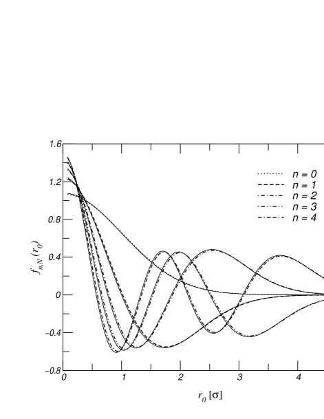
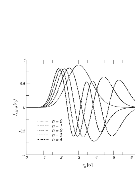
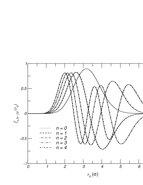
FIG. 1.: The normalized weighting functions for angular momenta $l=N,N-1,N-9,N-10$. These are the eigenfunctions of matrices with $250\times 250$ elements at the system size $R=10$. The normalization condition is $\int drf_{n,l}(r)^{2}=1$. The solid lines are the corresponding radial wave functions of an electron. The only adjustable parameter for the solid curves is the normalization constant.

FIG. 2.: The energy spectrum corresponding to the cyclotron motion of a vortex relative to the lowest energy level. The dotted lines show the scaling of each energy level with the system radius $R$ ranging from $20\sigma$ to $10^{6}\sigma$. The lowest energy level approximately scales as $\ln(R/\sigma)$ corresponding to the formation energy of a vortex. The same spectrum is obtained for any given angular momentum.

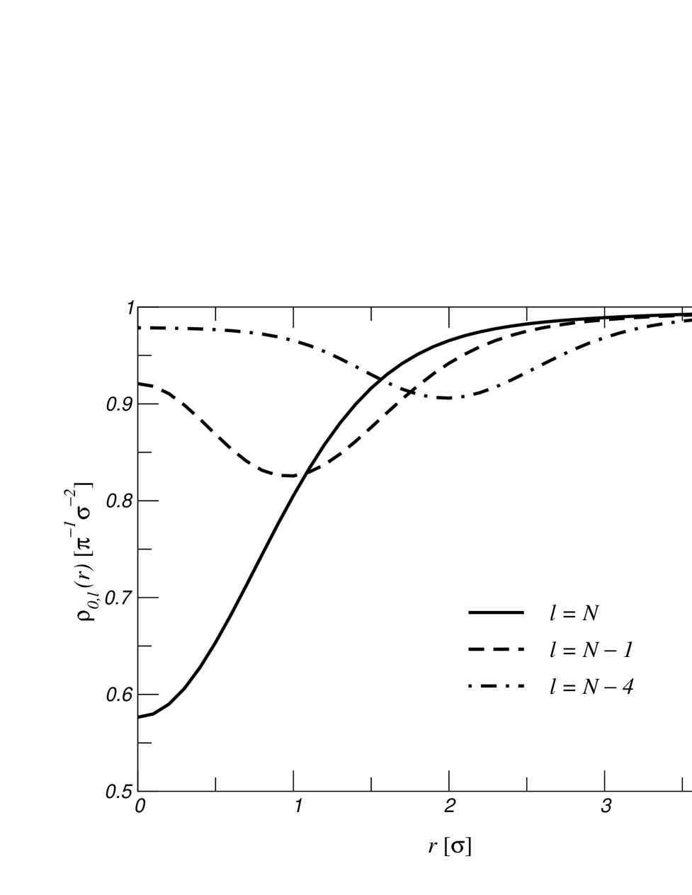
FIG. 3.: The radial profiles of the number density for three different states, each of which has total angular momentum $N$, $N-1$, and $N-4$, in the first Landau level. The curves represent the numerical results in a finite system with radius $R=10$. The limit for all states in the infinite system is uniform density. Instead of fixing the total number of particles, the normalization is chosen in such a way that the asymptotic value is unity.

FIG. 4.: The radial profiles of the azimuthal current density for three different states, each of which has total angular momentum $N$, $N-1$, and $N-4$, in the first Landau level. The dashed lines represent the numerical results in a finite system with radius $R=10$, and the solid lines represent the results for the infinite-system limit. The dotted line is the classical result for a singular vortex line.

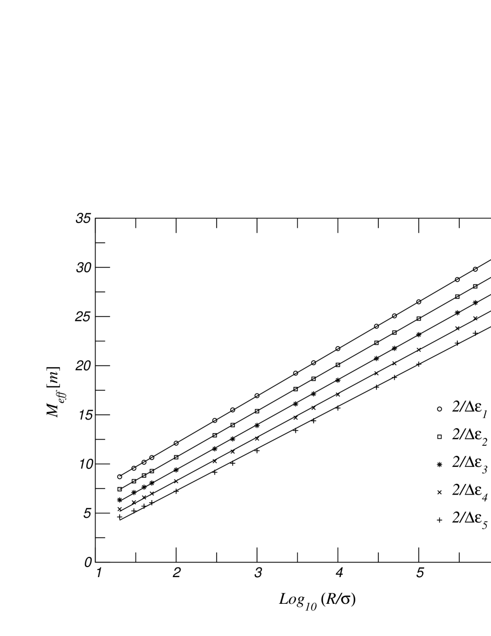
FIG. 5.: The scalings of the inverse of energy-level spacings labeled as $\Delta\varepsilon_{n}=\varepsilon_{n}-\varepsilon_{n-1}$, which are related to the effective mass of a vortex. The symbols show the first five of them from top to bottom. The lines are the least-square fits, and clearly show that the effective mass scales logarithmically with the vortex size $R$.

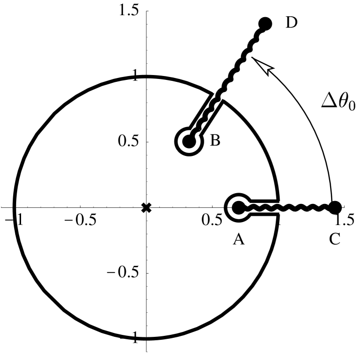
FIG. 6.: Branch points, $A$ to $D$, branch cuts, $\overline{AC}$ and $\overline{BD}$, and the integration contour deformed from the unit circle. This particular sequence of the branch points corresponds to the case $r>r_{0},r^{\prime}_{0}$. There may be a simple pole located at the origin depending on which integrand is discussed.

REFERENCES

- [1] L. Onsager, Suppl. Nuovo Cimento 6, 249 (1949).
- [2] R. P. Feynman, in Progress in Low Temperature Physics, edited by C. J. Gorter (Elsevier Science Publishers B.V., Amsterdam, 1955), Vol. 1, Chap. 2, pp. 17–53.
- [3] M. Hatsuda, S. Yahikozawa, P. Ao, and D. J. Thouless, Phys. Rev. B 49, 15870 (1994).
- [4] S. H. Lamb, Hydrodynamics (The University Press, Cambridge, 1932).
- [5] R. J. Donnelly, Quantized Vortices in Helium II (Cambridge University Press, New York, 1991).
- [6] von Klitzing, K. G. Dorda, and M. Pepper, Phys. Rev. Lett. 45, 494 (1980).
- [7] R. A. Ashton and W. L. Glaberson, Phys. Rev. Lett. 42, 1062 (1979).
- [8] H. D. Drew and T. C. Hsu, Phys. Rev. B 52, 9178 (1995).
- [9] T. Ichiguci, Phys. Rev. B 57, 638 (1998).
- [10] D. L. Hill and J. A. Wheeler, Phys. Rev. 89, 1102 (1953).
- [11] R. E. Peierls and J. Yoccoz, Proc. Roy. Soc. A 70, 381 (1957).
- [12] R. E. Peierls and D. J. Thouless, Nucl. Phys. 38, 154 (1962).
- [13] G. Ortiz and D. M. Ceperley, Phys. Rev. Lett. 75, 4642 (1995).
- [14] S. Giorgini, J. Boronat, and J. Casulleras, Phys. Rev. Lett. 77, 2754 (1996).
- [15] S. A. Vitiello, L. Reatto, G. V. Chester, and M. H. Kalos, Phys. Rev. B 54, 1205 (1996).
- [16] M. Sadd, G. V. Chester, and L. Reatto, Phys. Rev. Lett. 79, 2490 (1997).
- [17] R. P. Feynman, Phys. Rev. 91, 1301 (1953).
- [18] G. V. Chester, R. Metz, and L. Reatto, Phys. Rev. 175, 275 (1968).
- [19] R. P. Feynman and M. Cohen, Phys. Rev. 102, 1189 (1956).
- [20] P. G. Saffman, Vortex Dynamics (Cambridge University Press, New York, 1995).
- [21] R. P. Feynman, Phys. Rev. 94, 262 (1954).
- [22] B. E. Clements, J. L. Epstein, E. Krotscheck, and M. Saarela, Phys. Rev. B 48, 7450 (1993).
- [23] A. L. Fetter, Phys. Rev. Lett. 27, 986 (1971).
- [24] J. M. Duan, Phys. Rev. B 49, 12381 (1994).
- [25] J. M. Duan, Phys. Rev. Lett. 75, 974 (1995).
- [26] Q. Niu, P. Ao, and D. J. Thouless, Phys. Rev. Lett. 72, 1706 (1994).
- [27] Q. Niu, P. Ao, and D. J. Thouless, Phys. Rev. Lett. 75, 975 (1995).
- [28] L. D. Landau and E. M. Lifshitz, Quantum Mechanics: Non-Relativistic Theory, 3rd ed. (Pergamon, Oxford, 1977).