Parafermion Statistics and Quasihole Excitations for the Generalizations of the Paired Quantum Hall States

Abstract

We continue the program started in [7] and explain the statistics of the excitations for the generalizations of the paired states in the quantum Hall effect in terms of the parafermion statistics. We show that these excitations behave as combinations of bosons and parafermions. That generalizes the prior treatment of the paired (Pfaffian) state where the excitations behave as combinations of bosons and fermions. We explain what it means, from a quantum mechanical point of view, for a particle to be a ‘parafermion’ rather than a boson or a fermion and work through several explicit examples. The resulting multiplets coincide exactly with the angular momentum multiplets found numerically for the $k+1$ particle interaction Hamiltonian on a sphere. We also present a proof that the wave functions found in [7] are indeed the correlation functions of the parafermion conformal field theory.

I Introduction

The quantum Hall plateaus on the first excited Landau levels appear to be different from those of the lowest Landau level. The most striking difference is the $5/2$ plateau [1] for which there is no analog in the lowest Landau level.

To explain the $5/2$ plateau, several trial wave functions were proposed. One of them, the Haldane-Rezayi state [2], assumes that the electrons in it are spin unpolarized. Yet another trial wave function, the Pfaffian [3], assumes that electrons are polarized, just as for the ordinary Laughlin trial wave functions [4]. Recent numerical evidence [5, 6], in the absence of the Landau level mixing, supports the Pfaffian as a trial wave function for the $5/2$ plateau.

In the paper by N. Read and one of us [7] a further generalization of the Pfaffian state was proposed. Moreover, it was conjectured, and supported by the numerical evidence, that these generalizations may be better candidates for other plateaus on the first excited Landau levels than the Laughlin state and its hierarchical [4, 8, 9] or composite fermion [10] generalizations.

An unusual feature of the generalizations of the Pfaffian state given in [7] was that the trial wave functions were found explicitly for nonsimple fractions. That was done with the help of conformal field theory.

Conformal field theory discovered in [11] is essentially a method to solve various scale invariant 1+1 dimensional quantum field theories exactly. It was since proved extremely useful for understanding various 1 dimensional quantum and 2 dimensional classical statistical mechanics systems. Its relevance for the quantum Hall systems was first discussed in [3].

The relevant conformal field theory for the generalization of the Pfaffian is the so-called parafermion conformal field theory [12]. The parafermions, the direct generalizations of the fermions, play an important role in describing the critical points of the $Z_{k}$ invariant statistical mechanics systems. A particularly well known example of the $Z_{2}$ invariant system is the Ising model. The Ising model can be described by a Majorana fermion. A $Z_{k}$ invariant system must be described, on the other hand, by $Z_{k}$-parafermions.

A Majorana fermion $\psi(z)$ can be used to generate the Pfaffian trial wave function, as was discussed in [3].

$$\Psi_{\rm Pfaffian}=\langle\psi(z_{1})\psi(z_{2})\dots\psi(z_{N})\rangle\prod_{i<j\leq N}(z_{i}-z_{j})^{2}$$ (1)

The filling factor of this trial wave function is $1/2$. Moreover, the so-called spin fields of the fermion conformal field theory (the order parameter of the Ising model) $\sigma$ can be used to generate the excitations of such a system,

$$\Psi_{\rm Pfaffian}^{\rm excited}(\eta_{1},\eta_{2},\dots,\eta_{2L})=\langle\sigma(\eta_{1}),\sigma(\eta_{2}),\dots,\sigma(\eta_{2L}),\psi(z_{1}),\psi(z_{2}),\dots,\psi(z_{N})\rangle\prod_{i,j}(\eta_{i}-z_{j})^{1\over 2}\prod_{i<j}(z_{i}-z_{j})^{2}.$$ (2)

On the other hand, as was discussed in [12], for each $k$ there are $k-1$ parafermions, denoted $\psi_{l}$, with dimensions $h_{k}=l(k-l)/k$. In [7] it was proposed to use the first of them to generate a parafermion wave function,

$$\Psi_{\rm para}^{M}=\langle\psi_{1}(z_{1})\psi_{1}(z_{2})\dots\psi_{1}(z_{N})\rangle\prod_{i<j\leq N}(z_{i}-z_{j})^{M+{2\over k}}$$ (3)

where $M$ has to be taken odd or even integer depending on whether the particles are fermions or bosons. The filling factor of this wave function is given by $\nu=k/(kM+2)$.

It was further shown in [7] that this wave function should be an exact ground state of a system of $N$ bosons in a magnetic field in the presence of the $k$-body interaction Hamiltonian

$$H=V\sum_{i_{1}<i_{2}<\dots<i_{k+1}}\delta^{2}(z_{i_{1}}-z_{i_{2}})\delta^{2}(z_{i_{2}}-z_{i_{3}})\dots\delta^{2}(z_{i_{k}}-z_{i_{k+1}}),$$ (4)

thereby generalizing the Pfaffian case for which the interaction Hamiltonian was (4) at $k=2$. We do not need to consider fermions because their wave function can be obtained from that of bosons by a simple Jastrow factor.

To find the wave function directly from (3) is a difficult task. However, it was shown in [7] that the following explicit construction has the correct properties (it is symmetric and vanishes whenever $k+1$ particles coincide), which we reproduce for future reference.

To write down $\Psi_{\rm para}^{(0)}$ we need to break the coordinates of $N$ electrons into clusters of $k$ ($N$ should be divisible by $k$). For each pair of distinct clusters, say $z_{1},\dots,z_{k}$ and $z_{k+1},\dots,z_{2k}$, we define factors $\chi$ by

$$\chi_{1,2}(z_{1},\dots,z_{k};z_{k+1},\dots,z_{2k})=(z_{1}-z_{k+1})(z_{1}-z_{k+2})(z_{2}-z_{k+2})(z_{2}-z_{k+3})\dots(z_{k}-z_{2k})(z_{2k}-z_{k+1}).$$ (5)

The subscript $1,2$ of $\chi_{1,2}$ labels the clusters (the first, starting with $z_{1}$ and the second, starting with $z_{k}$).

The wave function $\Psi_{\rm para}^{(0)}$ is defined in terms of these as

$$\Psi_{\rm para}^{(0)}=\sum_{P}\prod_{0\leq r<s<N/k}\chi_{r+1,s+1}(z_{P(kr+1)},\dots,z_{P(k(r+1))};z_{P(ks+1)},\dots,z_{P(k(s+1))}).$$ (6)

It is not hard to see that for $k=2$ this wave function reproduces the Pfaffian for bosons at $\nu=1$.

It was also observed in [7] that the quasihole excitations above (6) can be described by the insertion of the spin fields $\sigma_{1}$ of the parafermion conformal field theory. While some of the excitations for the Pfaffian state were found explicitly in [13], no explicit wave functions for the excitations of the parafermion states have yet been found.

The purpose of this paper is to continue the work begun in [7]. In particular, we explain the numerically observed degeneracies of the excitations of the parafermion states. It turns out that to reproduce the numerically observed degeneracies we need to assume that these excitations obey the parafermion statistics.

Here we would like to emphasize that although the parafermions have been shown in [15] to obey the Haldane exclusion principle [16] in the statistical sense which is a valid description for large quantities of parafermions, for small number of parafermions we need to know the concrete rules which govern the combinatorics of parafermions. These rules asymptotically approach the exclusion statistics rules as the number of parafermions becomes large. These rules are described below and by themselves do not have much to do with Haldane exclusion statistics.

Our finding that the excitations of the parafermion states behave as a combination of bosons and parafermions is a direct generalization of the well known fact that the excitations of the Pfaffian state behave as a combination of bosons and fermions.

We also show that the wave function (6) is indeed given by the parafermion correlation function (3), thus confirming the conjecture of [7].

II Excitations of the $Z_{3}$-Parafermion State on a Sphere

In this section we are going to explain how to calculate the degeneracy of the excitations of the parafermion states. To do that, we will have to construct what could be called parafermion quantum mechanics and learn how to add angular momenta of the quantum mechanical particles obeying parafermion statistics.

It was shown in [7] that if you put $N$ particles on a sphere with a magnetic monopole in the center, turn on $k+1$ particle interaction (4) and then adjust the total flux of the magnetic field through the surface of the sphere to be equal to $N_{\phi}=\nu^{-1}N-(M+2)$ with $\nu$ being the filling factor, $\nu=k/(Mk+2)$ and $M$ being either odd (for fermions) or even (for bosons) nonnegative integer, you discover that the electrons settle into one unique zero energy ground state with the wave function

$$\Psi_{\rm GS}=\prod_{i<j}(z_{i}-z_{j})^{M}\Psi(z_{1},\dots,z_{N}),$$ (7)

with $\Psi(z_{1},\dots,z_{N})$ given by (6). The total angular momentum of that state is equal to $0$.

Now if you start increasing the flux by units of one flux quanta, you discover that the zero energy eigenstates of (4) are degenerate. These states can all be grouped into the angular momentum multiplets.

The reason for this is more or less clear. By increasing the flux by 1, we create quasiholes. There is more than one way of creating those quasiholes which explains the degeneracy of states at a higher flux.

As was explained in [7] the elementary quasiholes at arbitrary $k$ are not Laughlin quasiholes. Rather, they are quasiholes which carry flux $1/k$ and we create $k$ of them at once. The wave functions with quasiholes can be found with the help of conformal field theory, by inserting the fields $\sigma_{1}$ of the parafermion conformal field theory [12, 7]. However, we are not going to be interested in the explicit wave functions.

What we want to explain in this section is the numerically observed degeneracy of the states with quasiholes on a sphere and how exactly one could generate all the degeneracies. We will show how the correct angular momentum multiplets can be obtained by putting parafermions into orbitals on a sphere and combining their angular momenta in a way consistent with their fractional statistics. That generalizes the prior treatment of the Pfaffian state in [14].

Now we would like to present, first without explanation, the rules for finding the degeneracies of the excitations above the $k=3$ state, that is, for $Z_{3}$-parafermions.

It was found in [7], by matching the numerical data, that, as we increase the flux, the degeneracy of states we get for the $Z_{3}$ parafermions is given by the following formulas. The number of excitations at the excess flux 1 (3 quasiholes, each carrying $1/3$ of the flux quantum) is given by a binomial coefficient

$${{N/3+3}\choose 3},$$ (8)

with $N$ being the total number of the electrons. $N$ should be divisible by three. This coefficient has a simple interpretation as the number of ways you can put 3 bosons into $N/3+1$ orbitals. The reason why the excitations at the excess flux $1$ behave as bosons was explained in [7] and is essentially the same for the parafermion states as for the Pfaffian state [14].

Moreover, following [14], we can assign the angular momentum quantum numbers to these states. For this purpose we interpret the $N/3+1$ states as the orbitals on a sphere, in the multiplet of the angular momentum $L=N/6$. When we put the bosons on this sphere, we generate the angular momentum multiplets by combining their angular momenta while keeping their wave function totally symmetric.

While we could refer to any standard quantum mechanics textbooks for the rules on how to combine the angular momenta of bosons, we can recast these rules into the following simple form. Let us visualize $N/3+1$ orbitals as boxes. Each box has a number $L_{z}$ assigned to it which varies from $-N/6$ to $N/6$ by steps of $1$. We are allowed to put as many bosons as we wish into each particular box.

For example, for $N=6$ we have $3$ boxes with $L_{z}=-1$, $L_{z}=0$, and $L_{z}=1$. Fig. 1 shows one possible way to put 3 bosons into 3 boxes, by putting 2 of them into $L_{z}=1$ box and one into $L_{z}=-1$ box, thus giving the total $L_{z}=1$. Of course, there are ${5\choose 3}=10$ ways to put 3 bosons into 5 boxes. Out of these 10 ways, the angular momentum projections $L_{z}=\pm 3$ or $L_{z}=\pm 2$ can be obtained in 1 way each, while the angular momentum projections $L_{z}=\pm 1$ or $L_{z}=0$ can be obtained in 2 different ways each. We immediately recognize the sum of the $L=3$ and $L=1$ angular momentum multiplets. And indeed, this is confirmed by the numerical data.

FIG. 1.: One possible way to put 3 bosons into 3 boxes, realizing (8) for $N=6$

As the flux is increased we observe many more excited states. It was found in [7] that the number of states at the excess flux $2$ is given by

$${{N/3+6}\choose 6}+3{{N/3+5}\choose 6}+{{N/3+4}\choose 6},$$ (9)

and at the three excess flux quanta

$${{N/3+9}\choose 9}+10{{N/3+8}\choose 9}+10{{N/3+7}\choose 9}.$$ (10)

The higher fluxes turned out to be harder to analyze as there is less numerical data available for them.

We observe that the number of states at these flux quanta is reminiscent of the corresponding formula for the Pfaffian which was found in [14] to be

$$\sum_{F,(-1)^{F}=(-1)^{N},F\leq N}{n\choose F}{{(N-F)/2+2n}\choose{2n}}$$ (11)

with $n$ being the number of the excess flux quanta. The extra $n\choose F$ was interpreted as the number of ways one can put $F$ fermions into $n$ boxes. By analogy, we can write down a formula which generalizes (11) to the case of the $k=3$ parafermions,

$$\sum_{F\geq 0,\exp\left(2\pi Fi\over 3\right)=1,F\leq N}\left\{{n\above 0.0ptF}\right\}{{(N-F)/3+3n}\choose{3n}}$$ (12)

where $\left\{{n\above 0.0ptF}\right\}$ is the number of ways you can put $F$ $Z_{3}$-parafermions into $n$ orbitals.

What does it exactly mean, to put parafermions into orbitals? Inspired by the parafermion mode counting derived in [15], we present the following rules. While the rules are relatively complicated, they are the only way known to us which allows to obtain $\left\{{n\above 0.0ptF}\right\}$ and, at the same time, to break the configurations into angular momentum multiplets.

We replace the boxes by the ‘positions’. As we move from right to left, each next position carries $1/3$ more of the $z$-component of the angular momentum, as in Fig. 2, ranging from $-(3n-2)/6$ to $(3n-2)/6$. Thus, we have $3n-1$ positions. Fig. 2 depicts the positions at $n=2$.

FIG. 2.: Positions where the parafermions are to be put for $n=2$

There are two types of the $Z_{3}$-parafermions we can put into these positions. We depict them by either the light shaded or dark shaded circles. The following rules should be used to put the parafermions into the positions:

1. The light shaded circle carries $L_{z}$ equal to the $L_{z}$ of its position.

2. The dark shaded circle carries $L_{z}$ equal to twice the $L_{z}$ of its position. In addition, the dark shaded circle is counted as two parafermions.

3. The dark shaded parafermion can occupy any position, while the light shaded parafermion is not allowed to occupy the rightmost or the leftmost position. The number of empty positions to the left of the leftmost parafermion has to be $3l$ if it is dark shaded, or $3l+1$ if it is light shaded, where $l$ is any nonnegative integer, including $0$. For example, if the leftmost parafermion is the light shaded one, it can occupy the position number $2$, or $5$, or in general $2+3l$ counting from the left, and if it is a dark shaded one, it can occupy the position number $1$, or $4$, $\dots$.

4. The adjacent light shaded parafermions are allowed to have $3l$ empty positions between them, while the adjacent dark shaded parafermions have to have $3l+1$ empty positions between them. If a light shaded parafermions is adjacent to a dark shaded parafermion, they have to be separated by $3l+2$ empty positions, where $l$ is any nonnegative integer including $0$.

Examples of the allowed configurations are shown on Fig. 3. This figure depicts the $3$ ways one can put $3$ parafermions into $5$ positions at $n=2$, consistent with (9) and (12). Moreover, we immediately observe that these configurations form an $L=1$ multiplet.

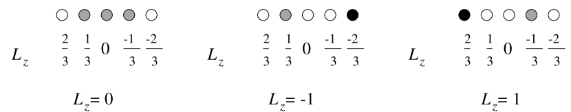
FIG. 3.: Three possible ways one can put 3 $Z_{3}$-parafermions into 2 boxes, in accordance with $\left\{{2\above 0.0pt3}\right\}=3$.

It is not very convenient to draw positions all the time, so we introduce the following compact notations. Each light circle will be represented by $\psi_{s}$ with $s$ equal to $L_{z}$ of the circle. Each dark circle will be represented by $\phi_{s}$. For example, the three configurations of the Fig. 3 can be represented as

$$\psi_{1\over 3}\psi_{0}\psi_{{-1\over 3}},\ \ \psi_{1\over 3}\phi_{{-2\over 3}},\ \ \phi_{2\over 3}\psi_{{-1\over 3}}$$ (13)

(we remember that in accordance with the rule 2, $\phi$ is counted as two parafermions).

There is only one way to put $6$ parafermions into $5$ positions at $n=2$,

$$\phi_{2\over 3}\phi_{0}\phi_{{-2\over 3}},$$ (14)

consistent with $\left\{{2\above 0.0pt6}\right\}=1$.

Let us demonstrate the power of the technique by breaking the $n=3$ configurations into multiplets. There should be $8$ positions, carrying $L_{z}$ from $-7/6$ to $7/6$, that is, $-7/6$, $-5/6$, $-3/6$, $-1/6$, $1/6$, $3/6$, $5/6$, and $7/6$.

It is obvious there is only $1$ way to put zero parafermions into these positions.

According to (10) and (12) $\left\{{3\above 0.0pt3}\right\}=10$. Indeed, we can count the configurations directly

$$L_{z}\left(\psi_{5\over 6}\psi_{3\over 6}\psi_{1\over 6}\right)={3\over 2},\ \ L_{z}\left(\psi_{5\over 6}\psi_{3\over 6}\psi_{-5\over 6}\right)={1\over 2},\ \ L_{z}\left(\psi_{5\over 6}\psi_{-3\over 6}\psi_{-5\over 6}\right)=-{1\over 2},\ \ L_{z}\left(\psi_{-1\over 6}\psi_{-3\over 6}\psi_{-5\over 6}\right)=-{3\over 2},$$ (15)

$$L_{z}\left(\phi_{7\over 6}\psi_{1\over 6}\right)={5\over 2},\ \ L_{z}\left(\phi_{7\over 6}\psi_{-5\over 6}\right)={3\over 2},\ \ L_{z}\left(\phi_{1\over 6}\psi_{-5\over 6}\right)=-{1\over 2},$$ (16)

$$L_{z}\left(\psi_{5\over 6}\phi_{-1\over 6}\right)={1\over 2},\ \ L_{z}\left(\psi_{5\over 6}\phi_{-7\over 6}\right)=-{3\over 2},\ \ L_{z}\left(\psi_{-1\over 6}\phi_{-7\over 6}\right)=-{5\over 2}.$$ (17)

We observe $10$ different configurations. Moreover, we observe that $L_{z}=\pm 5/2$ occurs only once each, and $L_{z}=\pm 3/2$ or $L_{z}=\pm 1/2$ occurs twice each. We immediately recognize the sum of $L=5/2$ and $L=3/2$ angular momentum multiplets.

Quite analogously, for $6$ parafermions at $n=3$ we find

$$L_{z}\left(\psi_{5\over 6}\psi_{3\over 6}\psi_{1\over 6}\psi_{-1\over 6}\psi_{-3\over 6}\psi_{-5\over 6}\right)=0,$$ (18)

$$L_{z}\left(\psi_{5\over 6}\psi_{3\over 6}\psi_{1\over 6}\psi_{-1\over 6}\phi_{-7\over 6}\right)={-1},\ \ L_{z}\left(\phi_{7\over 6}\psi_{1\over 6}\psi_{-1\over 6}\psi_{-3\over 6}\psi_{-5\over 6}\right)=1,$$ (19)

$$L_{z}\left(\phi_{7\over 6}\phi_{3\over 6}\psi_{-3\over 6}\psi_{-5\over 6}\right)=2,\ \ L_{z}\left(\psi_{5\over 6}\psi_{3\over 6}\phi_{-3\over 6}\phi_{-7\over 6}\right)=-2,\ \ L_{z}\left(\phi_{7\over 6}\psi_{1\over 6}\psi_{-1\over 6}\phi_{-7\over 6}\right)=0,$$ (20)

$$L_{z}\left(\phi_{7\over 6}\phi_{3\over 6}\phi_{-1\over 6}\right)=3,\ \ L_{z}\left(\phi_{7\over 6}\phi_{3\over 6}\phi_{-7\over 6}\right)=1,\ \ L_{z}\left(\phi_{7\over 6}\phi_{-3\over 6}\phi_{-7\over 6}\right)=-1,\ \ L_{z}\left(\phi_{1\over 6}\phi_{-3\over 6}\phi_{-7\over 6}\right)=-3.$$ (21)

The total multiplicity is $10$, in agreement with (10). Counting $L_{z}$ we observe that $L_{z}=\pm 3$ and $L_{z}=\pm 2$ occurs in one configuration each, while $L_{z}=\pm 1$ and $L_{z}=0$ occurs twice each. We recognize the direct sum of $L=3$ and $L=1$ multiplets.

One can further check that it is impossible to fit $9$ or more parafermions into these positions.

The Tables I, II, and III in the appendix below contain the numerical data available for the Hamiltonian (4) at $k=3$ and at the number of electrons fixed at $N=6$, $N=9$ and $N=12$. The data is in the form $L$ versus $n$. For each excess flux quanta $n$ the intersection of $n$th column and $L$th row contains the multiplicity of the angular momentum $L$ at given $n$.

To reproduce this data using the parafermion counting rules, we need to combine the angular momenta of the parafermions with those of bosons, by analogy with (12). This is now trivial to do, since parafermions and bosons are distinguishable particles, and their angular momenta combine in accordance with standard rules.

For example, at $N=6$ we can obtain the multiplets in the following way. First we need to put $9$ bosons into $3$ orbitals as represented by the term of (12) with $F=0$. Their angular momenta are calculated in exactly the same way as we calculated the angular momenta for $3$ bosons in $3$ orbitals in the text directly preceding Fig. 1.

Then we have to put $9$ bosons into $2$ orbitals and combine their angular momenta with the $L=5/2$ and $L=3/2$ angular momenta of the parafermions, as represented by the term of (12) with $F=3$.

And finally, we put $9$ bosons into $1$ orbital. There is only one such state and its angular momentum is $0$. Therefore the total angular momentum is just $L=3$ and $L=1$, coming from the parafermion contribution.

We are not going to go through explicit counting since it is rather standard. The only nontrivial step was the parafermion angular momentum contribution, and that was worked out above. We have checked, however, that the result reproduces the numerical data given in the Table I. In fact, we have verified all the data in all three Tables, expect the results for $n=5$ at $N=6$. In particular, we found that the parafermion multiplets at $n=4$ are the following. At $F=3$, there is one each of $L=0,2,3,4$ states giving the multiplicity of $22$ (compare with (25)). At $F=6$, there are two each of $L=0,2,4$ states, and one each of $L=3,6$ states giving the overall multiplicity of $50$. For $F=9$ it is one of each $L=0,2,4$, with a total multiplicity of $15$. And for $F=12$ there is one $L=0$ state.

It would be nice if we could obtain the parafermion multiplicities $\left\{{n\above 0.0ptF}\right\}$ in a more closed form rather than by having to count configurations all the time. The most closed form that we are aware of can be obtained with the help of the equation for the partial partition functions derived in [15].

We define the polynomials $Y_{l}(x)$ in the following way.

$$Y_{l+1}(x)=xY_{l+{2\over 3}}(x)+x^{2}Y_{l+{1\over 3}}(x)+(1-x^{3})Y_{l}(x),$$ (22)

with the initial conditions $Y_{-{1\over 3}}=0$, $Y_{0}=1$, and $Y_{1\over 3}=0$. Then we claim that the following expansion is valid

$$Y_{n}(x)=\sum_{k=0,1,\dots}\left\{{n\above 0.0pt3k}\right\}x^{3k}.$$ (23)

It is in fact possible to derive (22) directly from the counting rules presented above, see [15].

It is not hard to check that

$$Y_{1}=1,\ \ Y_{2}=1+3x^{3}+x^{6},\ \ Y_{3}=1+10x^{3}+10x^{6}$$ (24)

in agreement with (9) and (10). We can continue further,

$$Y_{4}=1+22x^{3}+50x^{6}+15x^{9}+x^{12},\ \ Y_{5}=1+40x^{3}+168x^{6}+140x^{9}+28x^{12}.$$ (25)

These multiplicities are also in agreement with the available numerical data for the degeneracies at various flux quanta $n$.

We note that according to [7] the sum of the multiplicities at fixed $n$ should give us Fibonacci numbers $F_{3n-2}$,

$$\sum_{k=0,1,2,\dots}\left\{{n\above 0.0pt3k}\right\}=F_{3n-2}.$$ (26)

That is indeed true, since this sum is equal to $Y_{n}(1)$, and by substituting $x=1$ into (22) we obtain

$$Y_{l+1}(1)=Y_{l+{2\over 3}}(1)+Y_{l+{1\over 3}}(1),$$ (27)

which is the defining relation for the Fibonacci numbers.

III Conformal Field Theory and the Counting Rules

The rules we have just presented were in fact deduced from the parafermion conformal field theory. Here we would like to explain how conformal field theory should be employed to derive these rules.

While we were interested in parafermion quantum mechanics, conformal field theory, as a field theory, gives us the counting rules in the second quantized formalism. It is not so hard to read statistics off the second quantized formalism.

Let us concentrate on the Majorana fermions as an example. We know, of course, that there are $n\choose F$ ways to put $F$ fermions into $n$ boxes, in accordance with Pauli exclusion principle. This can be obtained also from the conformal field theory of the Majorana fermions.

Expanding the Majorana fermion $\psi_{n}$ in terms of modes we get

$$\psi(z)=\sum_{n}\psi_{n}z^{-n-{1\over 2}},$$ (28)

with $n$ going over half integers $1/2+Z\!\!\!Z$. The modes $\psi_{n}$ obey the anticommutation relations,

$$\psi_{n}\psi_{m}+\psi_{m}\psi_{n}=\delta_{n+m,0}.$$ (29)

All these are well known facts of conformal field theory.

Since the Majorana fermion defined at every point in space and time cannot be infinite when acting on the vacuum, $\psi(z)|0\rangle$ for any $z$ including $z=0$, it follows that $\psi_{n}|0\rangle=0$ for all $n=1/2,3/2,\dots$. We say that the modes of $\psi(z)$ with positive index act as annihilation operators. The modes $\psi_{n}$ with $n=-1/2,-3/2,\dots$ act as creation operators. We can use them to create new states. A generic state will look like

$$\psi_{-n_{F}}\psi_{-n_{F-1}}\dots\psi_{-n_{1}}|0\rangle,$$ (30)

with all the $n_{i}$ being negative half integers. Note that some of the states in (30) are not linearly independent and can actually be transformed into each other by repeatedly using the anticommutation relations (29). We can select a linear independent subset of (30) by ordering all the $n$, say making them increase from left to right, and making sure neither of them are equal to each other, thereby making the state zero according to $\psi_{n}^{2}=0$.

Now observe that there is the following correspondence between the states (30) and the angular momentum wave functions. Consider the states (30) together with the relevant powers of the coordinates, as in (28).

$$\psi_{-n_{F}}\psi_{-n_{F-1}}\dots\psi_{-n_{1}}|0\rangle\ z_{1}^{n_{F}-{1\over 2}}z_{2}^{n_{F-1}-{1\over 2}}\dots z_{F}^{n_{1}-{1\over 2}}.$$ (31)

Let us now sum (31) over all the states accessible via the anticommutation relations (29). In other words, we want to sum over all the permutations $\sigma$ of the numbers $n_{1}$, $n_{2}$, $\dots$, $n_{F}$. Obviously we obtain

$$\sum_{\sigma}\psi_{-\sigma(n_{F})}\psi_{-\sigma(n_{F-1})}\dots\psi_{-\sigma(n_{1})}|0\rangle\ z_{1}^{\sigma(n_{F})-{1\over 2}}z_{2}^{\sigma(n_{F-1})-{1\over 2}}\dots z_{F}^{\sigma(n_{1})-{1\over 2}}=$$ (32)

$$\psi_{-n_{F}}\psi_{-n_{F-1}}\dots\psi_{-n_{1}}|0\rangle\ \sum_{\sigma}{\rm sign}(\sigma)\ z_{1}^{\sigma(n_{F})-{1\over 2}}z_{2}^{\sigma(n_{F-1})-{1\over 2}}\dots z_{F}^{\sigma(n_{1})-{1\over 2}}.$$ (33)

One immediately recognizes the totally antisymmetric polynomials of the sort discussed in [14]. The angular momentum $L_{z}$ computed on these polynomials can be defined, up to an additive constant, as generated by the operator $z{\partial\over\partial z}$, to give $\sum_{i}n_{i}-F/2$. These totally antisymmetric polynomials are in fact the wave functions of the fermions in the first quantized formalism!

If we consider all possible states (32), with the restrictions $n_{N}<n$, $n$ being some integer, there is going to be exactly $N\choose F$ of them which are the multiplicities in (11). Now we see how these states break naturally into angular momentum multiplets. One can check that the multiplets we obtain in this way matches the numerical data for the Pfaffian state [14].

What we just did so far looks like a complicated and not very intuitive way of rederiving the results of [14]. However, as we move on to the parafermion states, conformal field theory becomes the only consistent and dependable way to construct the angular momenta multiplets.

$k=3$ parafermion conformal field theory contains two fields of dimension $2/3$, $\psi^{(1)}(z)$ and $\psi^{(2)}(z)$ [12]. Expanding them in terms of modes we obtain

$$\psi^{(1)}(z)=\sum_{n}\psi^{(1)}_{n}z^{-n-{2\over 3}},\ \ \psi^{(2)}(z)=\sum_{n}\psi^{(2)}_{n}z^{-n-{2\over 3}}.$$ (34)

It is obvious that the modes $\psi^{(1)}_{n}$ and $\psi^{(2)}_{n}$ have to annihilate the vacuum if $n>-2/3$. Applying the modes with $n\leq-2/3$ to the vacuum we can in fact create parafermionic states. Not all the states we create in this way are linearly independent. To check which ones are independent we have to employ the generalized commutation relations of the sort derived in [12]. These relations are very complicated. Fortunately for $k=3$ the set of independent states have already been derived in [15]. Here for completeness we are going to quote the answer.

The full set of linearly independent states is created by applying the modes of the parafermions of the first kind $\phi^{(1)}_{s}\equiv\psi^{(1)}_{s}$ or a certain combination of the modes $\phi^{(2)}_{s}\equiv\psi^{(1)}_{s}\psi^{(1)}_{s-{2\over 3}}$. We do not need to use the modes of the parafermion of the second kind $\psi^{(2)}$ as its modes create states which are linearly dependent on the states created by $\phi^{(1)}_{s}$ and $\phi^{(2)}_{s}$.

The allowed states have the form

$$\phi^{\left(i_{N}\right)}_{-s_{N}}\dots\phi^{\left(i_{2}\right)}_{-s_{2}}\phi^{\left(i_{1}\right)}_{-s_{1}}|0\rangle,$$ (35)

with the spacing specified as

$${\rm if}\ \ i_{l+1}=1,\ i_{l}=1\ \ {\rm then}\ \ s_{l+1}-s_{l}=m+{1\over 3},$$ (36)

$${\rm if}\ \ i_{l+1}=2,\ i_{l}=1\ \ {\rm then}\ \ s_{l+1}-s_{l}=m+{2\over 3},$$ (37)

$${\rm if}\ \ i_{l+1}=1,\ i_{l}=2\ \ {\rm then}\ \ s_{l+1}-s_{l}=m+{4\over 3},$$ (38)

$${\rm if}\ \ i_{l+1}=2,\ i_{l}=2\ \ {\rm then}\ \ s_{l+1}-s_{l}=m+{2\over 3},$$ (39)

where $m$ is any nonnegative integer number including $0$.

We note that these states are in one to one correspondence with the counting rules of the previous section. In fact, this is how the counting rules should be derived.

We can go slightly further and conjecture a way to derive the parafermion wave function. We need to consider the sum over all the states which can be obtained from one of the states (35) by the generalized commutation relations

$$\sum_{\rm dependent\ states}\psi^{\left(j_{N}\right)}_{s_{N}}\dots\psi^{\left(j_{1}\right)}_{s_{1}}|0\rangle\ z_{N}^{-s_{N}-{2\over 3}}\dots z_{1}^{-s_{1}-{2\over 3}},$$ (40)

with different $j$ being either $1$ or $2$. By using those generalized commutation relations we can in principle bring the sum to the form (compare with (32))

$$\phi^{\left(i_{N}\right)}_{-s_{N}}\dots\phi^{\left(i_{2}\right)}_{-s_{2}}\phi^{\left(i_{1}\right)}_{-s_{1}}|0\rangle\ f(z_{1},\dots,z_{N}).$$ (41)

We interpret $f(z_{1},\dots,z_{N})$ to be the wave function of the parafermions!

While finding $f$ explicitly is beyond the scope of this paper, we note that it indeed combines the single particle states of the form $z^{s}$ into the multiparticle wave function obeying the right particle exchange properties.

One should also in principle be able to derive $f$ from the quasihole wave functions in direct analogy with the corresponding derivation for the Pfaffian state [13, 14]. This also lies beyond the scope of this paper.

At the end we would like to note that for $k>3$ the mode counting rules can also be derived by using the generalized commutation relations of [12]. Some partial results at $k=4$ and $k=5$ are presented in [15].

IV The Correlation Functions of the Parafermion CFTs

All the preceding discussion of this paper was based on the assumption that the wave function (6) can be generated as a correlation function of the parafermions, in the sense of [3].

While it was conjectured in [7] that (6) is such a correlation function, no proof was found. It is important to prove this relationship, otherwise, our manipulations with parafermions lose their relevance.

In this section we would like to present a proof that the wave function found in [7], which is the zero energy state of the $k+1$ particle interaction Hamiltonian (4), is indeed the correlation function of a parafermion conformal field theory. For this purpose we recall that a parafermion conformal field theory [12] consists of $k-1$ fields $\psi_{l}$, $l=1,\dots,k-1$ with the operator product expansion

$$\psi_{l}(z)\psi_{l^{\prime}}(z^{\prime})\propto c_{l,l^{\prime}}(z-z^{\prime})^{-2ll^{\prime}/k}(\psi_{l+l^{\prime}}+\beta_{l,l^{\prime}}(z-z^{\prime})\partial\psi_{l+l^{\prime}}+\dots),$$ (42)

where $c$ and $\beta$ are certain numbers – structure constants. The index $l$ of the fields $\psi_{l}$ in (42) has to be understood in the mod $k$ sense, $\psi_{k+l}\equiv\psi_{l}$. Additionally, $\psi_{0}$ is identified with the unit operator. In that case, $\partial\psi_{0}$ vanishes and therefore, when $l+l^{\prime}=0$ mod $k$, the linear term in (42) proportional to $\beta$ vanishes.

According to the conjecture of [7] the correlation function of $N$ fields $\psi_{1}$ is equal to

$$\left\langle\,\psi_{1}(z_{1})\dots\psi_{N}(z_{N})\,\right\rangle={\Psi(z_{1},z_{2},\dots,z_{N})\over\prod_{i<j}(z_{i}-z_{j})^{2\over k}}$$ (43)

with $\Psi$ given by (6).

To show that the right hand side of (43) is indeed consistent with (42), we will glue $k-1$ parafermions $\psi_{1}$ together to obtain the correlation function with $\psi_{k-1}$. Then we will glue $\psi_{k-1}$ and $\psi_{1}$ together and show that the correlation function is consistent with the fact that

$$\psi_{k-1}(z)\psi_{1}(z^{\prime})\propto(z-z^{\prime})^{-2{k-1\over k}}\psi_{0}+\dots$$ (44)

with a vanishing first derivative $\partial\psi_{0}$.

The proportionality sign in (44) and throughout this section means that an unimportant numerical constant has been dropped.

We start with taking the limit $z_{1}\rightarrow z_{2}$. In that limit the right hand side of (43) is proportional to $(z_{1}-z_{2})^{-2/k}$. This is indeed consistent with the operator product expansions

$$\psi_{1}(z)\psi_{1}(z^{\prime})\propto(z-z^{\prime})^{-{2\over k}}\psi_{2}(z^{\prime})+\dots$$ (45)

By multiplying (43) by $(z_{1}-z_{2})^{2/k}$ and taking $z_{1}\rightarrow z_{2}$ we arrive at the following correlation function

$$\left\langle\,\psi_{2}(z_{2})\psi_{1}(z_{3})\dots\psi_{1}(z_{N})\,\right\rangle\propto{\Psi(z_{2},z_{2},z_{3},\dots,z_{N})\over\prod_{i>2}(z_{2}-z_{i})^{4\over k}\prod_{2<i<j\leq N}(z_{i}-z_{j})^{2\over k}}.$$ (46)

As $z_{2}$ approaches $z_{3}$ the right hand side of (46) has just the right singularity $(z_{2}-z_{3})^{-4/k}$, matching the singularity of (42) as $\psi_{2}$ approaches $\psi_{1}$. Therefore, we continue this process further and take $z_{2}\rightarrow z_{3}$. By doing so we indeed recover the correlation function with the field $\psi_{3}$,

$$\left\langle\,\psi_{3}(z_{3})\psi_{1}(z_{4})\dots\psi_{1}(z_{N})\,\right\rangle\propto{\Psi(z_{3},z_{3},z_{3},z_{4},\dots,z_{N})\over\prod_{i>3}(z_{3}-z_{i})^{6\over k}\prod_{3<i<j\leq N}(z_{i}-z_{j})^{2\over k}}.$$ (47)

It is clear at this point that as we continue ‘gluing’ parafermion fields together at some point we will arrive at

$$\left\langle\,\psi_{k-1}(z_{k-1})\psi_{1}(z_{k})\dots\psi_{1}(z_{N})\,\right\rangle\propto{\Psi(z_{k-1},z_{k-1},\dots,z_{k-1},z_{k},z_{k+1},\dots,z_{N})\over\prod_{i>k-1}(z_{k-1}-z_{i})^{2(k-1)\over k}\prod_{k-1<i<j\leq N}(z_{i}-z_{j})^{2\over k}}.$$ (48)

At this stage we should be careful. By taking $z_{k-1}$ to $z_{k}$ we should be able to recover the identity operator $\psi_{k}\equiv\psi_{0}$. Let us check that this is indeed the case. The main singularity of (48) as $z_{k-1}\rightarrow z_{k}$ is $(z_{k-1}-z_{k})^{-{{k-1}\over k}}$ which indeed matches (42) and therefore,

$$\left\langle\,\psi_{0}(z_{k})\psi_{1}(z_{k+1})\dots\psi_{1}(z_{N})\,\right\rangle\propto{\Psi(z_{k},z_{k},\dots,z_{k},z_{k+1},z_{k+2},\dots,z_{N})\over\prod_{i>k}(z_{k}-z_{i})^{2}\prod_{k<i<j\leq N}(z_{i}-z_{j})^{2\over k}}.$$ (49)

By its definition, the identity operator does not depend on its position, and therefore the right hand side of (49) should not depend on $z_{k}$. To see that, let us recall that in [7] the following theorem was proved. The wave function $\Psi$ for $N$ particles whose first $k$ particles live at the same point $z_{k}$ can be expressed in terms of the wave function for $N-k$ particles in the following way,

$$\Psi(z_{k},z_{k},\dots,z_{k},z_{k+1},\dots,z_{N})\propto\prod_{k<i\leq N}(z_{k}-z_{i})^{2}\Psi(z_{k+1},z_{k+2},\dots,z_{N}).$$ (50)

Substituting (50) to (49) we see that

$$\left\langle\,\psi_{0}(z_{k})\psi_{1}(z_{k+1})\dots\psi_{1}(z_{N})\,\right\rangle\propto{\Psi(z_{k+1},z_{k+2},\dots,z_{N})\over\prod_{k<i<j\leq N}(z_{i}-z_{j})^{2\over k}},$$ (51)

that is, $\psi_{0}$ is indeed an identity operator. The correlation function is insensitive to its insertion. That completes the first part of our proof.

If we continue to expand (48) in powers of $z_{k-1}-z_{k}$ we observe that we should reproduce the operator product expansion (42) with $l+l^{\prime}=0$ mod $k$. In particular, we must see that the linear term of that expansion vanishes, $\beta_{k-1,1}=0$. If this term didn’t vanish, that would mean that in addition to the parafermion fields, the conformal field theory whose correlation function is given by (43) has a dimension 1 operator $J$ which generates a U$(1)$ symmetry (see [12]). Such an operator should be absent in the parafermion theory. Let us check that it is indeed absent.

Continuing the expansion of (48) in powers of $z_{k-1}-z_{k}$ we find that the linear term is obviously proportional to

$${\partial\over\partial z_{k-1}}\left.\left[{\Psi(z_{k-1},z_{k-1},\dots,z_{k-1},z_{k},z_{k+1},\dots,z_{N})\over\prod_{i>k}(z_{k-1}-z_{i})^{2(k-1)\over k}}\right]\right|_{z_{k-1}=z_{k}}.$$ (52)

To show that this term is zero it is sufficient to show that

$$\left.{\partial\over\partial z_{k-1}}\Psi(z_{k-1},z_{k-1},\dots,z_{k-1},z_{k},z_{k+1},\dots,z_{N})\right|_{z_{k-1}=z_{k}}={2(k-1)\over k}\left(\sum_{i>k}{1\over z_{k}-z_{i}}\right)\Psi(z_{k},z_{k},\dots,z_{k},z_{k+1},\dots,z_{N}).$$ (53)

We can further simplify the equality (53) by noting that since $\Psi$ is a symmetric function of its arguments, it is enough to differentiate it with respect to just one variable,

$$\left.{\partial\over\partial z_{k}}\Psi(z_{k-1},z_{k-1},\dots,z_{k-1},z_{k},z_{k+1},\dots,z_{N})\right|_{z_{k-1}=z_{k}}={2\over k}\left(\sum_{i>k}{1\over z_{k}-z_{i}}\right)\Psi(z_{k},z_{k},\dots,z_{k},z_{k+1},\dots,z_{N}).$$ (54)

To prove (54) we again recall the definition of $\Psi(z_{1},\dots,z_{N})$ as given in (6). To construct it, we break all its coordinates into $N/k$ clusters of $k$ coordinates and then sum a certain expression, written in terms of these clusters, over all the permutations of $N$ particles. Let us first look at the right hand side of (54). In accordance with the theorem proved in [7], the only terms which contribute to $\Psi(z_{k},\dots,z_{k},z_{k+1},\dots,z_{N})$ in the sum over permutations (6) are those where all the $z_{k}$ belong to the same cluster. This is how (50) could be derived. Let us now make an assumption, which we will justify later, that the only terms which contribute to the left hand side of (54) when we substitute (6) for $\Psi$ are also those where all the $z_{k-1}$ and $z_{k}$ belong to the same cluster.

It is possible to convince oneself that after some algebra the sum of these terms can be reduced to

$$\Phi=\sum_{r=1}^{k}\sum_{P}\prod_{0<j<N/k}{(z_{k}-z_{P\left(r+kj\right)})(z_{k}-z_{P\left(r+kj+s\left(r\right)\right)})\over(z_{k-1}-z_{P\left(r+kj\right)})(z_{k-1}-z_{P\left(r+kj+s\left(r\right)\right)})}\prod_{k<i\leq N}(z_{k-1}-z_{i})^{2}\prod_{0<j<l<N/k}\chi_{j+1,l+1},$$ (55)

where $P(n)$ gives a permutation of the integer numbers $k+1$, $k+2$, $\dots$, $N$. And $s(n)=n+1$ for $0<n<k$ with $s(k)=1$. $\chi$ are the expressions (5). Note that $\chi$ do not depend on $z_{k-1}$ and $z_{k}$. Applying the derivatives as in (54) we get

$$\left.\frac{\partial}{\partial z_{k}}\Phi\right|_{z_{k-1}=z_{k}}=$$ (56)

$$\sum_{r=1}^{k}\sum_{P}\sum_{0<j<N/k}\left({1\over z_{k}-z_{P\left(r+kj\right)}}+{1\over z_{k}-z_{P\left(r+kj+s\left(r\right)\right)}}\right)\prod_{k<i\leq N}(z_{k}-z_{i})^{2}\prod_{0<j<l<N/k}\chi_{j+1,l+1}=$$ (57)

$${2\over k}\left(\sum_{k<i\leq N}{1\over z_{k}-z_{i}}\right)\left.\Phi\right|_{z_{k-1}=z_{k}}.$$ (58)

The last line in (56) follows from the fact that the summation over $r$ completely symmetrizes the sum in the second line of (56) over all the permutations $P$.

Therefore we have proved (54) on the assumptions that the only terms that contribute are those where the first $k$ coordinates of $\Psi$ belong to the same cluster. To see that it is indeed so, let us recall again that according to the theorem proved in [7] all such term should vanish as $z_{k-1}$ approach $z_{k}$. Since they are polynomials they vanish at least as $z_{k}-z_{k-1}$, or perhaps even faster. If they vanish faster, their derivative with respect to $z_{k}$ with the setting $z_{k-1}=z_{k}$ after differentiation is definitely zero. If, on the other hand, they vanish linearly, then we can argue that for each term vanishing as $z_{k}-z_{k-1}$ there is another permutation of the coordinates different from the first one by exchanging exactly the two coordinates in that difference. This term will be proportional to $z_{k-1}-z_{k}$. After differentiating and setting $z_{k}=z_{k-1}$, these terms will cancel each other.

This concludes the proof that the wave function conjectured in [7] to be the correlation function of the parafermions is indeed the correlation function of the parafermions. This in fact allows us to use the parafermionic conformal field theory to describe the ground states of the hamiltonian (4), as we did throughout this paper.

V Acknowledgements

The authors are grateful to N. Read for important discussions and to K. Schoutens for explaining the results of his paper [15]. This work was initiated and completed during the ITP program “Disorder and Interaction in Quantum Hall and Mesoscopic Systems” and was supported by the NSF grants PHY-94-07194 and DMR-9420560 (ER). ER is also grateful to ITP for an ITP Scholar award.

A Numerical Data

In this appendix we present the numerical data for the degeneracy of the angular momenta multiplets at various excess flux quanta $n$. Columns of the tables are labeled by $n$. Rows are labeled by the angular momentum $L$. The intersection of the $n$th column and $L$th row gives us the degeneracy of the angular momentum $L$ multiplets at a given $n$. The three tables represent the angular momentum multiplets at the total particle number $N=6$, $N=9$, and $n=12$. All the data is at $k=3$.

$L\backslash n$	1	2	3	4	5
0		2		3
1	1		2		4
2		2	1	4	2
3	1	1	4	3	7
4		2	2	6	5
5			3	3	8
6		1	2	6	7
7			2	3	8
8				4	5
9			1	2	7
10				2	4
11					4
12				1	2
13					2
14
15					1

TABLE I.: $N=6.$

$L\backslash n$	1	2	3	4
0				6
1/2	1		2
1		3		5
3/2	1		6
2		1		14
5/2	1		7
3		5		14
7/2			8
4		2		21
9/2	1		9
5		3		17
11/2			9
6		2		23
13/2			7
7		2		18
15/2			8
8				20
17/2			5
9		1		16
19/2			4
10				16
21/2			3
11				10
23/2			2
12				11
25/2			0
13				6
27/2			1
14				5
29/2
15				3
31/2
16				2
33/2
17
35/2
18				1

TABLE II.: $N=9.$

$L\backslash n$	1	2	3
0	1	4	6
1		1	7
2	1	6	16
3	1	4	18
4	1	8	24
5		4	21
6	1	7	27
7		3	22
8		4	22
9		2	18
10		2	17
11			11
12		1	11
13			6
14			5
15			3
16			2
17
18			1

TABLE III.: $N=12.$

REFERENCES

- [1] R.L. Willet, J.P. Eisenstein, H.L. Störmer, D.C. Tsui, A.C. Gossard, and J.H. English, Phys. Rev. Lett. 59 (1997) 1776
- [2] F.D.M. Haldane, E. Rezayi, Phys. Rev. Lett. 60 (1988) 956, 1886
- [3] G. Moore, N. Read, Nucl. Phys. B360 (1991) 362
- [4] R.B. Laughlin, Phys. Rev. Lett. 51 (1983) 605
- [5] R.H.Morf, Phys. Rev. Lett. 80 (1998) 1505
- [6] E. Rezayi, F.D.M. Haldane, “Transitions to the paired Hall states in half-filled Landau levels”, 1998 APS March Meeting abstracts; http://www.aps.org/BAPSMAR98/abs/S3470.html#SQ31.001
- [7] N. Read, E. Rezayi, to be published in Phys. Rev. B; cond-mat/9809384
- [8] F.D.M. Haldane, Phys. Rev. Lett. 72 (1984) 605
- [9] B.I. Halperin, Phys. Rev. Lett. 52 (1984) 1583
- [10] J.K. Jain, Phys. Rev. Lett. 63 (1989) 199
- [11] A. Belavin, A. Polyakov, A. Zamolodchikov, Nucl. Phys. B241 (1984) 333
- [12] A. Zamolodchikov, V.A. Fateev, Sov. Phys. JETP 62 (1985) 215
- [13] C. Nayak, F. Wilczek, Nucl. Phys. B479 (1996) 529
- [14] N. Read, E. Rezayi, Phys. Rev. B54(23) (1996) 16864
- [15] K. Schoutens, Phys. Rev. Lett. 79 (1997) 2608, cond-mat/9706166; P. Bouwknegt, K. Schoutens, hep-th/9810113
- [16] F.D.M. Haldane, Phys. Rev. Lett. 67 (1991) 937