Identifying the protein folding nucleus using molecular dynamics

Molecular dynamics simulations of folding in an off-lattice protein model reveal a nucleation scenario, in which a few well-defined contacts are formed with high probability in the transition state ensemble of conformations. Their appearance determines folding cooperativity and drives the model protein into its folded conformation.

Thermodynamically, the folding transition in small proteins is analogous to a first-order transition whereby two thermodynamic states [1] (folded and unfolded) are free energy minima while intermediate states are unstable. The kinetic mechanism of transitions from the unfolded state to the folded state is nucleation [2, 3, 4, 5, 6]. Folding nuclei can be defined as the minimal stable element of structure whose existence results in subsequent rapid assembly of the native state. This definition corresponds to a “post-critical nucleus” related to the first stable structures that appear immediately after the transition state is overcome [7]. The thermal probability of a transition state conformation is low compared to the folded and unfolded states, which are both accessible at the folding transition temperature $T_{f}$ (see Fig. 1).

Kinetic analyses [4, 6, 7, 8, 9, 10, 11] for a number of lattice model chains of different lengths and degrees of sequence design (optimization) point to a specific protein folding nucleus scenario. Passing through the transition state with subsequent rapid assembly of the native conformation requires the formation of some (small) number of specific obligatory contacts (protein folding nucleus). This result has been verified [9] for sequences designed in the lattice model using different sets of potentials, where it is shown that nucleus location was identical for two different sequences designed with different potentials to fold into the same structure of a lattice 48-mer. This finding and related results [6, 12] suggest that the folding nucleus location depends more on the topology of the native structure than on a particular sequence that folds into that structure.

The dominance of geometrical/topological factors in the determination of the folding nucleus is a remarkable property that has evolutionary implications (see below). It is important to understand the physical origin of this property of folding proteins and assess its generality. To this end, it is important to study other than lattice models and other than Monte-Carlo dynamic algorithms. Here we employ the discrete molecular dynamics (MD) simulation technique (the Gō model [13, 14, 15] with the square-well potential of the inter-residue interaction) to search for the nucleus in a continuous off-lattice model [16, 17, 18].

The transition region

Our proposed method to search for a folding nucleus is based on the observation [7] that equilibrium fluctuations around the native conformation can be separated into “local” unfolding (followed by immediate refolding) and “global” unfolding that leads to a transition into an unfolded state and requires longer time to refold. Local unfolding fluctuations are the ones that do not reach the top of the free energy barrier and, hence, are committed to moving quickly back to the native state. In contrast, global unfolding fluctuations are the ones that overcome the barrier and are committed to descend further to the unfolded state. Similarly, the fluctuations from the unfolded state can be separated into those that descend back to the unfolded state and those that result in productive folding. The difference between the two modes of fluctuation is whether or not the major free energy barrier is overcome. This means that the nucleation contacts (i. e. the ones that are formed on the “top” of the free energy barrier as the chain passes it upon folding) should be identified as contacts that are present in the “maximally locally unfolded” conformations but are lost in the globally unfolded conformations of comparable energy.

Thus, in order to identify the folding nucleus, we study the conformations of the 46-mer that appear in various kinds of folding $\rightleftharpoons$ unfolding fluctuations. First, consider the time behavior of the potential energy at $T_{f}$ (see Fig. 3a). The transition state conformations belong to the transition region TR from the folded state to the unfolded state that lies in the energy range $\{-110<E<-90\}$ (see Fig. 1). Region TR corresponds to the minimum of the histogram of the energy distribution. If we know the past and the future of a certain conformation that belongs to the TR, we can distinguish four types of such conformations (see Figs. 2 and 3a): (i) UU conformations that originate in and return to the unfolded region without ascending to the folded region; (ii) FF conformations that originate in and return to the folded region without descending to the unfolded region; (iii) UF conformations that originate in the unfolded region and descend to the folded region; and (iv) FU conformations that originate in the folded region and descend to the unfolded region.

If the nucleus exists, then the UF, FU, FF, and UU conformations must have different properties depending on their history. For example, the difference between UF, FU, FF, and UU conformations is pronounced for the rms displacements from the native state of the residues in the vicinity of the residues 10 and 40 and is illustrated in Fig. 3b. One difference between the FF conformations and UU conformations is that the protein folding nucleus is more likely to be retained in the FF conformations than in the UU conformations. The contacts belonging to the critical nucleus (“nucleation contacts”) start appearing in the UF conformations, and start disappearing in the FU conformations, so that the frequencies of nucleation contacts in UF and FU conformations should be in between FF and UU.

Our goal is to select the contacts that are crucial for the folding $\rightleftharpoons$ unfolding transition. To this end we select the contacts that appear much more often in the FF conformations than in the UU conformations. We discover that if we set the threshold for the difference in contact frequencies between FF and UU conformations to be 0.2, then there are only five contacts that persist: $(\mbox{residue~{}}11,\mbox{residue~{}}39)$, $(10,40)$, $(11,40)$, $(10,41)$, and $(11,41)$ (see Fig. 3c,d). These contacts can serve as evidence for the protein folding nucleus in the folding $\rightleftharpoons$ unfolding transition in our model.

Next, we demonstrate that these five selected contacts belong to the protein folding nucleus. Suppose we fix just one of them, e. g. $(10,40)$, i. e. we impose a covalent (“permanent”) link between residue $10$ and residue $40$. If this contact belongs to the protein folding nucleus, its fixation by a covalent bond would eliminate the barrier between the folded and unfolded states, i. e. only the native basin of attraction will remain. Hence, we hypothesize that the cooperative transition between the unfolded and folded state will be eliminated and the energy histogram (Fig. 1) should change qualitatively from bimodal to unimodal. Our MD simulations support this hypothesis (Fig. 4): fixation of only one nucleation contact, $(10,40)$, gives rise to a qualitative change in the energy distribution from bimodal to unimodal. Indeed, the probability to find an unfolded state with a fixed link, $(10,40)$, which belongs to the protein folding nucleus, is drastically reduced compared to the probability of the unfolded state of the original 46-mer, indicating the importance of the selected contact $(10,40)$.

To provide a “control” that a specific contact plays such a dramatic role in changing the character of the energy landscape, we fix a randomly-chosen contact, $(19,37)$, which is not predicted by our analysis, to belong to the critical nucleus. Our hypothesis predicts no qualitative change in the energy distribution histogram since the barrier, determined primarily by nucleation contacts, should not change dramatically for this control. Fig. 4 shows that this is indeed the case. (The stability of the folded state is somewhat increased for the control because any preformed native contacts decrease the entropy of the unfolded state — i. e. they stabilize the folded state).

We also find that for the UF conformation that the rms displacements of the residues from their native positions are smaller than those for the FU conformations (Fig. 3b). This observation is consistent with the fact that the nucleation contacts are formed first upon entering into productive folding and are destroyed last upon unfolding.

Discussion

Our main conclusion is that the existence of a few ($\approx 5$) specific contacts is signature of the transition state conformations. Those contacts can be defined as the protein folding nucleus. Other contacts may also be present in transition state conformations. However, they are optional and vary from conformation to conformation, while nucleation contacts are present in transition state conformations with high probability. Formation of nucleation contacts can be considered as an obligatory step in the folding process: after they are formed the major barrier is overcome and subsequent folding proceeds “downhill” in the free energy landscape without encountering any further major free energy barriers. This is illustrated by our results that show that even one nucleation contact eliminates the free energy barrier and, hence, leads to fast “downhill” motion to the folded state. As a control our results show that fixation of an arbitrary non-nucleation contact does not result in a similar effect.

The protein folding nucleus scenario of the transition state was initially derived from Monte-Carlo studies of lattice models [6, 7, 9] and was consistent with protein engineering experiments with several small proteins [19, 20]. Here, for the first time, we confirm this scenario in the off-lattice MD simulations. The consistency between conclusions made in different simulations [6, 7, 9] and in experiments [19, 20] is remarkable, and supports the possibility that the protein folding nucleus formation is a generic scenario to describe the protein folding transition state.

Our present study buttresses the point that the location of a protein folding nucleus is determined by the geometry of the native state rather than the energetics of interactions in the native state (the two factors are not entirely independent, since native contacts must be generally more stable to provide stability to the native conformation). In the present study, we used the Gō model (where all native contacts have the same energy). Nonetheless, it turns out that some contacts (nucleation) are “more equal than others” in terms of their role in shaping the free energy landscape of the chain and determining folding kinetics. This fact has implications for protein evolution, raising the possibility that proteins that have similar structures but different sequences may have similarly located protein folding nuclei. This prediction was verified for SH3 domains [20, 21] and for cold-shock proteins [22]. In terms of the evolutionary selection of protein sequences, the robustness of the folding nucleus suggests that any additional evolutionary pressure that controls the folding rate may have been applied selectively to nucleus residues, so that nucleation positions may have been under double (stability + kinetics) pressure in all proteins that fold into a given structure. Such additional evolutionary pressure has indeed been found in the analysis of several protein superfamilies [10].

Methods

We study a “beads on a string” model of a protein. We model the residues as hard spheres of unit mass. The potential of interaction between residues is “square-well”. We follow the Gō model [13, 14, 15], where the attractive potential between residues is assigned to the pairs that are in contact in the native state and repulsive potential is assigned to the pairs that are not in contact in the native state. Thus, the potential energy is given by

$$E=\frac{1}{2}\sum_{i,j=1}^{N}{U_{ij}}\,\,$$ (1)

where $i$ and $j$ denote residues $i$ and $j$. $U_{ij}$ is the matrix of pair interactions

$$U_{ij}=\left\{\begin{array}[]{ll}+\infty,&|r_{i}-r_{j}|\leq a_{0}\\ -\Delta_{ij}\epsilon,&a_{0}<|r_{i}-r_{j}|\leq a_{1}\\ 0,&|r_{i}-r_{j}|>a_{1}\,.\end{array}\right.$$ (2)

Here, $a_{0}/2$ is the radius of the hard sphere, and $a_{1}/2$ is the radius of the attractive sphere and $\epsilon$ sets the energy scale. $||\Delta||$ is a matrix of contacts with elements

$$\Delta_{ij}\equiv\left\{\begin{array}[]{ll}1,&|r_{i}^{NS}-r_{j}^{NS}|\leq a_{1}\\ -1,&|r_{i}^{NS}-r_{j}^{NS}|>a_{1}\,,\end{array}\right.$$ (3)

where $r_{i}^{NS}$ is the position of the $i^{th}$ residue when the protein is in the native conformation. Note that we penalize the non-native contacts by imposing $\Delta_{ij}<0$. The parameters are chosen as follows: $\epsilon=1$, $a_{0}=9.8$ and $a_{1}=19.5$. The covalent bonds are also modeled by a square-well potential:

$$V_{i,i+1}=\left\{\begin{array}[]{ll}0,&b_{0}<|r_{i}-r_{i+1}|<b_{1}\\ +\infty,&|r_{i}-r_{i+1}|\leq b_{0},\mbox{ or }|r_{i}-r_{i+1}|\geq b_{1}\,.\end{array}\right.$$ (4)

The values of $b_{0}=9.9$ and $b_{1}=10.1$ are chosen so that average covalent bond length is equal to 10. The original configuration of the protein ($N=46$ residues) was designed by collapse of a homopolymer at low temperature [23, 24, 25]. It contains $n^{*}=212$ native contacts, so the native state energy $E_{NS}=-212$. The radius of gyration of the globule in the native state is $R_{G}\approx 20$. The folding transition temperature $T_{f}=1.44$ is determined by the location of the peak in the heat capacity dependence on temperature.

Our simulations employ the discrete MD algorithm [16, 17, 18]. To control the temperature of the protein we introduce 954 particles that interact with the protein and with each other via hard-core collisions and so serve as a “heat bath”. Thus, by changing the kinetic energy of those heat bath particles we are able to control the temperature of the environment. The heat bath particles are hard spheres of the same radii as the chain residues and have unit mass. Temperature is measured in units of $\epsilon/k_{B}$. The variable time step is defined by the shortest time between two consecutive collisions.

Acknowledgments

We thank R. S. Dokholyan for careful reading of the manuscript. NVD is supported by NIH NRSA molecular biophysics predoctoral traineeship (GM08291-09). EIS is supported by NIH grant RO1-52126. The Center for Polymer Studies acknowledges the support of the NSF.

Nikolay V. Dokholyan¹, Sergey V. Buldyrev¹, H. Eugene Stanley¹ and Eugene I. Shakhnovich²

¹Center for Polymer Studies, Physics Department, Boston University, Boston, MA 02215, USA

²Department of Chemistry, Harvard University, 12 Oxford Street, Cambridge, MA 02138, USA

Correspondence should be addressed to N.V.D. email: dokh@bu.edu

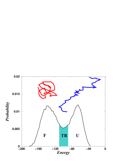
FIG. 1.: The probability distribution of the energy states $E$ of the 46-mer maintained at the folding transition temperature $T_{f}=1.44$. The bimodal distribution indicates the presence of two dominant states: the folded (region $F$) and the unfolded (region $U$) states. The transition state ensemble belongs to region TR of the histogram $\{-110<E<-90\}$. The insets show typical conformations in the folded and unfolded regions.

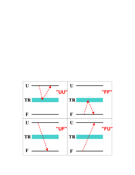
FIG. 2.: The schematic definition of the four types of conformations: FF, UU, UF, and FU.

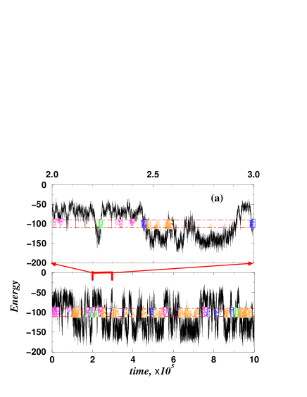
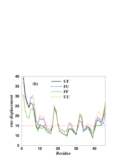
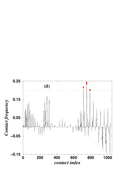
FIG. 3.: (a) The time evolution of the energy $E$ of the 46-mer maintained at the folding temperature $T_{f}=1.44$. We focus on region TR: $\{-110<E<-90\}$, which is denoted by two red dash-dotted lines. The triangles with arrows pointing up, down, left and right denote the conformations FF, UU, UF and FU. The upper figure magnifies the region $2\cdot 10^{5}\leq t\leq 3\cdot 10^{5}$. (b) The average rms displacement of each residue from its native state for each of the four types of TR conformations: FF, UU, UF and FU. Note that there is a pronounced difference in rms displacement of the residues from their native state in the vicinity of the residues 10 and 40. The red dash-dotted line indicates the breaking point of the native contacts, i. e. when the rms displacement $\sigma$ is approximately the size of the average relative distance between pairs of residues, i. e. $\sigma=(a_{0}+a_{1})/2\approx 15$ (see “Methods” section for the definition of $a_{0}$ and $a_{1}$). (c) The contact map of the model protein. The darker the shade of grey, the larger is the frequency of a contact. Above the diagonal of the square matrix shows the native contacts (see “Methods” section) of the FF conformations (if the native contact frequency is larger than 0.2). Below the diagonal of the square matrix shows the difference between the frequencies of the native contacts in FF and UU conformations (if this difference is larger than 0.2). Five contacts that persist in the FF conformations — $(11,39)$, $(10,40)$, $(11,40)$, $(10,41)$, and $(11,41)$ — are marked by crosses. The figure shows that identification of the protein folding nucleus is facilitated by the method used to construct the region of the matrix below the diagonal. (d) The contact frequency difference of the FF conformations versus UU conformations plotted versus the contact index $k=i(i-1)/2+j$, where $0\leq j<i=1,2,\dots 45$. The dashed-dotted line indicates the threshold value for the frequency differences. The circles indicate the contacts whose frequency differences are larger than the threshold. (Due to the scale used, only four contacts can be seen in the figure.)

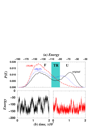
FIG. 4.: (a) The probability distribution of the energy states $E$ of the: (i) original 46-mer (at $T_{f}=1.44$), (ii) 46-mer (at $T=1.46$) with a fixed contact belonging to the protein folding nucleus, $(10,40)$, and (iii) 46-mer (at $T=1.46$) with fixed randomly-chosen control contact $(19,37)$, which does not belong to the protein folding nucleus. Note that the probability of the unfolded state of the 46-mer with a fixed contact belonging to the protein folding nucleus, is suppressed compared to that of the original 46-mer. (b) The time evolution of the energy $E$ of (i) original (left) and (ii) fixed $(10,40)$ contact (right). Case (iii) fixed $(19,37)$ contact is similar to (i), so we do not show it. For case (i), the fluctuations are mostly between two extreme values of energy, corresponding to the folded and unfolded states. In contrast, for case (ii), the fluctuations are mostly around one energy value, corresponding to the folded state.

REFERENCES

- [1] Jackson, S. Folding & Design, 3, R81–R91 (1998).
- [2] Karpov, V. G. & Oxtoby, D. W. Phys. Rev. B, 54, 9734–9745 (1996).
- [3] Lifshits, E. M. & Pitaevskii, L. P. Physical Kinetics (Pergamon, Oxford, New York; 1981).
- [4] Shakhnovich, E. I. Curr. Opin. Struct. Biol., 7, 29–40 (1997).
- [5] Fersht, A. Curr. Opin. Struct. Biol., 7, 10–14 (1997).
- [6] Pande, V. S., Grosberg, A. Yu., Rokshar, D. & Tanaka, T. Curr. Opin. Struct. Biol., 8, 68–79 (1998).
- [7] Abkevich, V. I., Gutin, A. M. & Shakhnovich, E. I. Biochemistry, 33, 10026–10036 (1994).
- [8] Shakhnovich, E. I. Folding & Design, 3, R108–R111 (1998).
- [9] Shakhnovich, E. I., Abkevich, V. I. & Ptitsyn, O. B. Nature, 379, 96–98 (1996)
- [10] Mirny, L., Abkevich, V. I. & Shakhnovich, E. I. Proc. Natl. Acad. Sci. USA, 95, 4976–4981 (1998).
- [11] Gutin, A. M., Abkevich, V. I. & Shakhnovich, E. I. Folding & Design, 3, 183–194 (1998).
- [12] Klimov, D. & Thirumalai, D. J. Mol. Biol., 282, 471–492 (1998).
- [13] Taketomi, H., Ueda, Y. & Gō , N. Int. J. Peptide Protein Res. 7, 445–459 (1975).
- [14] Gō , N. & Abe, H. Biopolymers 20, 991–1011 (1981).
- [15] Abe, H. & Gō , N. Biopolymers 20, 1013–1031 (1981).
- [16] Zhou, Y., Karplus, M., Wichert, J. M., & Hall, C. K. J. Chem. Phys., 107, 10691–10708 (1997).
- [17] Zhou, Y. & Karplus, M. Proc. Natl. Acad. Sci. USA, 94, 14429–14432 (1997).
- [18] Dokholyan, N. V., Buldyrev, S. V., Stanley, H. E. & Shakhnovich, E. I. Folding & Design, 3, 577–587 (1998).
- [19] Itzhaki, L., Otzen, D. & Fersht, A. J. Mol. Biol. , 254, 260–288 (1995).
- [20] Martinez, J., Pissabarro, T. & Serrano, L. Nature Struct. Biol., 5, 721–729 (1998).
- [21] Grantchanova V., Riddle, D., Santiago, J. & Baker, D. Nature Struct. Biol., 5, 714–720 (1998).
- [22] Perl, D., Welker, C., Schindler, T., Shroder, K., Marahiel, M., Jaenicke, R. & Schmid, F. X. Nature Struct. Biol., 5, 229–235 (1998).
- [23] Berriz, G. F., Gutin, A. M., & Shakhnovich, E. I. J. Chem. Phys. 106, 9276–9285 (1997).
- [24] Shakhnovich, E. I. & Gutin, A. M. Proc. Natl. Acad. Sci. USA 90, 7195–7199 (1993).
- [25] Abkevich, V. I., Gutin, A. M., & Shakhnovich, E. I. Folding & Design 1, 221–230 (1996).