Quantitative study of laterally inhomogeneous wetting films

Abstract

Based on a microscopic density functional theory we calculate the internal structure of the three-phase contact line between liquid, vapor, and a confining wall as well as the morphology of liquid wetting films on a substrate exhibiting a chemical step. We present a refined numerical analysis of the nonlocal density functional which describes the interface morphologies and the corresponding line tensions. These results are compared with those predicted by a more simple phenomenological interface displacement model. Except for the case that the interface exhibits large curvatures, we find that the interface displacement model provides a quantitatively reliable description of the interfacial structures.

I Introduction

The formation of a homogeneous wetting film of phase $\beta$ with thickness $l_{0}$ at the planar $\alpha$-$\gamma$ interface between two coexisting phases $\alpha$ and $\gamma$ is governed by the interplay of the surface tensions $\sigma_{\alpha\beta}$, $\sigma_{\beta\gamma}$, and $\sigma_{\alpha\gamma}$ [1, 2, 3, 4]. In the standard case $\beta$ and $\gamma$ are the liquid and vapor phases, respectively, of a simple fluid and $\alpha$ represents a substrate acting as an inert spectator phase. The translational invariance of these systems in the lateral directions can be broken either by opposing boundary conditions or by geometric or chemical heterogeneities within the confining medium $\alpha$. Whereas the first mechanism can always be applied, irrespective of the nature of the phase $\alpha$, the latter two mechanisms require a solid phase $\alpha$ which can permanently sustain well-defined lateral structures.

As a prerequisite for the possibility to impose opposing boundary conditions in lateral directions the thermodynamic state of the system has to be chosen such that the two phases $\beta$ and $\gamma$ are in thermal equilibrium. In that case the system can be arranged such that on its left end the substrate $\alpha$ is exposed to the vapor phase in the bulk whereas on its right end the substrate is exposed to the coexisting liquid phase in the bulk. This arrangement leads to the formation of a liquid-vapor interface intersecting the substrate at a three-phase contact line with the contact angle $\theta=\arccos((\sigma_{wg}-\sigma_{wl})/\sigma_{lg})$ (see Fig. 1). The free energy of this configuration decomposes into the volume contributions corresponding to the gas and liquid phases, respectively, the surface tensions $\sigma_{wg}$, $\sigma_{wl}$, and $\sigma_{lg}$ associated with the corresponding half-planes of contact between these phases, and the line tension $\tau$ associated with the presence of the three-phase contact line [1, 5, 6].

There have been numerous theoretical (see, e.g., Refs. [7, 8, 9, 10, 11, 12, 13, 14, 15]) and experimental (for a review see, e.g., Ref. [16]) efforts to determine the sign, magnitude, and temperature dependence of line tensions (see Refs. [17] and [18] for a recent summary of an extended list of additional references). In particular the singular behavior of the line tension upon approaching wetting transitions, i.e., for $\theta\to 0$ has been examined by using simple phenomenological interface displacement or square-gradient models [15, 19, 20, 21, 22]. Since the long-ranged, i.e., power-law decay of the dispersion forces acting in fluids is known to invalidate a gradient expansion for effective interface Hamiltonians [23, 24, 25, 26], in Ref. [17] the actual nonlocal interface Hamiltonian, as it is obtained from a microscopic nonlocal density functional theory, has been used to study the influence of dispersion forces on the line tension and on the intrinsic structure of the three-phase contact line. This study led to significant quantitative differences in comparison with the more simple interface displacement model.

Similar differences between the predictions of the nonlocal theory and its local approximation appeared [27] in the analysis of the morphology of a wetting film covering a planar substrate which consists of two adjacent halves composed of different materials and thus represents a chemical step (see Fig. 2). According to the results reported in Ref. [27] the nonlocal theory predicts a much broader transition region, within which the local film thickness $l(x)$ switches as function of the lateral coordinate $x$ between its asymptotic values $l_{\pm}=l(x\to\pm\infty)$, than the interface displacement model does.

The local interface displacement and square gradient theories relish popularity and are convenient for the description of thin fluid films on chemically or geometrically structured substrates (see, e.g., Refs. [28, 29, 30, 31, 32, 33, 34, 35, 36, 37, 38, 39]). In views of the aforementioned known limitations of the applicability of square gradient theories for systems governed by dispersion forces [23, 24, 25, 26] the objective of the present study is to pinpoint the reason for the reported large quantitative differences following from the local and the nonlocal approach. The common expectation is that the interface displacement model and the square gradient theory, although they are only approximations to the full nonlocal theory, turn out to yield nonetheless reliable results for most of the cases. The studies of the three-phase contact line (Sec. II) and of the adsorption on a chemical step (Sec. III) serve as testing grounds for the comparison between the local and the nonlocal theories. Our results are summarized in Sec. IV.

II Three-phase contact line

As stated in the Introduction we consider a simple fluid in a grand canonical ensemble described by the chemical potential $\mu$ and the temperature $T$. $\mu=\mu_{0}(T)$ is chosen such that in the bulk the fluid is at liquid-vapor coexistence. This allows one to maintain the configuration shown in Fig. 1 which is characterized by the number density $\rho(x,z)$ of the fluid particles. It interpolates smoothly between $\rho(x\to-\infty,z)=\rho_{-}(z)$, which corresponds to the wall-vapor interfacial profile, and $\rho(x\to\infty,z)=\rho_{+}(z)$, which describes the wall-liquid interfacial structure. The local position $l(x)$ of the liquid-vapor interface can be determined, e.g., as the isodensity contour line $\rho(x,z=l(x))=\frac{1}{2}(\rho_{l}+\rho_{g})$, where $\rho_{l}$ and $\rho_{g}$ are the bulk densities in the liquid and vapor phase, respectively. $l(x)$ asymptotically approaches the finite value $l_{0}(T)$ for $x\to-\infty$, which corresponds to the equilibrium wetting film thickness at the wall-vapor interface, and diverges linearly for $x\to\infty$ with a slope given by the contact angle (see Fig. 1).

A Density functional theory

Density functional theory has turned out to be a suitable theoretical description for spatially inhomogeneous fluids as considered here. We apply a simple [40] but nonetheless successful version which captures the essentials of wetting transitions [3]. Its grand canonical free energy functional reads

$$\Omega([\rho({\mathbf{r}})];T,\mu) = \int_{\Lambda}d^{3}rf_{HS}(\rho({\mathbf{r}}),T)+\int_{\Lambda}d^{3}r[V({\mathbf{r}})-\mu]\rho({\mathbf{r}})$$ (2)

$$+\frac{1}{2}\int_{\Lambda}d^{3}r\int_{\Lambda}d^{3}r^{\prime}\tilde{w}(|{\mathbf{r}}-{\mathbf{r}}^{\prime}|)\rho({\mathbf{r}})\rho({\mathbf{r}}^{\prime}).$$

$\Lambda$ is the finite volume filled by fluid within the half space $\Lambda_{+}=\{{\mathbf{r}}\in{\mathbb{R}}^{3}|z>0\}$. In the thermodynamic limit one has $\Lambda\to\Lambda_{+}$. The other half space $\{{\mathbf{r}}\in{\mathbb{R}}^{3}|z\leq 0\}$ is occupied by the substrate. The external potential $V({\mathbf{r}})$ describes the interaction of a fluid particle with the substrate:

$$V({\mathbf{r}})=V(z>0)=-\sum\limits_{i\geq 3}\frac{u_{i}}{z^{i}}.$$ (3)

Approximately $V(z)$ can be thought of as a laterally averaged pairwise sum of Lennard-Jones potentials

$$\phi_{w}(r)=4\epsilon_{w}\left[\left(\frac{\sigma_{w}}{r}\right)^{12}-\left(\frac{\sigma_{w}}{r}\right)^{6}\right]$$ (4)

between individual fluid and substrate particles.

$\tilde{w}(r)$ describes the attractive part of the pair potential between the fluid particles which is taken to be of Lennard-Jones type, i.e., $\phi_{f}(r)=4\epsilon_{f}[(\sigma_{f}/r)^{12}-(\sigma_{f}/r)^{6}]$. A division scheme like the Weeks-Chandler-Andersen (WCA) procedure [41] provides an attractive ($\phi_{att}$) and a repulsive part ($\phi_{rep}$) as suitable entries into the expression (2). We approximate the attractive part by the smooth function

$$\tilde{w}(r)=\frac{4w_{0}\sigma_{f}^{3}}{\pi^{2}}(r^{2}+\sigma_{f}^{2})^{-3}$$ (5)

where

$$w_{0}=\int_{{\mathbb{R}}^{3}}d^{3}r\,\tilde{w}(r)=\int_{{\mathbb{R}}^{3}}d^{3}r\,\phi_{att}(r)=-\frac{32}{9}\sqrt{2}\pi\epsilon_{f}\sigma_{f}^{3}.$$ (6)

$\tilde{w}(r)$ exhibits the main feature of the attractive van der Waals interaction, namely the large-distance behavior $\tilde{w}(r)\sim r^{-6}$. Its amplitude is chosen such that the integrated strength of $\tilde{w}(r)$ is the same as the integrated strength of $\phi_{att}$ as constructed from the WCA procedure. The repulsive part $\phi_{rep}(r)=\Theta(2^{1/6}\sigma_{f}-r)(\phi_{f}(r)+\epsilon_{f})$ (with the Heaviside step function $\Theta$) of the pair interaction gives rise to a reference free energy $f_{HS}(\rho,T)$ of a hard sphere fluid, for which we adopt the Carnahan-Starling approximation [42]:

$$f_{HS}(\rho,T)=k_{B}T\rho\left(\ln(\rho\lambda^{3})-1+\frac{4\eta-3\eta^{2}}{(1-\eta)^{2}}\right),$$ (7)

with the thermal de Broglie wavelength $\lambda$, the dimensionless packing fraction $\eta=\frac{\pi}{6}\rho(d(T))^{3}$, and the effective hard sphere diameter

$$d(T)=\int\limits_{0}^{2^{1/6}\sigma_{f}}dr\,\left\{1-\exp\left(-\frac{\phi_{rep}(r)}{k_{B}T}\right)\right\}.$$ (8)

In Eq. (2) the reference free energy is evaluated in a local density approximation and therefore it does not properly take into account the details of the packing effects near the wall. If one would be interested in these aspects, more sophisticated density functional theories have to be applied. Due to the last term in Eq. (2) the present density functional is a nonlocal expression. The bulk phase diagram, i.e., the values for the bulk particle densities $\rho_{l}(T,\mu)$ and $\rho_{g}(T,\mu)$ can be calculated by minimizing the bulk free energy density

$$\Omega_{b}(\rho,T,\mu)=f_{HS}(\rho,T)+\frac{1}{2}w_{0}\rho^{2}-\mu\rho$$ (9)

with respect to $\rho$, where $w_{0}$ is defined in Eq. (6). Equation (9) follows from inserting the homogeneous bulk density into Eq. (2). At two-phase coexistence one has

$$\left.\frac{\partial\Omega_{b}}{\partial\rho}\right|_{\rho=\rho_{g}}=\left.\frac{\partial\Omega_{b}}{\partial\rho}\right|_{\rho=\rho_{l}}=0\quad\mbox{and}\quad\Omega_{b}(\rho_{g})=\Omega_{b}(\rho_{l}).$$ (10)

With the bulk properties fixed the functional expression (2) can now be used to analyze the morphology and the line tension of a three-phase contact line. In spite of the relative simplicity of the expressions in Eq. (2) its full minimization with respect to $\rho(x,z)$ for the boundary conditions described in Fig. 1 represents a big numerical challenge. Since we are mainly interested in the local interface position we refrain from seeking this full solution. Instead we restrict the space of possible density distributions to a subspace of piecewise constant densities (see Fig. 3). Within this approximation at the position of the liquid-vapor interface $z=l(x)$ the density varies steplike between the bulk values determined by Eq. (9). Moreover, with $\rho(x,z<d_{w})=0$ (see Fig. 3) we take into account that there is an excluded volume near the substrate surface induced by the repulsive part of the substrate potential. Approximately one has $d_{w}=\frac{1}{2}(\sigma_{f}+\sigma_{w})$. Thus the analysis of the grand canonical functional amounts to inserting the steplike density distribution (“sharp-kink approximation”)

$$\hat{\rho}(x,z)=\Theta(z-d_{w})\{\rho_{l}\Theta(l(x)-z)+\rho_{g}\Theta(z-l(x))\}$$ (11)

into the functional (2), with $l(|x|\to\infty)$ asymptotically approaching the function

$$a(x)=l_{0}\Theta(-x)+(l_{0}+x\,\tan\theta)\Theta(x);$$ (12)

$\theta$ is the contact angle (see Fig. 1).

With this ansatz the grand canonical free energy functional can be systematically decomposed into bulk, surface, and line contributions. The decomposition is carried out for a finite system, and in a second step the thermodynamic limit is performed. This lengthy calculation is carried out in detail in Ref. [17]. Here we quote only the main results. There are artificial surface and line contributions which stem from truncating the system at finite distances before considering the thermodynamic limit; we omit them here. One obtains the following expression for $\Omega[\hat{\rho}]$:

$$\Omega[\hat{\rho}(x,z)] = \Lambda^{(l)}(\theta)\,\Omega_{b}(\rho_{l})+\Lambda^{(g)}(\theta)\,\Omega_{b}(\rho_{g})$$ (14)

$$+A\,\Omega_{s}(l_{0},\theta)+L_{y}\,\Omega_{l}[l(x)],$$

with the volumes $\Lambda^{(l)}=\frac{1}{4}L_{x}L_{y}\bar{L}(\theta)$ and $\Lambda^{(g)}=\frac{3}{4}L_{x}L_{y}\bar{L}(\theta)$, where $\bar{L}(\theta)=L_{z}-l_{0}=\frac{1}{2}L_{x}\tan(\theta)$, and the surface area $A=L_{x}L_{y}$ (see Fig. 1). The first two terms in Eq. (14) describe the bulk free energies of the liquid and vapor phases, with the bulk free energy density $\Omega_{b}(\rho_{\gamma})$ given by Eq. (9). The surface contribution $\Omega_{s}(l_{0},\theta)$ consists of the following terms:

$$\Omega_{s}(l_{0},\theta)=l_{0}\Omega_{b}(\rho_{l})+\sigma_{wl}+\frac{1}{2}\sigma_{lg}+\frac{1}{2\cos(\theta)}\sigma_{lg}+\frac{1}{2}\omega(l_{0})$$ (15)

where $\sigma_{wl}$ and $\sigma_{lg}$ are the wall-liquid and liquid-vapor surface tension, respectively. This expression corresponds to that for thin liquidlike wetting films adsorbed on homogeneous and planar substrates as obtained by the same approach [3]. In this context it is shown that the equilibrium thickness $l_{0}$ of the liquidlike film minimizes the effective interface potential

$$\omega(l)=\Delta\rho\left(\rho_{l}\int\limits_{l-d_{w}}^{\infty}dz\,t(z)-\int\limits_{l}^{\infty}dz\,V(z)\right)=\sum\limits_{i\geq 2}\frac{a_{i}}{l^{i}},\quad l\gg d_{w}.$$ (16)

$a_{2}$ is known as the Hamaker constant. The interaction potential $t(z)$ of a fluid particle with a half space occupied by fluid particles is given by

$$t(z)=\int\limits_{z}^{\infty}dz^{\prime}\int_{{\mathbb{R}}^{2}}d^{2}r_{\parallel}\tilde{w}(\sqrt{r_{\parallel}^{2}+z^{\prime 2}}).$$ (17)

The properties of the effective interface potential determine the character of the different wetting transitions. The contact angle $\theta$ follows from Young’s equation:

$$\cos\theta=\frac{\sigma_{wg}-\sigma_{wl}}{\sigma_{lg}}=1+\frac{\omega(l_{0})}{\sigma_{lg}}$$ (18)

with the liquid-vapor surface tension given within sharp-kink approximation by

$$\sigma_{lg}=-\frac{1}{2}(\Delta\rho)^{2}\int\limits_{0}^{\infty}dz\,t(z).$$ (19)

The line contribution can be split up into one term independent of $l(x)$ and one functionally depending on $l(x)$:

$$\Omega_{l}[l(x)]=\tau_{a}(l_{0},\theta)+\tau_{l}[l(x)]$$ (20)

with

$$\tau_{a}(l_{0},\theta) = \frac{w_{0}}{4\pi}(\Delta\rho)^{2}\left(1-\frac{\theta}{\tan\theta}\right)+\frac{\Delta\rho}{\tan\theta}\left[\left(-\frac{w_{0}}{2\pi}\right)\rho_{l}\right.$$ (22)

$$\left.\times\left\{[(l_{0}-d_{w})^{2}+\sigma_{f}]\left(-\frac{\pi}{2}+\arctan(l_{0}-d_{w})\right)+l_{0}-d_{w}\right\}+\sum\limits_{i\geq 1}\frac{1}{i(i+1)}\frac{u_{i+2}}{l_{0}^{i}}\right]$$

and

$$\tau_{l}[l(x)]=\tau_{\omega}[l(x)]+\tau_{i}[l(x)]$$ (23)

where the first term is given by an integral over the effective interface potential:

$$\tau_{\omega}[l(x)] = -\Delta\rho\left\{\rho_{l}\int\limits_{-\infty}^{\infty}dx\int\limits_{a(x)}^{l(x)}dz\,(\rho_{l}t(z-d_{w})-V(z))\right\}$$ (24)

$$= \int\limits_{-\infty}^{\infty}dx\,\{\omega(l(x))-\omega(a(x))\}$$ (25)

with $\omega(l)$ given by Eq. (16). The expression

$$\tau_{i}[l(x)] = \frac{1}{2}(\Delta\rho)^{2}\left\{\int\limits_{-\infty}^{\infty}dx\int\limits_{-\infty}^{\infty}dx^{\prime}\int\limits_{a(x)}^{l(x)}dz\int\limits_{-\infty}^{a(x^{\prime})}dz^{\prime}\,\bar{w}(|x-x^{\prime}|,|z-z^{\prime}|)\right.$$ (27)

$$-\left.\int\limits_{-\infty}^{\infty}dx\int\limits_{-\infty}^{\infty}dx^{\prime}\int\limits_{a(x)}^{l(x)}dz\int\limits_{l(x^{\prime})}^{\infty}dz^{\prime}\,\bar{w}(|x-x^{\prime}|,|z-z^{\prime}|)\right\}$$

describes the free energy contribution from the liquid-vapor interface and is a nonlocal functional of $l(x)$. In Eq. (27) $\bar{w}$ is an integral over the attractive fluid-fluid interaction

$$\bar{w}(x,z)=\int\limits_{-\infty}^{\infty}dy\,\tilde{w}(\sqrt{x^{2}+y^{2}+z^{2}}).$$ (28)

The expansion of the integrand in Eq. (27) into a Taylor series with respect to $|x-x^{\prime}|$ yields the gradient expansion of the functional expression, with the leading term

$$\tau_{i}^{(loc)}[l(x)]=\sigma_{lg}\int\limits_{-\infty}^{\infty}dx\left\{\sqrt{1+\left(\frac{dl}{dx}\right)^{2}}-\sqrt{1+\left(\frac{da}{dx}\right)^{2}}\right\},$$ (29)

which is now a local functional of $l(x)$.

The line contribution (Eq. (20)) to the free energy is minimized by using either Eq. (27) or Eq. (29), respectively, yielding the equilibrium liquid-vapor interface $\bar{l}(x)$ and the corresponding line tension $\tau$ as the minimum value $\Omega_{l}[\bar{l}(x)]$. In the following the application of Eq. (27) will be called “nonlocal theory”, whereas Eq. (29) is used for the so-called “local theory”, also known as “interface displacement model”. The expression in Eq. (29) measures the variation of surface free energy due to the deformation of the liquid-vapor interface. Equations (20)–(24) and (29) provide a prescription of how to introduce the parameters serving for a microscopic description of the underlying molecular interactions into the more simple interface displacement model which is originally motivated by phenomenological, macroscopic considerations.

B Intrinsic structure of the contact line

First we analyze the shape of the interface within the local theory. Minimization of Eq. (20) by using the functional in Eq. (29) leads to solving the corresponding Euler-Lagrange equation (ELE) following from $\delta\Omega_{l}/\delta l(x)=0$:

$$\left.\frac{d\omega(l)}{dl}\right|_{l=l(x)}=-\Delta\rho[\rho_{l}\,t(l(x)-d_{w})-V(l(x))]=\frac{\sigma_{lg}l\,^{\prime\prime}(x)}{(1+(l^{\prime}(x))^{2})^{3/2}}=\sigma_{lg}K(x).$$ (30)

$K(x)$ is the curvature of the planar trajectory $(x,l(x))$, with its local radius of curvature – which is also one of the two principal radii of curvature of the surface $(x,y,z=l(x))$ – given by $R=1/K$. It is related to the mean curvature $H$ of the manifold $(x,y,z=l(x))$ by $H(x)=\frac{1}{2}K(x)$. Equation (30) relates the local curvature $K(x)$ to the derivative of the effective potential (Eq. (16)) exerted on the liquid-vapor interface. The equation is often referred to as “augmented Young-Laplace equation” [33]. This nonlinear ordinary differential equation can easily be solved using standard numerical tools, e.g., the algorithms from the Numerical Algorithm Group (NAG). We have used a Runge-Kutta algorithm with a prescribed starting point $(x_{0},l_{0})$ and an initial derivative $l_{0}^{\prime}$. If $l_{0}^{\prime}=0$, the solution is $l(x)=l_{0}=\mbox{const}$, which describes the thin wetting film of constant thickness on the homogeneous and planar substrate. If, however, a very small initial derivative, e.g., $l_{0}^{\prime}=10^{-8}$, is chosen, then the solution diverges for increasing values of the lateral coordinate $x$, asymptotically exhibiting the constant slope $\tan\theta$ for $|x|\to\infty$. The origin of the coordinate system is then shifted in lateral direction such that the position $x=0$ corresponds to the intersection of the asymptotes of $l(x)$.

Figure 4 shows liquid-vapor interfaces around a three-phase contact line for a system undergoing a first-order wetting transition. Figure 4(a) displays the temperature dependence of the profiles $l(x)$, whereas Fig. 4(b) presents the deviation of the profiles from the asymptotes, i.e., $\delta l(x)\equiv l(x)-a(x)$. Apart from a different choice of interaction parameters and thus a different wetting transition temperature, these results are in agreement with those obtained in Ref. [17]. One of the main features in case of a first-order wetting transition is that $l(x\to\infty)$ approaches its asymptote from below ($\delta l(x>0)<0)$, whereas $l(x\to-\infty)$ approaches its asymptote from above ($\delta l(x<0)>0)$ (see also Ref. [20]). A more detailed discussion of the interface morphology is given in Ref. [17].

Within the nonlocal theory the ELE is the nonlocal integral equation

$$-\Delta\rho[\rho_{l}\,t(l(x)-d_{w})-V(l(x))]=-(\Delta\rho)^{2}\int\limits_{-\infty}^{\infty}dx^{\prime}\int\limits_{0}^{l(x^{\prime})-l(x)}dz^{\prime}\,\bar{w}(|x-x^{\prime}|,|z^{\prime}|),$$ (31)

i.e., the right-hand side of the local differential ELE (30) is replaced by an integral expression. In Ref. [17] the interface profiles within the nonlocal theory have been obtained from a numerical solution of the ELE (31). The insertion of the discretization $(x_{i},l_{i}=l(x_{i}))$ of the function $l(x)$ on a lattice with $N$ mesh points into Eq. (31) yields a set of $N$ coupled equations for the values $l_{i}$ which can be solved using standard numerical tools. This in itself is already a demanding task compared to the relatively easy numerical solution of the local ELE (30). But moreover the solution distinctly depends on the number of mesh points $N$, a fact that due to low computer power has not been revealed in Ref. [17]. An enhancement of $N$ such that the numerical resolution is satisfactory would require large computer memory and a very long time of computation. For this reason we numerically minimize the functional $\Omega_{l}^{(nloc)}[l(x)]$ itself, i.e., Eq. (20) with the nonlocal expression (27) for $\tau_{i}[l(x)]$, instead of solving the ELE. To this end the interface is also discretized $(x_{i},l_{i}=l(x_{i}))$ with a linear interpolation between the mesh points. The $z$ integration in Eq. (24) and the $z$ and $z^{\prime}$ integrations in Eq. (27) can be carried out analytically. With the remaining integrations performed numerically, the discretization procedure yields a function $\Omega_{l}(\{l_{i}\})$ which is minimized with respect to the $N$ variables $l_{i}$ using a particulary suitable algorithm from the NAG routine library. The price of a significant increase of the numerical effort, which is required by this approach as opposed to the seemingly easier way of solving Eq. (31) directly, is justified by the fact that the solution does not depend sensitively on the choice of the mesh size $\delta x=x_{i+1}-x_{i}$, as it does for the ELE (31). A repetition of the numerical minimization using a mesh with a larger number of points $N$ yields an identical result, which corroborates the reliability of the minimization procedure. Moreover, our results are in accordance with those obtained for geometrically structured, wegde-shaped systems which also indicate that interface profiles obtained from the local and the nonlocal theory differ only slightly [43].

The same minimization procedure can be applied to check the accuracy of the calculation of interface profiles within the local theory. As expected, the minimization of the expression (20) using the local functional Eq. (29) yields results identical to those obtained from the solution of the differential equation (30) whose numerical solutions do not depend on the number of mesh points.

For the same system as discussed in Fig. 4, Fig. 5 displays typical examples for the difference between the predictions obtained from the local and the nonlocal theory in terms of the deviation from the asymptotes $\delta l(x)$. Figure 6 shows the curvature $K(x)$ of the respective interfaces. $K(x)$ is slightly underestimated within the local theory. These figures clearly demonstrate that the obvious differences between the predictions of both theories are small and confined to those regions where $K(x)$ is largest. Significant deviations of the nonlocal predictions from the local ones only occur at sections of the interface where the radius of curvature $1/K(x)$ is less than $10\sigma_{f}$. This corrects the nonlocal results obtained in Ref. [17] from solving the ELE. Our refined numerical analysis shows that the differences are largest for high values of contact angle, i.e., for temperatures far below the wetting temperature. Upon approaching the wetting transition the contact angle and the curvature of the interface decrease, and the difference between the local and the nonlocal predictions becomes smaller.

Figure 7 displays liquid-vapor interfaces calculated within the local theory for a system which exhibits a critical wetting transition at $T_{w}^{*}=1.2$. In the case of critical wetting $l(x)$ approaches the asympotes from above both for $x\to\infty$ and for $x\to-\infty$, i.e., $\delta l(x)$ is always positive. If the system undergoes a critical wetting transition, the contact angles are rather small, and the interface profile exhibits very small local curvatures (see Fig. 7) and an extremely broad transition region (which is the interval where the deviation of $l(x)$ from its asymptotes is larger than a certain prescribed value).

In the case of a critical wetting transition it is presently impossible to perform a full numerical minimization of $\Omega_{l}^{(nloc)}$: due to the huge required system sizes over which the numerical integrations in Eqs. (24) and (27) have to be performed the available computer resources are by far exceeded. However, for a given equilibrium profile $\bar{l}(x)$ calculated within the local theory the relative difference $(\hat{\Omega}_{l}^{(nloc)}-\Omega_{l}^{(loc)})/\Omega_{l}^{(loc)}$, with $\hat{\Omega}_{l}^{(nloc)}$ evaluated for $\bar{l}(x)$, is of the order of $10^{-3}$. Therefore in the case of critical wetting we expect the difference between the interface profiles (as well as the line tensions) calculated within the local and the nonlocal theory to be negligibly small.

C Line tension

The line tension $\tau$ corresponding to the equilibrium liquid-vapor interface profile follows from Eqs. (20)-(29):

$$\tau^{((n)loc)}=\min_{\{l(x)\}}\Omega_{l}^{((n)loc)}[l(x)]=\Omega_{l}^{((n)loc)}[\bar{l}(x)].$$ (32)

Within the local theory $\tau^{(loc)}$ is obtained by inserting the solution $\bar{l}(x)$ of the ELE into $\Omega_{l}^{(loc)}$; within the nonlocal theory $\tau^{(nloc)}$ immediately follows from the minimization procedure itself.

Figure 8 shows the results for $\tau^{(loc)}$ and $\tau^{(nloc)}$ for the system undergoing a first-order wetting transition at $T_{w}^{*}=1.102$ (compare Figs. 4-6). Due to the large numerical effort only a few results have been obtained in the nonlocal theory. The data indicate that the difference $\tau^{(nloc)}-\tau^{(loc)}$ is rather small and vanishes upon approaching the wetting transition. A thorough discussion of the different contributions to the line tension is presented in Ref. [17], including a comparison with the singular behavior predicted by Indekeu [19, 20]. The results obtained in Ref. [17] for the local theory are still valid; therefore we can refrain from a further discussion here. We only show in Fig. 9 the temperature behavior of the two contributions $\tau_{\omega}$ and $\tau_{i}$ (Eqs. (23)-(29)) to the line tension $\tau$, as derived within local and nonlocal theory. The difference $\tau_{i}^{(nloc)}-\tau_{i}^{(loc)}$ is about twice the difference $\tau_{\omega}^{(nloc)}-\tau_{\omega}^{(loc)}$, and both vanish for $T\to T_{w}$.

III Adsorption on a chemical step

A Model and density functional theory

The study of the system shown in Fig. 2 is a first step towards the understanding of wetting on chemically heterogeneous surfaces [27]. In this case the translational symmetry in lateral directions is broken by the variation of the substrate potential in $x$ direction (Fig. 2). We describe the fluid in the half space $\{{\mathbf{r}}\in{\mathbb{R}}^{3}|z>0\}$ as in Sec. II (Eq. (2)). The only difference is that the substrate potential $V(z)$ in Eq. (3) is replaced by $V(x,z)$. As boundary condition one has $\rho(x,z\to\infty)=\rho_{g}$ for all $x$, including $|x|\to\infty$. To be specific we assume that the substrate potential is the pairwise superposition of Lennard-Jones pair potentials between the fluid and substrate particles,

$$\phi_{\pm}(r)=4\epsilon_{\pm}\left[\left(\frac{\sigma_{\pm}}{r}\right)^{12}-\left(\frac{\sigma_{\pm}}{r}\right)^{6}\right],$$ (33)

where the $+$ and $-$ signs stand for interaction of a fluid particle with the different species occupying the quarter spaces $w_{+}=\{{\mathbf{r}}\in{\mathbb{R}}^{3}|x>0,z<0\}$ and $w_{-}=\{{\mathbf{r}}\in{\mathbb{R}}^{3}|x<0,z<0\}$, respectively. This superposition yields [27]

$$V_{att}(x,z) = -\frac{u_{3}^{+}+u_{3}^{-}}{2}\frac{1}{z^{3}}+\frac{u_{3}^{+}-u_{3}^{-}}{2}\left(\frac{1}{x^{3}}-\left(\frac{r}{xz}\right)^{3}+\frac{3}{2}\frac{1}{xzr}\right)$$ (36)

$$-\frac{u_{4,z}^{+}+u_{4,z}^{-}}{2}\frac{1}{z^{4}}-\frac{u_{4,z}^{+}-u_{4,z}^{-}}{2}\left(\frac{x}{z^{4}r}+\frac{1}{2}\frac{x}{z^{2}r^{3}}\right)$$

$$+\frac{u_{4,x}^{+}-u_{4,x}^{-}}{2}\left(\frac{1}{x^{4}}-\left(\frac{z}{x^{4}r}+\frac{1}{2}\frac{z}{x^{2}r^{3}}\right)\right)+{\mathcal{O}}(x^{-m}z^{-n},\quad m+n\geq 5)$$

for the attractive part of the substrate potential, where $r\equiv r(x,z)=\sqrt{x^{2}+z^{2}}$. The coefficients $u_{3}^{\pm}$, $u_{4,z}^{\pm}$, and $u_{4,x}^{\pm}$ are functions of the interaction potential parameters $\epsilon_{\pm}$ and $\sigma_{\pm}$; $u_{3}^{\pm}$ and $u_{4,z}^{\pm}$ are the coefficients of the corresponding homogeneous, flat, semi-infinite substrate $w_{\pm}$ occupied by the species “$\pm$” with the substrate potential of a homogeneous substrate defined as in Eq. (3). For the repulsive contribution to the substrate potential we use the simple ansatz

$$V_{rep}(x,z)=\Theta(-x)\frac{u_{9}^{-}}{z^{9}}+\Theta(x)\frac{u_{9}^{+}}{z^{9}},$$ (37)

because the repulsive interaction of each half of the substrate decays rapidly.

This system has been studied in detail in Ref. [27]. As stated in the Introduction we revisit this problem in order to study the interface morphology with the refined numerical analysis described in Sec. II. Moreover, in Ref. [27] only the cases of critical and complete wetting have been covered. Here we also study a first-order wetting transition for which one can expect the largest differences between the local and the nonlocal approach (see Sec. II).

The behavior of the substrate potential $V(x,z)$ for large $|x|$ and $z$ fixed, i.e., far from the heterogeneity,

$$V(x\to\pm\infty,z)=-\frac{u_{3}^{\pm}}{z^{3}}-\frac{u_{4,z}^{\pm}}{z^{4}}+\frac{u_{9}^{\pm}}{z^{9}}\pm\frac{u_{3}^{+}-u_{3}^{-}}{|x|^{3}}+{\mathcal{O}}(|x|^{-4}),$$ (38)

causes the liquid-vapor interface to asymptotically approach the constant values $l(x\to\pm\infty)=l_{\pm}$ valid for the corresponding homogeneous substrate. Therefore it is appropriate to make the following sharp-kink ansatz for the particle density distribution (see Eq. (11)):

$$\hat{\rho}(x,z) = [\Theta(-x)\Theta(z-d_{w}^{-})+\Theta(x)\Theta(z-d_{w}^{+})]$$ (40)

$$\times[\rho_{l}\Theta(l(x)-z)+\rho_{g}\Theta(z-l(x))].$$

For this density distribution the grand canonical free energy functional decomposes into bulk, surface and line contributions such that the surface contribution describes the wetting of each single homogeneous, flat, semi-infinite substrate:

$$\Omega([\hat{\rho}(x,z)];T,\mu;[\tilde{w}],[V]) = \Lambda\,\Omega_{b}(\rho_{g},T,\mu)+A\,\Omega_{s}(l_{\pm};T,\mu;[\tilde{w}],[V])$$ (42)

$$+L_{y}\,\Omega_{l}([l(x)];T,\mu;[\tilde{w}],[V]),$$

where $\Omega_{b}$ is given by Eq. (9), $\Lambda=L_{x}L_{y}L_{z}$ is the volume filled with fluid, and $A=L_{x}L_{y}$ is the surface area of the substrate surface (see Fig. 2). Again artificial terms due to truncations are omitted.

$$\Omega_{s}(l_{\pm})=\frac{1}{2}(l_{+}+l_{-})\Delta\Omega_{b}+\sigma_{lg}+\frac{1}{2}(\sigma_{wl}(l_{+})+\sigma_{wl}(l_{-}))+\frac{1}{2}(\omega(l_{+})+\omega(l_{-}))$$ (43)

is the arithmetic mean of the surface free energy densities corresponding to wetting of the homogeneous substrates $w_{+}$ and $w_{-}$ by liquidlike layers of thickness $l_{+}$ and $l_{-}$, respectively. $\Delta\Omega_{b}=\Delta\rho\,\Delta\mu+{\mathcal{O}}((\Delta\mu)^{2})$ with $\Delta\rho=\rho_{l}-\rho_{g}$ measures the undersaturation if the liquid phase is not yet thermodynamically stable, i.e., if $\Delta\mu=\mu_{0}-\mu>0$. The line contribution $\Omega_{l}[l(x)]$ reads

$$\Omega_{l}[l(x)]=\tau_{wl}+\tau_{lg}+\tilde{\omega}[l(x)]$$ (44)

with

$$\tilde{\omega}[l(x)] = \Delta\Omega_{b}\int\limits_{-\infty}^{\infty}dx(l(x)-l_{\infty}(x))+\Delta\rho\,\rho_{l}\int\limits_{-\infty}^{\infty}dx\int\limits_{l(x)-d_{w}^{+}}^{l_{\infty}(x)-d_{w}^{+}}dz\,t(z)-\Delta\rho\int\limits_{-\infty}^{\infty}dx\int\limits_{l(x)}^{l_{\infty}(x)}dz\,V(x,z)$$ (47)

$$-\Delta\rho\,\rho_{l}\left(\int\limits_{-\infty}^{\infty}dx\int\limits_{l(x)-d_{w}^{+}}^{l_{\infty}(x)-d_{w}^{+}}dz\,\bar{t}(x,z)-\int\limits_{-\infty}^{\infty}dx\int\limits_{l(x)-d_{w}^{-}}^{l_{\infty}(x)-d_{w}^{-}}dz\,\bar{t}(x,z)\right)$$

$$-\frac{1}{2}(\Delta\rho)^{2}\int\limits_{-\infty}^{\infty}dx\int\limits_{-\infty}^{\infty}dx^{\prime}\int\limits_{0}^{\infty}dz\int\limits_{0}^{l(x)-l(x^{\prime})}dz^{\prime}\,\bar{w}(|x-x^{\prime}|,|z-z^{\prime}|)$$

where $l_{\infty}(x)\equiv\Theta(-x)l_{-}+\Theta(x)l_{+}$ and

$$\bar{t}(x,z)\equiv\int\limits_{x}^{\infty}dx^{\prime}\int\limits_{z}^{\infty}dz^{\prime}\,\bar{w}(x^{\prime},z^{\prime}).$$

The rather lengthy expressions $\tau_{wl}$ and $\tau_{lg}$ do not depend on the function $l(x)$ and are given in Ref. [27]. $\tilde{\omega}[l(x)]$ is a nonlocal functional which has to be minimized to yield the equilibrium profile $\bar{l}(x)$ and the line tension $\tau=\Omega_{l}[\bar{l}(x)]$.

The local approximation of the quadruple integral in $\tilde{\omega}[l(x)]$ – which describes the free energy contribution due to deformation of the liquid-vapor interface – is given by the local functional

$$-\frac{1}{2}(\Delta\rho)^{2} \int\limits_{-\infty}^{\infty}dx\int\limits_{-\infty}^{\infty}dx^{\prime}\int\limits_{0}^{\infty}dz\int\limits_{0}^{l(x)-l(x^{\prime})}dz^{\prime}\,\bar{w}(|x-x^{\prime}|,|z-z^{\prime}|)$$ (49)

$$\longrightarrow\quad\sigma_{lg}\int\limits_{-\infty}^{\infty}dx\left\{\sqrt{1+\left(\frac{dl}{dx}\right)^{2}}-1\right\}.$$

B Numerical results for the interface morphology

Within the local theory the interface morphology follows from the ELE

$$\Delta\Omega_{b}-\Delta\rho[\rho_{l}\,t(l(x)-d_{w})-V(x,l(x))]=\frac{\sigma_{lg}l\,^{\prime\prime}(x)}{(1+(l^{\prime}(x))^{2})^{3/2}}=\sigma_{lg}K(x).$$ (50)

Apart from the finite undersaturation $\Delta\Omega_{b}\geq 0$ and the different substrate potential the structure of this ELE is the same as in Eq. (30). For reasons of simplicity we assume that $d_{w}\equiv d_{w}^{+}=d_{w}^{-}$. Guided by the experience from Sec. II the equilibrium profile within the nonlocal theory is obtained by minimizing $\Omega_{l}$ (Eq. (44)) instead of solving the corresponding ELE as it has been done in Ref. [27]. Here we apply the same numerical procedures as in Sec. II.

Figure 10 displays interface profiles on a complete wetting path, i.e., along an isotherm $(T=\mbox{const},\Delta\mu\to 0)$; the system exhibits critical wetting transitions at $T_{w}^{*}=k_{B}T_{w}/\epsilon_{f}=1.2$ on the substrate $w_{-}$ and at $T_{w}^{*}=1.0$ on the substrate $w_{+}$, respectively. For the choice $T^{*}=1.1$ at coexistence the substrate $w_{+}$ is completely wet whereas $w_{-}$ is only partially wet. We find that the difference between the local and the nonlocal results for $l(x)$ as well as for the line tension $\tau$ is smaller than the numerical resolution and therefore not significant. The minimization procedure requires a large numerical effort and is only applied for values of $\mu$ not too close to coexistence $\mu=\mu_{0}$ such that the effective size of the system, which has to be treated numerically, is not too large.

For larger effective system sizes, i.e., close to coexistence $\Delta\mu=0$, we have to resort to an alternative procedure for evaluating the equilibrium interface profile $\bar{l}(x)$ within the nonlocal theory. The corresponding ELE

$$\Delta\Omega_{b}-\Delta\rho[\rho_{l}\,t(l(x)-d_{w})-V(x,l(x))]=-(\Delta\rho)^{2}\int\limits_{-\infty}^{\infty}dx^{\prime}\int\limits_{0}^{l(x^{\prime})-l(x)}dz^{\prime}\,\bar{w}(|x-x^{\prime}|,|z^{\prime}|)$$ (51)

(compare Eq. (31)) is solved numerically for a certain choice of thermodynamical parameters $(T,\mu)$. To this end the lateral extension of the system is truncated and $l(x)$ is discretized on a lattice with $N$ lattice points and a mesh size $\delta x$, yielding a set of $N$ coupled equations for the values $l_{i}=l(x_{i})$. These equations are solved using a suitable numerical algorithm. The solutions depend on the mesh size $\delta x$ in such a way that solutions $l(x;\delta x)$ for different $\delta x$ differ only with respect to a simple rescaling of the $x$ axis by a constant numerical factor. We note that this particular scaling behavior of the numerical solutions of the ELE only occurs in the present case of a substrate with a chemical step but not for the intrinsic structure of the contact lines investigated in Sec. II. Thus in the latter case this alternative approach is not applicable. The procedure of finding the correct solution is as follows. We calculate solutions of the ELE on lattices with different $\delta x$. A suitable length scale is defined which measures the typical width $\Delta$ on which the profile varies between its asymptotic values $l_{+}$ and $l_{-}$, e.g., the distance between the points where $l(x)$ deviates by $10\%$ from the asymptotes. As a function of $\delta x$ the width $\Delta$ asymptotically approaches a linear dependence $\Delta(\delta x\to 0)=A\,\delta x+B$ which can be extrapolated to $\delta x=0$. This yields a factor $\gamma_{0}=\Delta(\delta x=0)/\Delta(\delta x_{0})$ by which a certain solution $l(x;\delta x_{0})$ of the ELE has to be scaled in $x$ direction in order to find the limiting profile corresponding to an infinitely fine lattice (see Fig. 11). In order to test the reliability of this approach we have carried out the following additional cross-check: a solution $l(x;\delta x_{0})$ of the ELE obtained by using a mesh size $\delta x_{0}$ is scaled in $x$ direction by different factors, i.e., $x\mapsto\gamma\,x$; the correct scaling factor $\gamma_{0}$ is the one for which the line contribution to the free energy $\Omega_{l}[l(\gamma\,x;\delta x_{0})]$ is minimized. Both procedures are based on the assumption that the true solution differs from each of the numerically obtained solutions $l(x;\delta x)$ only by a simple rescaling of the $x$ axis. (For those systems, for which the full minimization and the solution of the ELE can be carried out both, this assumption has been verified.) Within the numerical accuracy the two methods give identical results for the scaling factor. Moreover, as expected the solution obtained by rescaling of the $x$ axis with this optimal factor is indistinguishable from the one predicted by the local theory.

Figure 12 shows interface profiles for a thermodynamic path along coexistence $(T\to T_{w},\Delta\mu=0)$. The system exhibits critical wetting at the same transition temperature $T_{w}^{*}=1.0$ for both substrates $w_{+}$ and $w_{-}$; the parameters of the substrate potential are chosen such that the asymptotic equilibrium film thicknesses $l_{+}$ and $l_{-}$ are different although the wetting transition temperatures are equal. Due to the broad crossover region these profiles have been obtained by using the scaling procedure as described for finding the minimum of $\Omega_{l}$. Also in this case the local and the nonlocal results are indistinguishable. Not only the profiles but also the line tensions obtained within the local and the nonlocal theory, respectively, are very close. The relative difference of the line tensions $(\tau^{(nloc)}-\tau^{(loc)})/\tau^{(loc)}$ is of the order of $10^{-4}$, both for complete as well as for critical wetting.

In Fig. 13 we present results for interface profiles for a system with very thin liquidlike wetting films. Both corresponding homogeneous substrates undergo first-order wetting transitions: $w_{+}$ at the temperature $T_{w}^{*}\approx 1.102$ and $w_{-}$ at $T_{w}^{*}\approx 1.314$; both wetting temperatures are above the temperatures considered here. In the previous examples the differences between the results obtained within the local and nonlocal theory are small. But here they are detectable since the interface curvatures are larger than in a system with thick wetting films as they occur for critical and complete wetting. The relative difference $(\tau^{(nloc)}-\tau^{(loc)})/\tau^{(loc)}$ is of the order of $10^{-2}$.

IV Summary

We have analyzed the morphology and the associated line tensions of liquidlike wetting films at a three-phase contact line (Fig. 1) and on a planar substrate across a chemical step (Fig. 2). By using refined numerical techniques we have compared quantitatively the predictions obtained within a local displacement model for the interface profile and within a nonlocal density functional theory. Based on general arguments [23, 24, 25, 26] the latter approach is the more accurate one. We have obtained the following main results:

1. Within the present mean-field theories the equilibrium interfacial profiles are determined as the minimum of the line contribution to the functional of the grand canonical free energy. These equilibrium profiles, within the sharp-kink approximation (Fig. 3), can be obtained either by an explicit minimization procedure or by solving the corresponding Euler-Lagrange equation for the minimum. Within the local theory both approaches are equally successful and robust. However, within the nonlocal theory in practical terms only the minimization procedure yields reliable access to the true minimum whereas solving the necessarily discretized version of the nonlocal Euler-Lagrange equation leaves one with a very slow convergence with respect to the mesh size of the discretization. This mesh size dependence of the solutions within the nonlocal theory was not revealed in Refs. [17] and [27] and led to a significant overestimation of the quantitative discrepancy between the predictions of the local and the nonlocal theory.

2. Concerning the intrinsic structure of the three-phase contact line the local and the nonlocal theory yield only slightly different interface morphologies (Figs. 4 and 5) and line tensions (Figs. 8 and 9) in the case of first-order wetting. In the case of critical wetting the two theories yield indistinguishable results (Fig. 7). For first-order wetting the deviations between the results obtained from the local and the nonlocal theories are confined to regions within which the radius of curvature of the interface profile is less than about 10 atomic diameters $\sigma_{f}$ of the fluid particles (Fig. 6). Upon approaching a first-order wetting transition the line tension $\tau$ of the three-phase contact line diverges logarithmically (Figs. 8 and 9). $\tau$ changes sign as a function of temperature and typically is of the order of $\epsilon_{f}/\sigma_{f}$ where $\epsilon_{f}$ is the depth of the interaction potential between the fluid particles.

3. Concerning the morphology of a wetting film on a planar substrate with a chemical step the results obtained from the local and the nonlocal theory for complete and critical wetting are indistinguishable (Figs. 10 and 12). Small differences appear only in the case of first-order wetting (Fig. 13).

Thus we conclude that the local interface displacement model yields quantitatively reliable results for the interface morphology and the line tension of laterally inhomogeneous wetting films. The more accurate nonlocal description is necessary only for cases in which the interface profiles exhibit large curvatures. Thus all results and discussions in Refs. [17] and [27] based on the local theory turn out to provide actually a quantitatively reliable description of the systems under consideration.

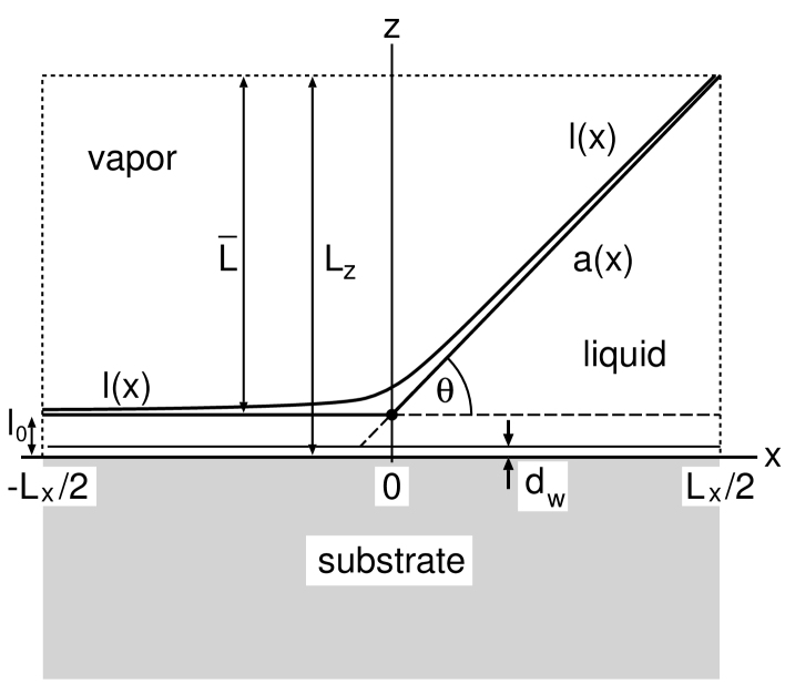
FIG. 1.: Shape $l(x)$ of the liquid-vapor interface near the three-phase contact line on a homogeneous, planar substrate whose surface is located at $z=0$. $l_{0}$ is the thickness of the microscopic liquid wetting film, $d_{w}$ denotes an excluded volume due to the repulsive part of the substrate potential. $a(x)$ is the asymptote $l(x)$ in the limit $|x|\to\infty$. The angle $\theta$ between $a(x>0)$ and the substrate surface is the contact angle given by Young’s law $\cos\theta=(\sigma_{wg}-\sigma_{wl})/\sigma_{lg}$. The intersection between the asymptotes $a(x<0)$ and $a(x>0)$ defines the position $x=0$. In order to facilitate the proper thermodynamic limit the system is truncated at $x=\pm L_{x}/2$ and $z=L_{z}$. The configuration is taken to be translationally invariant in the $y$ direction.

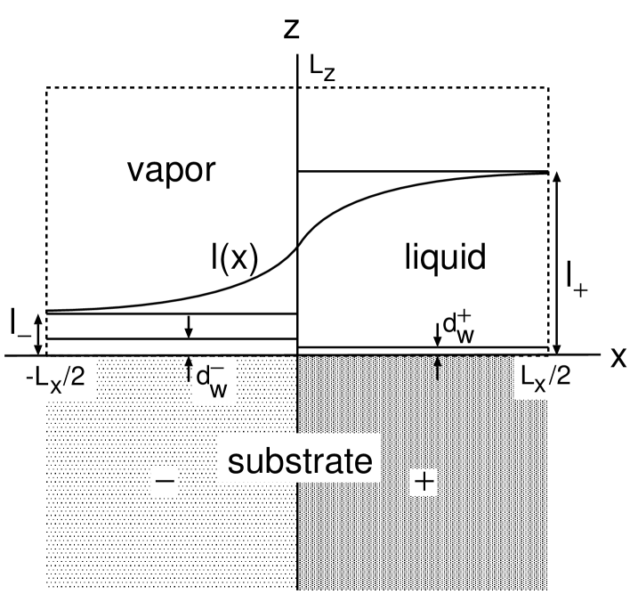
FIG. 2.: Morphology $l(x)$ of a wetting film which covers a planar substrate with surface $z=0$. The substrate consists of two halves meeting at $x=0$. The material filling the left (right) half favors a thin (thick) wetting film. $l_{\mp}=l(x\to\mp\infty)$ are the equilibrium film thicknesses of the corresponding homogeneous substrates, which are characterized also by different excluded volumes $d_{w}^{\mp}$. The system is translationally invariant in the $y$ direction. It is truncated at $z=L_{z}$ and $x=\mp L_{x}/2$ in order to facilitate the proper thermodynamic limit.

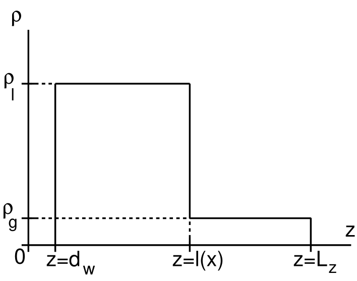
FIG. 3.: Sharp-kink approximation for the particle density distribution. At the position $z=l(x)$ of the liquid-vapor interface the particle density distribution varies steplike between the constant liquid ($\rho_{l}$) and the constant gas density ($\rho_{g}$). At $z=L_{z}$ the density is truncated in order to facilitate the thermodynamic limit. Moreover, the density vanishes for $z<d_{w}$ due to the repulsion between the fluid and the substrate particles.

FIG. 4.: Temperature dependence of the shape of the liquid-vapor interface calculated within the local theory for a system which exhibits a first-order wetting transition at $T_{w}^{*}=k_{B}T_{w}/\epsilon_{f}\approx 1.102$. The substrate potential parameters are $d_{w}=1.05\sigma_{f}$, $u_{3}=3.710\epsilon_{f}\sigma_{f}^{3}$, $u_{4}=5.566\epsilon_{f}\sigma_{f}^{4}$, and $u_{9}=0.876\epsilon_{f}\sigma_{f}^{9}$. In (a) the interface profiles $l(x)$ (full lines) and their asymptotes $a(x)$ (dashed lines) are shown, whereas (b) displays the deviation $\delta l(x)=l(x)-a(x)$ of $l(x)$ from its asymptotes. The corresponding contact angles are $\theta\approx 44.5^{\circ}$, $\theta\approx 36.9^{\circ}$, and $\theta\approx 26.6^{\circ}$ for $T^{*}=0.8$, $0.9$, and $1.0$, respectively. $l(x)$ approaches its asymptotes from above for $x\to-\infty$ and from below for $x\to\infty$. $l(x)$ closely follows the asymptotes for large values of the contact angle, i.e., for low temperatures.

FIG. 5.: Comparison between liquid-vapor interface profiles calculated within the local (dashed lines) and the nonlocal (full lines) theory for the same system as discussed in Fig. 4, in terms of the difference $\delta l(x)=l(x)-a(x)$ for $T^{*}=0.8$ (a) and $T^{*}=1.0$ (b). The difference between the local and the nonlocal results decreases upon approaching the wetting transition. The local theory slightly underestimates the local curvature $K(x)$.

FIG. 6.: Comparison between the curvatures $K(x)=l\,^{\prime\prime}(x)/(1+(l\,^{\prime}(x))^{2})^{3/2}$ of the liquid-vapor interface profiles as calculated within the local (dashed lines) and the nonlocal (full lines) theory for the same system as in Fig. 4. The parameters chosen for (a) and (b) are the same as for Figs. 5(a) and 5(b), respectively. Also for the curvature the difference between the local and the nonlocal results decreases upon approaching the wetting transition. The local theory slightly underestimates the curvature.

FIG. 7.: Liquid-vapor interfaces calculated within the local theory for a system which exhibits a critical wetting transition at $T_{w}^{*}=1.2$. Here the substrate potential parameters are $d_{w}=\sigma_{f}$, $u_{3}=1.683\epsilon_{f}\sigma_{f}^{3}$, $u_{4}=10.098\epsilon_{f}\sigma_{f}^{4}$, and $u_{9}=0.224\epsilon_{f}\sigma_{f}^{9}$. In (a) the interface profiles $l(x)$ (full lines) and their asymptotes $a(x)$ (dashed lines) are shown, whereas (b) displays the deviation $\delta l(x)=l(x)-a(x)$ of $l(x)$ from its asymptotes. The corresponding contact angles are $\theta\approx 0.31^{\circ}$, $\theta\approx 0.17^{\circ}$, and $\theta\approx 0.06^{\circ}$ for $T^{*}=1.14$, $1.16$, and $1.18$, respectively. $l(x)$ approaches its asymptotes from above both for $x\to-\infty$ and $x\to\infty$. In (c) the curvatures $K(x)$ are plotted. As compared to the system exhibiting a first-order wetting transition (see Figs. 4 – 6) $\delta l(x)$ and the radii of curvature $1/K(x)$ are extremely large . Due to numerical difficulties no data for the nonlocal theory are available for this system. However, since the interface curvature is several orders of magnitude smaller than in the system which displays a first-order wetting transition – with already small deviations of the local from the nonlocal theory – the difference between local and nonlocal results for the present system is expected to be indistinguishable on this scale.

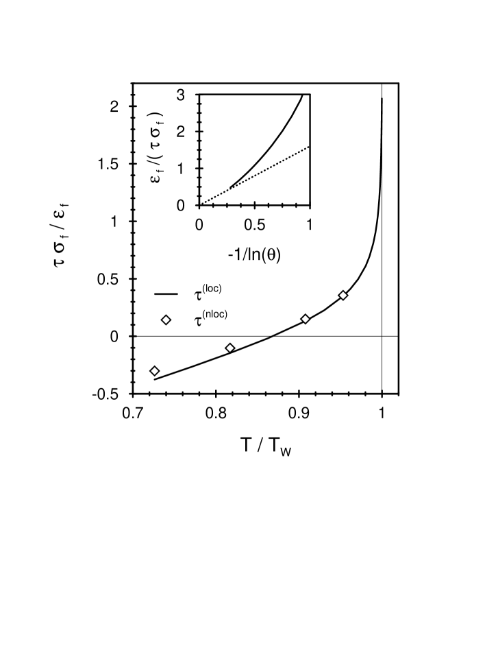
FIG. 8.: Line tensions as predicted by the local and the nonlocal theory for the same system as in Fig. 4. The transition temperature for first-order wetting is $T_{w}^{*}\approx 1.102$. The difference $\tau^{(nloc)}-\tau^{(loc)}$ vanishes upon approaching $T_{w}$. The singular behavior of the line tension can be derived analytically within the local theory; upon approaching the wetting transition $\tau$ diverges as $\tau(T\to T_{w})\sim\ln(\theta(T))$, as indicated in the inset. (The dotted line is the estimated extrapolation according to the logarithmic divergence.) We note that as function of temperature $\tau$ changes sign. Apart from the close vicinity of $T_{w}$ and its zero the absolute value of $\tau$ is of the order of $\epsilon_{f}/\sigma_{f}$.

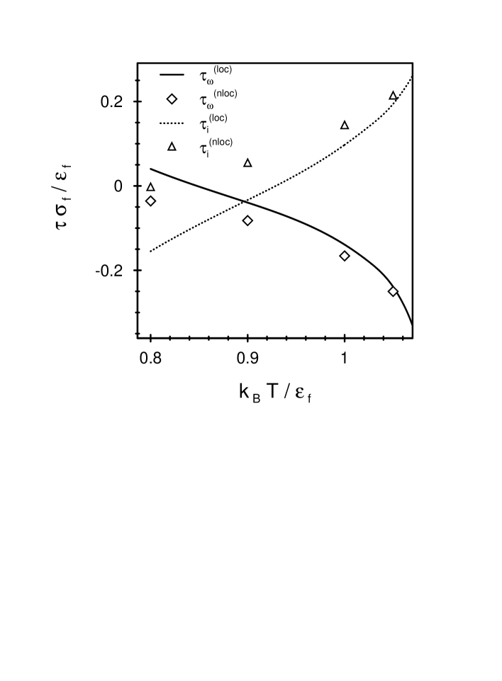
FIG. 9.: Temperature dependence of the contributions $\tau_{\omega}$ and $\tau_{i}$ (Eqs. (23)-(29)) to the line tensions $\tau^{(nloc)}$ and $\tau^{(loc)}$ for the same system as in Figs. 4 and 8. For $T\to T_{w}\approx 1.102\epsilon_{f}/k_{B}$ both $\tau_{\omega}^{(nloc)}-\tau_{\omega}^{(loc)}$ and $\tau_{i}^{(nloc)}-\tau_{i}^{(loc)}$ vanish. As already discussed in Ref. [17], the leading singular behaviors $\tau_{\omega}\sim-1/\theta$ and $\tau_{i}\sim 1/\theta$ for $\theta\to 0$, i.e., $T\to T_{w}$ compensate each other in $\tau=\tau_{\omega}+\tau_{i}$, leaving the residual singularity $\tau\sim-\ln(\theta)$.

FIG. 10.: Shape of the liquid-vapor interface on a planar substrate exhibiting a chemical step (see Fig. 2) within nonlocal and local theory along an isotherm $(T^{*}=1.1,\Delta\mu^{*}=\Delta\mu/\epsilon_{f}\to 0)$, i.e., for complete wetting. The parameters for the substrate potential are chosen such that both substrates individually exhibit critical wetting transitions, the substrate $w_{-}$ ($x<0$) at $T_{w}^{*}=1.2$ and the substrate $w_{+}$ ($x>0$) at $T_{w}^{*}=1.0$: $d_{w}^{+}=\sigma_{f}$, $u_{3}^{+}=2.079\epsilon_{f}\sigma_{f}^{3}$, $u_{4,z}^{+}=u_{4,x}^{+}=12.475\epsilon_{f}\sigma_{f}^{4}$, and $u_{9}^{+}=0.277\epsilon_{f}\sigma_{f}^{9}$, whereas the parameters $d_{w}^{-}$ and $u_{j}^{-}$ are chosen as in Fig. 7 with $u_{4,x}^{-}=u_{4,z}^{-}$. Therefore for this temperature at coexistence $\Delta\mu=0$ the substrate $w_{+}$ is wet whereas the substrate $w_{-}$ remains only partially wet so that $l(x\to\infty,\Delta\mu=0)=\infty$ and $l(x\to-\infty,\Delta\mu=0)<\infty$. The nonlocal result for $\Delta\mu=1.5\cdot 10^{-6}$ has been obtained by solving the discretized version of the ELE on lattices of different mesh size $\delta x$ and the application of a pointwise extrapolation scheme $\delta x\to 0$ as outlined in the main text. The other interfacial shapes calculated within the nonlocal theory result from a free numerical minimization of the line contribution to the free energy $\Omega_{l}^{(nloc)}[l(x)]$. The differences between the local and the nonlocal results are not visible on this scale. Therefore only one type of line is shown for each interfacial profile.

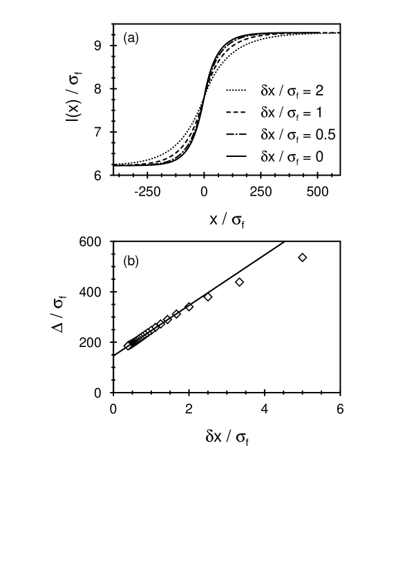
FIG. 11.: Dependence of the numerical solutions of the nonlocal ELE on the mesh size $\delta x$ for the same set of parameters as in Fig. 10 and for $\Delta\mu^{*}=10^{-3}$. (a) displays profiles obtained for different values of $\delta x$. As $\delta x$ is decreased, the distance $\Delta$ between the two points where $l(x)$ deviates from the asymptotes $l_{+}$ and $l_{-}$ by $10\%$ becomes smaller, as shown in (b). This dependence can be extrapolated to the limit $\delta x=0$, as indicated by the straight line in (b). Using the value of $\Delta$ from this extrapolation, the correct result in the limit of an infinitely fine lattice can be obtained along the lines discussed in the main text. This limiting profile is shown in (a) ($\delta x=0$); it turns out to be indistinguishable from both the local result and the result obtained by the full numerical minimization of $\Omega_{l}^{(nloc)}$ which can also be carried out for the present example.

FIG. 12.: Liquid-vapor interfaces on a planar substrate with a chemical step (see Fig. 2) as obtained within the nonlocal and the local theory. The parameters for the substrate potential are chosen such that both substrates exhibit critical wetting at the same transition temperature $T_{w}^{*}=1.0$. The parameters $d_{w}^{+}$ and $u_{j}^{+}$ are chosen as in Fig. 10, whereas $d_{w}^{-}=\sigma_{f}$, $u_{3}^{-}=u_{3}^{+}$, $u_{9}^{-}=u_{9}^{+}$, and $u_{4,z}^{+}=u_{4,x}^{+}=15.594\epsilon_{f}\sigma_{f}^{4}$. The profiles are calculated for different temperatures $T^{*}$ on a thermodynamic path along coexistence $\Delta\mu=0$. The nonlocal results for both temperatures have been obtained by applying the extrapolation scheme explained in the main text. On the present scale the local and nonlocal results are indistinguishable and therefore only one type of lines is shown.

FIG. 13.: Liquid-vapor interfaces on a substrate with a chemical step at $x=0$ (see Fig. 2) as obtained within the nonlocal and the local theory. The parameters for the substrate potential are chosen such that both substrates individually exhibit first-order wetting transitions, the substrate $w_{-}$ at $T_{w}^{*}\approx 1.314$ (with $d_{w}^{-}=\sigma_{f}$, $u_{3}^{-}=2.513\epsilon_{f}\sigma_{f}^{3}$, $u_{4,z}^{-}=u_{4,x}^{-}=3.770\epsilon_{f}\sigma_{f}^{4}$, and $u_{9}^{-}=0.335\epsilon_{f}\sigma_{f}^{9}$) and the substrate $w_{+}$ at $T_{w}^{*}\approx 1.102$ (with the parameters $d_{w}^{+}$ and $u_{j}^{+}$ as for Fig. 4 and $u_{4,x}^{+}=u_{4,z}^{+}$). The system is at coexistence $\Delta\mu=0$. Within the nonlocal and the local theory both profiles are obtained by a full numerical minimization of the line contribution to the free energy $\Omega_{l}^{((n)loc)}$. The differences between the local and the nonlocal results are very small but detectable. The relative difference in line tensions $(\tau^{(nloc)}-\tau^{(loc)})/\tau^{(loc)}$ is of the order of $10^{-2}$.

- [1] P. G. de Gennes, Rev. Mod. Phys. 57, 827 (1985).
- [2] D. E. Sullivan and M. M. Telo da Gama, in Fluid interfacial phenomena, edited by C. A. Croxton (Wiley, New York, 1986), p. 45.
- [3] S. Dietrich, in Phase Transitions and Critical Phenomena, edited by C. Domb and J. L. Lebowitz (Academic, London, 1988), Vol. 12, p. 1.
- [4] M. Schick, in Liquids at interfaces, Proceedings of the Les Houches Summer School Lectures, Session XLVIII, edited by J. Chavrolin, J. F. Joanny, and J. Zinn-Justin (Elsevier, Amsterdam, 1990), p. 415.
- [5] J. W. Gibbs, The collected works of J. Willard Gibbs (Yale University Press, London, 1957), p. 288.
- [6] J. S. Rowlinson and B. Widom, Molecular Theory of Capillarity (Clarendon, Oxford, 1982).
- [7] M. V. Berry, J. Phys. A 7, 231 (1974).
- [8] B. A. Pethica, J. Colloid Interface Sci. 62, 569 (1977).
- [9] R. E. Benner Jr., L. E. Scriven, and H. T. Davis, Faraday Symp. Chem. Soc. 16, 169 (1981).
- [10] P. Tarazona and G. Navascués, J. Chem. Phys. A 75, 3114 (1981).
- [11] B. V. Toshev, D. Platikanov, and A. Scheludko, Langmuir 4, 489 (1988).
- [12] C. Varea and A. Robledo, Physica A 183, 12 (1992).
- [13] I. Szleifer and B. Widom, Mol. Phys. 75, 925 (1992).
- [14] F. Bresme and N. Quirke, Phys. Rev. Lett. 80, 3791 (1998).
- [15] H. T. Dobbs, Katholieke Universiteit Leuven preprint, Belgium (1998).
- [16] J. Drelich, Colloids Surf. A 116, 43 (1996).
- [17] T. Getta and S. Dietrich, Phys. Rev. E 57, 655 (1998).
- [18] S. Dietrich, Fluids in contact with structured substrates, proceedings of the NATO-ASI on New approaches to old and new problems in liquid state theory: inhomogeneities and phase separation in simple, complex, and quantum fluids, held at Patti Marina, Italy, July 7-17, 1998, edited by C. Caccamo (Kluwer, Dordrecht, in press).
- [19] J. O. Indekeu, Physica A 183, 439 (1992).
- [20] J. O. Indekeu, Int. J. Mod. Phys. B 8, 309 (1994).
- [21] J. O. Indekeu and H. T. Dobbs, J. Phys. I (France) 4, 77 (1994).
- [22] J. O. Indekeu and A. Robledo, Phys. Rev. E 47, 4607 (1993).
- [23] S. Dietrich and M. Napiórkowski, Physica A 177, 437 (1992).
- [24] M. Napiórkowski and S. Dietrich, Z. Phys. B – Condens. Matter 89, 263 (1992).
- [25] M. Napiórkowski and S. Dietrich, Phys. Rev. E 47, 1836 (1993).
- [26] M. Napiórkowski and S. Dietrich, Z. Phys. B – Condens. Matter 97, 511 (1995).
- [27] W. Koch, S. Dietrich, and M. Napiórkowski, Phys. Rev. E 51, 3300 (1995).
- [28] M. W. Cole and E. Vittoratos, J. Low Temp. Phys. 22, 223 (1976).
- [29] E. Cheng and M. W. Cole, Phys. Rev. B 41, 9650 (1990).
- [30] M. Kardar and J. O. Indekeu, Europhys. Lett. 12, 161 (1990).
- [31] M. O. Robbins, D. Andelman, and J.-F. Joanny, Phys. Rev. A 43, 4344 (1991).
- [32] M. Napiórkowski, W. Koch, and S. Dietrich, Phys. Rev. A 45, 5760 (1992).
- [33] M. Kagan, W. V. Pinczewski, and P. E. Oren, J. Colloid Interf. Sci. 170, 426 (1995).
- [34] J. V. Andersen and H. J. Jensen, Phys. Rev. Lett. 80, 3555 (1998).
- [35] P. S. Swain and A. O. Parry, Eur. Phys. J. B 4, 459 (1998).
- [36] C. Rascón and A. O. Parry, Phys. Rev. Lett. 81, 1267 (1998).
- [37] C. J. Boulter, Phys. Rev. E 57, 2062 (1998).
- [38] A. L. Stella and G. Sartoni, Phys. Rev. E 58, 2979 (1998).
- [39] P. S. Swain and R. Lipowsky, Langmuir 14, 6772 (1998)
- [40] R. Evans, Adv. Phys. 28, 143 (1979).
- [41] J. D. Weeks, D. Chandler, and H. C. Andersen, J. Chem. Phys. 54, 5237 (1971); H. C. Andersen, J. D. Weeks, and D. Chandler, Phys. Rev. A 4, 1597 (1971).
- [42] N. F. Carnahan and K. E. Starling, J. Chem. Phys. 51, 635 (1969).
- [43] T. Boigs and S. Dietrich, unpublished.