Topological defects and the short-distance behavior of the structure factor in nematic liquid crystals

Abstract

The scattering of light at large wave-vector magnitudes $k$ in nematic systems containing topological defects is investigated theoretically. At large $k$ the structure factor $S(k)$ is dominated by power-law contributions originating from singular order-parameter variations associated with topological defects and from transverse thermal fluctuations of the nematic director. These defects (nematic disclinations and hedgehogs) lead to contributions of the form $\rho Ak^{-\xi}$ (“the Porod tail”), where $\rho$ is the number density of a given type of defect, $A$ is a dimensionless Porod amplitude, and $\xi$ is an integer-valued Porod exponent. The Porod amplitudes and exponents are calculated for all types of topologically stable defects occurring in uniaxial and biaxial nematics in two or three spatial dimensions. The range of wave-vectors in which the contributions to the scattering intensity due to defects dominate the contribution due to thermal fluctuations is estimated, and it is concluded that for experimentally accessible defect densities the range of observability of the Porod tail extends over one to three decades in scattering wave-vector magnitude $k$. Available experimental results on phase ordering in uniaxial nematics are analyzed, and applications of our results are suggested for light-scattering studies of other nematic systems containing numerous defects.

I Introduction

When a liquid crystalline material is brought from the isotropic phase to the nematic phase, the turbidity (i.e., the total intensity of scattered light) of the material increases by a factor of the order of $10^{6}$, and the sample appears cloudy [3]. In samples in which the nematic ordering is well aligned, this intense scattering is due predominantly to thermal fluctuations in the orientation of the nematic director, and has been extensively studied and reported in the literature [3, 4, 5, 6]. If, on the other hand, the sample is not well aligned and contains a large number of topological defects (disclinations, nematic hedgehogs, or surface defects), the turbidity becomes dominated by scattering from essentially static director inhomogeneities associated with these defects [6].

A particularly visible manifestation of defect-associated scattering is the so-called “Porod tail” contribution to the scattering intensity. For sufficiently large magnitudes $k$ of the scattering wave-vector ${\bf k}$, the scattered light intensity $I({\bf k})$ of a nematic system containing topological defects decays as a power law $k^{-\chi}$, where $\chi$ is an integer-valued exponent that depends on the dominant type of defect present in the system. Such behavior was confirmed and the values of $\chi$ have been discussed in both the experimental [7, 8] and the theoretical [9] literature on the kinetics of phase ordering of nematic systems containing numerous defects generated during a quench from the isotropic to the nematic phase. A full calculation of the form of the power-law tails associated with nematic defects, and an evaluation of the relative importance of these contributions compared to the $k^{-2}$ contribution associated with thermal fluctuations have, however, not yet been given in the literature, and form the subject matter of the present Paper.

Our results are, in principle, applicable to any nematic system containing topological defects, but should be especially useful in interpreting detailed measurements of scattered-light intensity in highly disordered systems (i.e., those containing numerous defects). Such configurations arise in low-molecular-weight nematics for example when the transition from the isotropic to the nematic phase is sudden (e.g., induced by a temperature quench) [10, 11, 7, 8, 12, 13], or when an originally well-aligned nematic sample is put in a sufficiently strong shear flow [14] or under high alternating voltage [15]. In polymer nematics, numerous defects often persist even in the absence of any external agents [16, 17], and significantly affect the mechanical [18] and electro-optical [19] properties of these materials. Our results permit the extraction of information on the type and number of topological defects present in such systems and the monitoring of the dynamics of the defects. As our results are exact in the appropriate scattering wave-vector range, they can also be used to test the validity of analytical theories and simulations of phase ordering in nematics.

This Paper is organized as follows. In Sec. II we discuss the general issue of the origins of power-law contributions to the structure factor $S(k)$ (i.e. the Fourier-transformed order-parameter correlation function) in systems possessing continuous symmetries. In general, two types of power-law contributions of quite distinct origins are present: those due to transverse thermal fluctuations of the order parameter, and those due to topological defects. The order-parameter variations associated with topological defects give rise, at sufficiently large $k$, to contributions of the form $\rho Ak^{-\xi}$ (the Porod tail), where $\rho$ is the number density of a given type of defect, $A$ is a dimensionless Porod amplitude and $\xi$ is an integer-valued Porod exponent. In Sec. III we re-derive and generalize some of the results of Bray and Humayun [20] for Porod amplitudes and exponents in the $O(N)$ vector model by using a somewhat different and computationally simpler method. In the remainder of the Paper, we use this method to calculate Porod amplitudes and exponents for topological defects in uniaxial and biaxial nematic liquid crystals. The forms of the Porod tail that correspond to hedgehog defects, disclination lines, and ring defects in uniaxial nematics are calculated in subsections IV B–IV D. A case of special interest is that of a wedge-type ring defect (i.e. disclination loop) in a uniaxial nematic, where two separate Porod regimes (having distinct exponents and amplitudes) arise for length scales larger than and smaller than the radius of the disclination loop. The presence of two Porod regimes is specific to the nematic case, and does not occur for any type of defect in $O(N)$ vector model systems. In Sec. IV E we discuss the influence of transverse thermal fluctuations of the nematic director on the large-$k$ behavior of the structure factor. In Sec. IV F we use the results of Secs. IV A–IV E to analyze the results of the light-scattering experiments of Refs. [7, 8], which investigate the process of phase-ordering kinetics in uniaxial nematics. In Sec. V we generalize our results for the uniaxial nematic to the case of non-abelian defects in biaxial nematics, the dynamics of which have recently been investigated experimentally [21] and theoretically [22]. A general discussion of corrections to the results derived in this Paper that may arise from effects such as defect interactions, defect curvature, and the presence of the defect core, is given in Sec. VI. We conclude, in Sec. VII, with a summary of our results and suggestions for their use in the analysis of experimental data.

II Generalized Porod law

Consider an ordered system characterized by an order-parameter field ${\bf\Phi}({\bf r})$, where ${\bf\Phi}$ is an $N$-component vector in order parameter space and ${\bf r}$ is the radius-vector in $d$-dimensional real space. The principal quantity of interest in many theoretical and experimental investigations of ordered systems is the structure factor $S({\bf k})$, which is the Fourier transform of the real-space correlation function $C({\bf r})$ of the order parameter. This quantity, which is directly measurable via the appropriate scattering experiment, characterizes the degree of inhomogeneity of the order parameter at length scales of order $k^{-1}$. By definition,

$$S({\bf k})\equiv\int d^{d}r\,e^{i{\bf k}\cdot{\bf r}}\,C({\bf r})\,,$$ (1)

with the real-space correlation function $C({\bf r})$ given by

$$C({\bf r})={1\over M_{O(N)}}\int d^{d}x\,{\bf\Phi}({\bf x})\cdot{\bf\Phi}({\bf x}+{\bf r})\,,$$ (2)

where the integration is taken over the whole system. Here $M_{\rm O(N)}$ is a normalization factor,

$$M_{\rm O(N)}\equiv\int d^{d}x\,{\bf\Phi}({\bf x})\cdot{\bf\Phi}({\bf x})\,,$$ (3)

chosen to ensure that $C({\bf r})|_{{\bf r}={\bf 0}}=1$. Notice that with this choice of normalization $C({\bf r})$ is dimensionless, whereas $S({\bf k})$ has the dimensions of a volume. Equivalently [23], the structure factor may be expressed as

$$S({\bf k})={1\over M_{O(N)}}{\bf\Phi}({\bf k})\cdot{\bf\Phi}({\bf-k})\,,$$ (4)

where $\Phi({\bf k})$ is the Fourier-transformed order parameter,

$${\bf\Phi}({\bf k})\equiv\int d^{d}r\,e^{i{\bf k}\cdot{\bf r}}{\bf\Phi}({\bf r})\,.$$ (5)

For systems that are isotropic on macroscopic scales (such as a bulk system undergoing phase ordering), $S({\bf k})$ depends on ${\bf k}$ through the magnitude $k=|{\bf k}|$ only.

We now discuss the contributions to $S({\bf k})$ that have the form of a power law ( i.e., $ak^{-\chi}$) where $a$ and $\chi$ are $k$-independent constants. First, we briefly recall the effect of thermal fluctuations. Consider an $O(N)$ vector model system (with $N\geq 2$) in the ordered phase with the thermally-averaged value of the order parameter ${\bf\Phi}({\bf x})$ pointing in the $x_{1}$ direction. Due to the $O(N)$ symmetry, fluctuations in ${\Phi}_{i}({\bf x})$ perpendicular to the $x_{1}$ direction (i.e., transverse fluctuations) cost an arbitrarily low amount of free energy for any large-length-scale fluctuations; this leads to strong scattering at small $k$ in the whole temperature range of the ordered phase. [In contrast, strong low-$k$ scattering in systems having a scalar order parameter (for which transverse fluctuations do not exist) arises only in the immediate vicinity of a critical point (“critical opalescence”) and is due to longitudinal fluctuations (i.e., fluctuations in the order parameter magnitude).] For our purposes, the important property of transverse fluctuations is that they occur on all length scales between the size of the system (small $k$) and the microscopic coherence length of the order parameter (large $k$). In a system of spatial dimension $d>2$ [24] and described by the standard form of the gradient free energy $E$

$$E={\kappa\over 2}\int d^{3}\,x\,\nabla_{i}\Phi_{j}({\bf x})\nabla_{i}\Phi_{j}({\bf x})\,$$ (6)

(where summation over the indices i and j is implied), the contribution to the structure factor due to thermal fluctuations has the form $a(T)k^{-2}$ with a temperature-dependent amplitude given by the microscopic length scale $a(T)=k_{B}T/\kappa$ [25].

Next, we discuss power-law contributions to the structure factor that arise from topological defects. Topologically stable defects occur in all $O(N)$ vector model systems whenever $d\geq N$. The order-parameter variations associated with the defects give rise to the Porod-tail form of the structure factor, $S(k)\sim k^{-\chi}$, for sufficiently large values of $k$. In contrast to the thermal-fluctuation contribution, the power-law contributions to $S(k)$ due to topological defects do not depend on temperature (provided the defect structure is not affected by the temperature) and occur in systems with discrete symmetries as well as in those with continuous symmetries.

In scalar systems, this power-law behavior has long been understood as arising from abrupt changes in the order parameter across domain walls present in the system [26, 27]. Consider, for simplicity, a one-dimensional system in which the order parameter suffers a kink. Viewed on length scales larger than the kink width (which is given by the coherence length of the order parameter), the order parameter abruptly changes from $-1$ to $+1$ at the kink location. Consequently, the integrand in Eq. (2) equals $-$1 within the distance $|r|$ from the kink (domain wall) location and $+1$ elsewhere in the system. This results in the normalized real-space correlation function of the form $C(r)=1-2|r|$. Notice that $C(r)$ is non-analytic at $r=0$, reflecting the singular variation of the order parameter at the kink. The non-analytic part of $C(r)$, after Fourier-transforming, yields a power-law form of the structure factor, $S(k)\sim k^{-1}$, valid for values of $k$ larger than the inverse system size and smaller than the inverse kink width.

For domain walls in dimensions $d$ higher then one, additional factors of $1/k$ arise due to the spatial extent of the domain walls, with the result (averaged over domain-wall orientations) $S(k)\propto k^{-(d+1)}$. In regions between the domain walls, the order parameter does not vary, and therefore there are no extra contributions to the structure factor for $k$ values larger than the inverse domain size. We thus obtain a structure factor that has a power-law form for $k$ in the range between the inverse average domain wall separation and the inverse domain wall width, with the pre-factor proportional to the total domain wall area in the system.

Bray and Humayun [20] investigated in detail how the singular variation of the order parameter around a point or line defect in a system with continuous symmetry will likewise lead to an asymptotic power-law dependence on $k$ of the structure factor $S(k)$. In Ref. [20], they calculated exactly the exponent and the amplitude in the contribution $Ak^{-\chi}$ to the structure factor coming from an isolated defect order-parameter configuration in the $O(N)$ vector model. They also argued that for sufficiently large $k$, the structure factor of a system containing a number of topological defects can be obtained by multiplying $Ak^{-\chi}$ by the number density of defects. The reason is as follows. Variations in the order parameter on very short scales [probed by $S(k)$ with $k$ large] occur only in the singular regions surrounding the defect cores, which are separated by regions that barely contribute to $S(k)$. It is therefore appropriate to treat the contribution from each defect independently, and as coming from an isolated defect, provided that the configuration in the vicinity of the defect core is not affected by the presence of other defects. While this assumption is known to be valid in some special cases [such as the $O(2)$ vector model], it is in general non-trivial. For example, it was argued in Ref. [28] that, for the case of point defects in the $O(3)$ vector model in $d=3$, a highly asymmetrical, string-like configuration develops in between the defects. Nevertheless, the prediction for $S(k)$ based on the assumption of undeformed defect configurations has been found to be in good agreement with numerical simulations in several $O(N)$ vector model phase-ordering systems [29]. In the calculations we present in Secs. III–V, we shall assume that the regions close to the defect cores in a phase ordering system do possess the structure of an isolated defect, and in Sec. VI we shall comment on the nature of possible corrections to our results.

The discussion in the preceding paragraphs leads us to the following formulation of the generalized Porod law for the orientation-averaged structure factor at zero temperature of a system containing topological defects:

$$S(k)\sim A\rho k^{-\chi}\,,$$ (7)

where $\rho$ is the defect density (i.e., the domain wall area, string length, or number of point defects, per unit volume of the system), and $A$ is a dimensionless amplitude characterizing the given type of defect. The generalized Porod law is expected to be valid in the range $L^{-1}\ll k\ll\xi^{-1}$, where $L$ is the average separation between defects present in the system and $\xi$ is the size of the defect cores. Specific cases exemplifying the validity of Eq. (7) will be given throughout the rest of the paper. The value of the Porod exponent $\chi$ can be anticipated on purely dimensional grounds. Denoting by $d$ the spatial dimensionality of the system and by $D$ the dimensionality of the topological defect (that is, $D=0$ for point defects, $D=1$ for string defects, and $D=2$ for domain walls), we see that the defect density $\rho$ in Eq. (7) scales as $L^{D}/L^{d}$, whereas the structure factor $S(k)$ has the dimension of $L^{d}$. Consequently, the exponent $\chi$ is given simply by $2d-D$ (see Sec. VI for a more precise derivation of this result). In contrast, the dimensionless amplitude $A$ depends in more detail on the order parameter in question. For example, we shall see that the amplitudes $A$ for the nematic hedgehog and for the $O(3)$ monopole in $d=3$ differ substantially.

Nematic liquid crystals represent an interesting case where several distinct power-law contributions to the structure factor can be present simultaneously in the same system. These contributions are discussed in detail in Secs. IV B–IV E and are due to line defects (disclinations), point defects (nematic hedgehogs) and thermal fluctuations. The competition among these terms can lead to a variety of forms of the tail of the structure factor appropriate to distinct physical conditions. Before describing in detail the case of nematic liquid crystals, however, we illustrate our computational techniques on the case of Porod amplitudes and exponents in $O(N)$-symmetric vector-model systems.

III $O(N)$ symmetric vector systems

The Porod exponent $\chi$ and amplitude $A$ of a contribution to $S({\bf k})$ from a single defect in the configuration of an $O(N)$ vector model was computed in Ref. [20] by first calculating the real-space correlation function $C({\bf r})$, Eq. (2), and then Fourier-transforming the result to obtain $S({\bf k})$. During this calculation, certain analytic terms (see Ref. [20]), which do not contribute to the power-law part of the Fourier transform, were discarded; also, for $O(N)$ systems with $N$ even, the calculation was complicated by the appearance of logarithmic terms in the intermediate result for $C({\bf r})$. We shall show below that the results of Ref. [20] can be obtained in a more simple way by working directly in Fourier space, i.e., by first Fourier-transforming the order-parameter configuration, and then using Eq. (4) to obtain the structure factor [30]. Besides being shorter, this method does not discard any terms, and does not involve any logarithmic terms.

A Point defects in O(N) symmetric vector systems

We first perform the calculation for the case of the $O(N)$ vector model system in $d=N$ spatial dimensions. In this case, only point defects (i.e., monopoles) are topologically stable; moreover, for $d=N=2$, monopoles with charge amplitude $|Q|>1$ are energetically unstable towards the decay into monopoles with charge $+1$ or $-1$. In the following, we consider the case $Q=+1$; an identical result for the structure factor is obtained in the case $Q=-1$.

The configuration of the $Q=1$ (radial) monopole in a system with the free energy given by Eq. (6) is described by

$${\bf\Phi}({\bf r})={{\bf r}\over r}\,.$$ (8)

Note that we have omitted any spatial variation in the amplitude $|{\bf\Phi}|$ of the order parameter. This corresponds to our focusing on length scales larger that the so-called core of the defect (i.e., the region of space in which the competition between condensation and gradient free energies gives rise to significant modification of $|{\bf\Phi}|$). For a configuration having constant $|{\bf\Phi}|$, the correlation function Eq. (2) and the structure factor Eq. (4) do not depend on $|{\bf\Phi}|$; consequently, we have chosen $|{\bf\Phi}|=1$ for our calculation.

Due to spherical symmetry, the Fourier transform of ${\bf\Phi}({\bf r})$ takes the form

$${\bf\Phi}({\bf k})={\bf k}\,f(k^{2})\,,$$ (9)

where $f$ is a certain scalar function of the scalar $k^{2}$. By taking the scalar product of Eq. (9) with ${\bf k}$ and solving for $f$ we see that we may write

$${\bf\Phi}({\bf k})={\bf k}\,k^{-2}\,\int d^{d}r\,r^{-1}\,{\bf k}\cdot{\bf r}\,{\rm e}^{i{\bf k}\cdot{\bf r}}=-i{\bf k}\,k^{-2}{\partial\over{\partial\lambda}}\bigg{|}_{\lambda=1}F(\lambda^{2}k^{2})\,,$$ (10)

where the function $F$ is defined via

$$F(\lambda^{2}k^{2})\equiv\int d^{d}r\,r^{-1}\,{\rm e}^{i\lambda{\bf k}\cdot{\bf r}}\,,$$ (11)

i.e., $F$ is the $d$-dimensional Fourier transform of the Coulomb potential $r^{-1}$, which can readily be shown [23], for ${\bf k}\neq{\bf 0}$, to be

$$F(\lambda^{2}k^{2})={(4\pi)^{(d-1)/2}\over{k^{d-1}}}\,\Gamma\left({d-1\over{2}}\right)\,,$$ (12)

where $\Gamma(x)$ is the standard Gamma-function. By evaluating the derivative of $F$, and inserting it into Eq. (10), we find

$${\bf\Phi}({\bf k})=i(d-1)(4\pi)^{(d-1)/2}\,\Gamma\left({d-1\over{2}}\right){{\bf k}\over{k^{d+1}}}.$$ (13)

The normalization factor $M_{\rm O(N)}$, given by Eq. (3), is the volume $V$ of the system. It follows from Eq. (4) that the structure factor $S(k)$ of a single point defect is then given by

$$S(k)={1\over{V}}{1\over{\pi}}(4\pi)^{d}\,\Gamma^{2}\left({d+1\over{2}}\right){1\over{k^{2d}}}\,.$$ (14)

Specifically, we obtain $S(k)=V^{-1}4\pi^{2}k^{-4}$ for an $O(2)$ vortex in $d=2$, and $S(k)=V^{-1}12\pi^{3}k^{-4}$ for an $O(3)$ monopole in $d=3$. Note that the result Eq. (14) does not depend on the magnitude $|{\bf\Phi}|$ of the order parameter (we have chosen $|{\bf\Phi}|=1$ in this subsection) as both the normalization factor Eq. (3) and the numerator in Eq. (4) are proportional to $|{\bf\Phi}|^{2}$.

For a system having $\rho$ defects per unit volume, the normalization factor factor $V^{-1}$ is replaced by $\rho$. The expression Eq. (14) is then in agreement with the result for $S(k)$ given in Ref. [20]. It should be noted that by fully exploiting the spherical symmetry at hand, the method used above enables us to pass from a calculation involving vector quantities to a calculation involving only scalars. In Sec. IV B, we shall similarly be able to pass from a tensorial calculation, appropriate for the case of the nematic order parameter, to a scalar one.

B Vortex lines in three-dimensional O(2) vector systems

We now turn to the case of line defects in $O(N)$ vector systems, specifically concentrating on the physically prominent case of vortex lines in three-dimensional $O(2)$ vector systems.

In the case of the spherically-symmetric point defect in the $O(N)$ vector system, investigated in the previous subsection, the final result, Eq. (14), is independent of the orientation of the scattering wave-vector ${\bf k}$, due to the $O(N)$ symmetry. In contrast, the structure factor of a segment of a line defect depends on the angle between ${\bf k}$ and the orientation of the line segment; specifically, $S({\bf k})$ is dominated by contributions from defect segments that are perpendicular to the vector ${\bf k}$, as there are no short-distance order-parameter variations in the direction along the defect line.

We first discuss the structure factor of a single straight vortex line. Consider a vortex-line segment in $d=3$ having its core located on the line $(x,y)=(0,0)$, and extending from $z=-L/2$ to $z=L/2$. The order parameter ${\bf\Phi}$ does not depend on $z$, and the minimum-energy configuration of ${\bf\Phi}$ in the $xy$ plane is identical to the configuration of a point defect in the corresponding $O(2)$ vector model in $d=2$. Thus, the structure factor is given by

$$S({\bf k})={\bf\Phi}({\bf k})\cdot{\bf\Phi}(-{\bf k})=S^{(2)}(k_{x},k_{y})\int_{-L/2}^{L/2}dz\,e^{ik_{z}z}\int_{-L/2}^{L/2}dz^{\prime}\,e^{-ik_{z}z^{\prime}}\,,$$ (15)

where $S^{(2)}(k_{x},k_{y})$ is the structure factor for the $d=2$ point defect configuration. From Porod’s law in $d=2$ we have $S^{(2)}(k_{x},k_{y})=A^{(2)}/[V^{(2)}(k_{x}^{2}+k_{y}^{2})^{2}]$, where $A^{(2)}$ is a dimensionless constant, $V^{(2)}$ is the system area, and $\theta$ is the angle between ${\bf k}$ and the orientation of the defect line. We now let $L\rightarrow\infty$ and calculate the structure factor per unit length of the defect, $S_{\rm seg}(k)=\lim_{L\to\infty}S({\bf k})/L$. By using the identity

$$\lim_{L\to\infty}L^{-1}\int_{-L/2}^{L/2}dz\,\exp(iuz)\int_{-L/2}^{L/2}dz^{\prime}\exp(-iuz^{\prime})=2\pi\delta(u)\,,$$ (16)

we immediately obtain

$$S_{\rm seg}({\bf k})={2\pi A^{(2)}\over V}{1\over k^{4}\sin^{4}{\theta}}\,\delta(k\cos{\theta})\,.$$ (17)

Eq. (17) can be used as the basis for the evaluation of the structure factor of an arbitrary vortex-loop configuration, provided that the local radii of curvature of the defect line are large compared to $k^{-1}$ at all points along the loop (i.e. the curvature affects the correlations of the order parameter only on length scales exceeding $k^{-1}$). We then reach the general result for the structure factor of a vortex loop in three spatial dimensions

$$S_{\rm loop}({\bf k})={2\pi A^{(2)}\over V}{1\over k^{4}}\oint ds\,{\delta(k\cos{\theta(s)})\over\sin^{4}{\theta(s)}}\,,$$ (18)

where $s$ denotes the loop arc-length. For example, for a circular loop with radius $R$ that has the normal to the loop plane oriented at an angle $\zeta$ relative to ${\bf k}$, we use the parameterization $\theta=\arccos[{\sin({\zeta})\sin({s/R})}]$ with $s\in[0,2\pi R]$ and obtain

$$S_{\rm circ}({\bf k})={4\pi RA^{(2)}\over V}{1\over k^{5}\,|\sin{\zeta}|}\,.$$ (19)

The $k^{-5}$ dependence in Eq. (19) agrees with the general Porod-law form, Eq. (7), with the exponent $\chi=2d-D=5$ corresponding to the spatial dimensionality $d=3$ and defect dimensionality $D=1$. The result Eq. (19) is valid in the range $R^{-1}\ll k\ll\xi^{-1}$, where $\xi$ is the core size of the disclination. Note that $S_{\rm circ\/}$ reaches its minimal value, $4\pi RA^{(2)}/Vk^{5}$, when ${\bf k}$ lies in the plane of the defect loop (i.e., $\zeta=\pi/2$), and diverges as the angle $\zeta$ approaches $0$ or $\pi$ (i.e. ${\bf k}$ perpendicular to the loop plane). This reflects the fact that the length of the loop segments at which the angle $\theta$ between ${\bf k}$ and the local vortex orientation is sufficiently close to $\pi/2$ for the segment contribution Eq. (17) to be nonzero increases with decreasing $\zeta$ (for $\zeta=0$, we have $\theta=\pi/2$ all along the loop). Equation (19) ceases to be valid in the limit $\zeta\rightarrow 0$; for finite $R$, the regime of validity is restricted to angles $|\zeta|>\pi/(kR)$ [32].

It is worth stressing that there is no need for any large-distance cut-off in the loop calculations, as none of the integrals leading to Eq. (19) diverges at small $k$. The factor of system volume $V$ in Eqs. (17-19) arises purely due to the chosen normalization of the structure factor. The presence for each loop segment of an antipodal loop segment at separation $2R$ is reflected in the structure factor result solely through the fact that the validity of Eq. (19) is restricted to $k$ values larger than $R^{-1}$.

Now consider the situation, typical during the phase-ordering process following a quench, in which the system contains many vortex loops of random orientations. In this situation, the properties of the system are globally isotropic and the structure factor $S({\bf k})$ depends only on the magnitude $k$ of the scattering wave-vector. We may obtain $S(k)$ by averaging the result in Eq. (17) over all orientations of the defect segment: $S_{\rm isotr}(k)\equiv{1/2}\int_{0}^{\pi}d\theta\,\sin{\theta}\,S_{\rm seg}(k,\cos{\theta})$. By using the result (17) we obtain the structure factor per unit defect length in a globally isotropic system:

$$S_{\rm isotr}(k)={\pi A^{(2)}\over V}{1\over k^{5}}\,.$$ (20)

So far, all arguments in this section have depended only on the scattering geometry (i.e. the shape and orientation of the defect line and the orientation of the wave-vector), and were valid independent of the form of the order parameter. To obtain specific results for case of the $O(2)$ vector model in $d=3$, it suffices to substitute the result $A^{(2)}=4\pi^{2}$ for the Porod amplitude of the point defect in the $O(2)$ vector model in $d=2$ [Eq. (14) for $d=N=2$] into the general expressions (17-20). For example, using $A^{(2)}=4\pi^{2}$ in Eq. (20), we obtain the Porod amplitude in a phase-ordering $O(2)$ vector system in $d=3$ as $A^{(3)}=4\pi^{3}$. This last result is in agreement with the corresponding result obtained in Ref. [20].

IV Uniaxial nematic systems

A The nematic order parameter

For the case of nematic liquid crystals the local order-parameter field $Q_{\alpha\beta}({\bf r},t)$ is a symmetric traceless rank-2 tensor with Cartesian indices $\alpha,\beta=1,2,3$ (see, e.g., Ref. [3]). In the common case of the uniaxial nematic, the order parameter has the form

$$Q_{\alpha\beta}={3\over 2}S_{1}(u_{\alpha}u_{\beta}-{1\over 3}\delta_{\alpha\beta})\,,$$ (21)

where the order-parameter magnitude $S_{1}$ determines the strength of orientational ordering of the nematogen molecules, and the director ${\bf u}$ gives the local value of the preferred orientation of the molecules. In the more general biaxial nematic case, the order parameter may be written as

$$Q_{\alpha\beta}={3\over 2}S_{1}(u_{\alpha}u_{\beta}-{1\over 3}\delta_{\alpha\beta})+{1\over 2}S_{2}(b_{\alpha}b_{\beta}-v_{\alpha}v_{\beta})\,,$$ (22)

where $\pm{\bf u}$ is the uniaxial director, $\pm{\bf b}$ is the biaxial director, ${\bf v}\equiv{\bf u\times b}$, and the amplitudes $S_{1}$ and $S_{2}$ determine, respectively, the strength of uniaxial and biaxial ordering.

For the nematic, the real-space correlation function $C({\bf r},t)$ is defined as

$$C({\bf r})={1\over M_{\rm nem}}\int d^{3}x\,{\rm Tr}\,[Q({\bf x})\,Q({\bf x+r})]\,,$$ (23)

where ${\rm Tr}[AB]\equiv A_{\alpha\beta}B_{\beta\alpha}$ [cf. Eq. (2)], and the normalization factor $M_{\rm nem}$, which enforces $C(r=0)=1$, is given by

$$M_{\rm nem}=\int d^{3}x\,{\rm Tr}\,[Q({\bf x})\,Q({\bf x})]={V\over 2}(3S_{1}^{2}+S_{2}^{2})\,,$$ (24)

in which $V$ is the volume of the system. For the nematic, Eq. (4) becomes

$$S({\bf k})={1\over M_{\rm nem}}{\rm Tr}\,[Q({\bf k})\,Q(-{\bf k})]\,.$$ (25)

In this Paper, we are restricting our attention to unpolarized light scattering, in which case the structure factor (25) is directly proportional to the measured scattered-light intensity [3].

When present, a given type of defect will adopt an equilibrium configuration of the nematic director that minimizes the nematic free energy. For future reference, we recall that the Frank free energy of a uniaxial nematic has (apart from surface terms) the general form [3]

$$E={1\over 2}\int d^{3}x\,\left[K_{11}(\nabla\cdot{\bf u})^{2}+K_{22}({\bf u}\cdot\nabla\times{\bf u})^{2}+K_{33}\left|{\bf u}\times(\nabla\times{\bf u})\right|^{2}\right]\,,$$ (26)

where the splay ($K_{11}$), twist ($K_{22}$), and bend ($K_{33}$) elastic constants depend on the order parameter magnitude $S_{1}$. Eq. (26) is often simplified by adopting the so-called one-constant approximation, $K_{11}=K_{22}=K_{33}\equiv K$, in which case the free energy (apart from surface terms) can be written as

$$E={K\over 2}\int d^{3}x\,(\nabla_{i}{u}_{j})(\nabla_{i}{u}_{j})\,.$$ (27)

B Hedgehog defects in uniaxial nematic systems

A three-dimensional uniaxial nematic system admits topologically stable point defects (i.e., nematic hedgehogs) as well as line defects (i.e., nematic disclinations). (For a pedagogical discussion of the issue of topological stability, see, e.g., Ref. [33].) The one-constant approximation to the Frank free energy, Eq. (27), admits (up to global rotations) two minimum-energy point-defect solutions with unit topological charge. In the radial hedgehog configuration, the director $\pm{\bf u}$ points everywhere radially outwards from the center of the defect, and is given by ${\bf u}={\bf r}/r$. The hyperbolic hedgehog configuration can be obtained from the radial hedgehog configuration by inverting one of the components of the director ${\bf u}$, e.g. ${\bf u}=(-x/r,y/r,z/r)$. Note that the two configurations are topologically equivalent [33].

The calculation described below gives identical results for both the radial and the hyperbolic hedgehog; for simplicity, we shall work with the radial hedgehog configuration of the director,

$$Q_{\alpha\beta}({\bf r})={3\over 2}S_{1}\,\left({r_{\alpha}\over r}{r_{\beta}\over r}-{1\over 3}\delta_{\alpha\beta}\right)\,.$$ (28)

The following calculation of $S({\bf k})$ closely mirrors the steps Eqs. (9)–(14) in our $O(N)$ vector model calculation. First, we observe that the Fourier transform of $Q_{\alpha\beta}({\bf r})$ is itself a symmetric, traceless, rank-2 tensor, and that due to symmetry it can depend only on the direction $\pm{\bf k}$. The general form of such a tensor is

$$Q_{\alpha\beta}({\bf k})={3\over{2}}S_{1}\left(k_{\alpha}k_{\beta}-{1\over 3}\delta_{\alpha\beta}\,k^{2})\,g(k^{2}\right)\,,$$ (29)

where $g(k^{2})$ is a scalar function of the scalar $k^{2}$. By contracting Eq. (29) with $k_{\alpha}k_{\beta}$ and solving for $g$ we can rewrite Eq. (29) as

$$Q_{\alpha\beta}({\bf k}) = {9S_{1}\over{4k^{4}}}\left(k_{\alpha}k_{\beta}-{1\over 3}\delta_{\alpha\beta}\,k^{2}\right)\int d^{3}r\,\left[\left({{\bf k}\cdot{\bf r}\over{r}}\right)^{2}-{k^{2}\over{3}}\right]{\rm e}^{i{\bf k}\cdot{\bf r}}$$ (30)

$$= -{9S_{1}\over{4k^{4}}}\left(k_{\alpha}k_{\beta}-{1\over 3}\delta_{\alpha\beta}\,k^{2}\right)\left[(2\pi)^{3}{k^{2}\over{3}}\delta({\bf k})+{\partial^{2}\over{\partial\lambda^{2}}}\bigg{|}_{\lambda=1}G(\lambda^{2}k^{2})\right]\,.$$ (31)

In this expression the $\delta$-function part corresponds to the forward-scattered beam, and will be dropped henceforth, as it does not influence the large-$k$ behavior. The function $G$ is defined via

$$G(\lambda^{2}k^{2})\equiv\int d^{3}r\,r^{-2}\,{\rm e}^{i\lambda{\bf k}\cdot{\bf r}}\,,$$ (32)

i.e., $G$ is the three-dimensional Fourier transform of the potential $r^{-2}$, which can readily be shown to be given by

$$G(\lambda^{2}k^{2})={2\pi^{2}\over{\lambda k}}\,.$$ (33)

Evaluating the second derivative of $G$, and inserting it into Eq. (31), leads to

$$Q_{\alpha\beta}({\bf k})=-{9\pi^{2}S_{1}\over{4k^{5}}}\left(k_{\alpha}k_{\beta}-{1\over 3}\delta_{\alpha\beta}\,k^{2}\right)\,.$$ (34)

From Eq. (24) we see that the normalization factor $M_{\rm nem}$ takes the value $3VS_{1}^{2}/2$. Combining Eqs. (24), (25) and (34) gives for the structure factor $S(k)$ of a single nematic hedgehog defect in a system of volume $V$ the result

$$S(k)={36\pi^{4}\over V}{1\over{k^{6}}}\,.$$ (35)

Note that the Porod amplitude $36\pi^{4}$ for the nematic hedgehog differs substantially from the Porod amplitude $12\pi^{3}$ (see Sec. III A) for the $O(3)$ monopole in $d=3$.

C Disclination lines in uniaxial nematic systems

We now calculate $S({\bf k})$ for the case of a disclination line defect in a uniaxial nematic system. In the topologically stable disclination configuration, the director rotates about the core of the disclination by $\pm 180^{\circ}$ (see, e.g., Ref. [33]). Disclinations with $\pm 360^{\circ}$ rotations are unstable towards the “escape in the third dimension” [33] and do not have a singular core. We shall concentrate our attention on the topologically stable disclinations (appearing as thin threads in optical observations) as the $\pm 360^{\circ}$ disclinations (appearing as thick threads) do not give raise to a power-law contribution to $S(k)$.

In Section III B, we gave general geometric arguments that allowed us to express the structure factor of a linear defect in $d=3$ in several specific configurations in terms of the Porod amplitude $A^{(2)}$ of the point defect in $d=2$ (obtained as the cross-section of the line defect in $d=3$). Equations (17–20) are valid regardless of the order parameter in question and may, thus, also be used for nematic systems. The remaining task therefore is to obtain an expression for $A^{(2)}$ in the nematic case.

As the director rotates about the core by $180^{\circ}$, it is clear that the approach of Sec. IV B, which is based on rotational symmetry, cannot be directly applied. It is readily seen, however, that the calculation of the Porod-law amplitude for the $180^{\circ}$ nematic defect can be mapped on to the corresponding calculation for the $360^{\circ}$ defect in the $O(2)$ vector model in $d=2$. For the $180^{\circ}$ uniaxial nematic defect, in the one-constant Frank free energy approximation, the order-parameter configuration is given (up to a global rotation) by Eq. (21) with ${\bf u}({\bf x})=\big{(}\cos{1\over{2}}\phi({\bf x}),\sin{1\over{2}}\phi({\bf x}),0\big{)}$, where $\phi({\bf x})$ is the polar angle of the radius-vector ${\bf x}$ in the plane perpendicular to the disclination line. The correlation function Eq. (23) then becomes

$$C^{(2)}_{180^{\circ}}(r) = {(3S_{1}/2)^{2}\over M_{\rm nem}}\int d^{2}x\,\cos^{2}\left({1\over{2}}\phi({\bf x})-{1\over{2}}\phi({\bf x+r})\right)+c_{1}$$ (37)

$$= {(3S_{1}/2)^{2}\over M_{\rm nem}}\int d^{2}x\,{1\over 2}\cos\left(\phi({\bf x})-\phi({\bf x}+{\bf r})\right)+c_{2}\,,$$ (38)

where $c_{1}$ and $c_{2}$ are numerical constants. On the other hand, for the $360^{\circ}$ defect in the $O(2)$ model in $d=2$, the order-parameter configuration is given by ${\bf\Phi}({\bf x})=\big{(}\cos\phi({\bf x}),\sin\phi({\bf x})\big{)}$, and the corresponding correlation function, Eq. (2), is given by

$$C^{(2)}_{360^{\circ}}(r)={1\over M_{O(2)}}\int d^{2}x\,\cos[\phi({\bf x})-\phi({\bf x}+{\bf r})]\,.$$ (39)

After Fourier-transforming Eqs. (38) and (39) and omitting the $\delta$-function term arising from the constant $k_{2}$ in Eq. (39), we obtain that the structure factors of the two defects are related simply by

$$S^{(2)}_{180^{\circ}}(k)={(3S_{1}/2)^{2}M_{O(2)}\over 2M_{\rm nem}}S^{(2)}_{360^{\circ}}(k)\,.$$ (40)

Using the result $S^{(2)}_{360^{\circ}}(k)=4\pi^{2}k^{-4}/{V^{(2)}}$ [i.e., Eq. (14] for $d=2$, with the area of the system denoted by $V^{(2)}$), and the normalization factors $M_{O(2)}=V^{(2)}$ and $M_{\rm nem}=V^{(2)}3S_{1}^{2}/2$, we finally obtain the structure factor $S^{(2)}_{180^{\circ}}(k)$ for the $180^{\circ}$ point defect in a two-dimensional nematic:

$$S^{(2)}_{180^{\circ}}(k)={3\pi^{2}\over{V^{(2)}}}{1\over k^{4}}\,.$$ (41)

By using this result (i.e., $A^{(2)}=3\pi^{2}$) in Eq. (19), we obtain the structure factor of a nematic disclination loop of radius $R$

$$S_{\rm circ\/}(k)={12\pi^{3}R\over V}{1\over k^{5}\,|\sin{\zeta}|}\,.$$ (42)

Likewise, by using Eq. (20) we obtain the orientation-averaged contribution to the structure factor from a segment of length $L$ of a nematic disclination

$$S(k)={L\over V}\,{3\pi^{3}}{1\over k^{5}}\,.$$ (43)

It follows that the structure factor for a globally isotropic system containing disclination lines is given by $S(k)=\rho\,{3\pi^{3}}k^{-5}$, with the defect density $\rho$ having the meaning of the total disclination length per unit volume of the system.

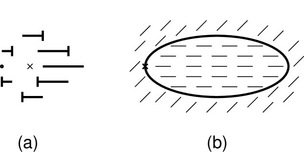
FIG. 1.: Order parameter configuration around a twist-type ring defect in a uniaxial nematic system. (a) Cross-section of the director configuration around a disclination segment running perpendicular to the page with the core passing through the point “x”. The “nail head” marks the end of the director that lies in front of the page. The director rotates by $180^{\circ}$ around the core of the disclination; the rotation axis is vertical, i.e., perpendicular to the orientation of the disclination segment. (b) The director configuration in the plane of the twist disclination loop. The director outside the disclination loop is rotated by $90^{\circ}$ with respect to the director inside the loop; the rotation axis is everywhere perpendicular to the loop plane. The cross-section shown in (a) corresponds to the configuration around the disclination segment marked by “x” in (b).

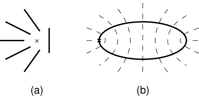
FIG. 2.: Order-parameter configuration around a wedge-type ring defect in a uniaxial nematic system. (a) Cross-section of the director configuration around a disclination segment running perpendicular to the page with the core passing through the point “x”. The director rotates by $180^{\circ}$ around the core of the disclination, with the rotation axis parallel to the orientation of the disclination segment. (b) The director configuration of the wedge disclination loop. The director is perpendicular to the loop plane everywhere inside the loop. Outside of the loop (in any plane), the director adopts the radially symmetrical configuration of a nematic hedgehog. The cross-section shown in (a) corresponds to the configuration around the disclination segment marked by “x” in (b).

D Ring defects in uniaxial nematic systems

Topologically stable disclinations lines in a uniaxial nematic cannot terminate in the bulk — they must form closed loops, or else extend to the system boundary. Depending on the details of the director configuration, the disclination loop can carry any (integral) monopole charge [34]. In this section, we discuss typical examples of disclination loops with zero and nonzero monopole charges and their contributions to the structure factor.

Consider first the case of a “twist disclination” loop, which carries zero monopole charge. The cross-section of the director configuration around a twist disclination is shown in Fig. 1a. The axis of rotation of the director is perpendicular to the direction of the disclination line. The director configuration obtained by forming a closed loop of a disclination that locally has the “twist” structure of Fig. 1a is illustrated in Fig. 1b. This director configuration is homogeneous at large distances from the loop, and consequently does not result in a power-law contribution to the structure factor for $k\ll R^{-1}$. For length scales smaller than $R$ (i.e., for $k\gg R^{-1}$), the twist disclination loop is characterized by the structure factor given in Eq. (42).

Next, consider the “wedge disclination” loop. In this configuration, the director rotates about an axis parallel to the disclination line (see Fig. 2a). The resulting director configuration (see Fig. 2b) has the structure of a radial hedgehog (see Sec. IV B) outside of the disclination loop. This results in a power-law contribution to the structure factor characterizing the nematic hedgehog in $d=3$, Eq. (35), valid for $k<R^{-1}$, where $R$ is the ring radius. On the other hand, for $k\gg R^{-1}$, we have the usual disclination-loop structure factor, Eq. (42). To summarize, the structure factor of a wedge disclination loop is given by

$$S(k)=\cases{{36\pi^{4}\over V}{1\over k^{6}},&$k\leq R^{-1}$;\cr{12\pi^{3}R\over V}{1\over k^{5}\,|\sin{\zeta}|},&$R^{-1}\ll k\ll\xi^{-1}$\,.}$$ (44)

Therefore the large-$k$ region of the structure factor measured in a system containing a wedge disclination loop of radius size $R$ is expected to exhibit a crossover between two power-law regimes with exponents $6$ and $5$ (Fig. 3). The crossover point, as defined in Fig. 3 , is predicted to occur at the value of $k_{\rm c}=3\pi\zeta/R$. Note that measuring the location $k_{\rm c}$ of the crossover allows one to obtain information about the ring-defect size $R$ from un-normalized data for $S(k)$; this should be contrasted to the use of the Porod law based on Eq. (43), where the total string length is extracted from the (rarely experimentally available) normalized structure factor.

FIG. 3.: Structure factor $S({\bf k})$ of the ring defect configuration in Fig. 2. The scattering wave-vector ${\bf k}$ is assumed to be oriented at an angle $\zeta\neq 0$ with the respect to the ring axis. The two Porod regimes, arising for length scales larger or smaller than the ring radius $R$, are shown as the dot-dashed line [$S(k)=36\pi^{4}/(Vk^{6})$] and the dotted line [$S(k)=12\pi^{3}R/(Vk^{5}|\sin{\zeta}|)$], respectively. The solid curve schematically shows the crossover between the two power-law regimes. The crossover wave-vector $k_{\rm c}$, as defined in the picture, is given by $k_{c}=3\pi R^{-1}|\sin{\zeta}|$. Thermal fluctuations can further modify the form of $S(k)$ shown in the figure, if the distance to the nearest other defect or the system boundary is large; these effects are discussed in Sec. IV E.

Even though the wedge disclination loop is a topologically admissible configuration, the (energetics-dependent) question of its occurrence in real nematic systems has recently attracted some interest. The energetic stability of the wedge loop configuration was investigated theoretically in Refs. [35] and [36]. There, it was found that provided that certain restrictions on the elastic constants in the nematic free energy are satisfied, there does indeed exist a non-zero equilibrium radius of the loop: a ring of a larger (smaller) radius will tend to shrink (expand). Depending on the values of the elastic constants, Ref. [36] predicts $R_{\rm eq}$ in the range $10\xi-10^{4}\xi$, where $\xi$ is the coherence length of the nematic order parameter (i.e., $\xi$ is of the order of $10-100\,\AA$). Note that in a nematic with a positive dielectric or diamagnetic susceptibility anisotropy, the loop can be made unstable towards expansion to a larger radius by applying an electric or magnetic field along the axis of the defect ring [37]. Wedge disclination loops with a non-zero equilibrium radius were recently observed in numerical simulations [38]. Experimental observations of such a configuration, however, are currently not available. The form of the structure factor predicted in Eq. (44), with its characteristic crossover, may be used as an experimental signature for the observation of the wedge ring configuration [54].

E Thermal fluctuations of director orientation

Up to this point, we have ignored thermal fluctuations — we have effectively assumed that the structure factor was measured at zero temperature. Nematic liquid crystalline phases, however, typically occur and are studied in the room-temperature range, and thermal effects can play an important role the scattering of light. Due to the presence of low-energy fluctuations in the orientation of the nematic director, the system exhibits enhanced turbidity throughout the whole range of temperatures where the nematic phase is stable. These transverse fluctuations of the director result in a power-law contribution to the structure factor $S(k)$, even when no defects are present in the system.

We now very briefly review the theory of scattering by thermal fluctuations in bulk uniaxial nematic liquid crystals [3, 24]. Consider a well-aligned region of the sample with the average director ${\bf u_{0}}$ parallel to the $z$-axis. The local value of the director can be written (to first order in ${\bf u_{\perp}}$) as ${\bf u}({\bf r})={\bf u_{0}}+{\bf u_{\perp}}({\bf r})$, where the transverse fluctuation ${\bf u_{\perp}}({\bf r})$, by definition, satisfies ${\bf u_{\perp}}({\bf r})\perp{\bf u_{0}}$ and we assume that $|{\bf u_{\perp}}({\bf r})|\ll 1$. The nematic structure factor, Eq. (25), then becomes [upon dropping terms proportional to $\delta(k)$]

$$S(k)={3\over 2V}{\bf u_{\perp}}({\bf k})\cdot{\bf u_{\perp}}({\bf-k})\,.$$ (45)

Note that the quantity ${\bf u_{\perp}}({\bf k})\cdot{\bf u_{\perp}}({\bf-k})$ must now be regarded as a thermal average. It’s value is readily obtained from the equipartition theorem. In the “one-constant” approximation, using ${\bf u}({\bf r})={\bf u_{0}}+{\bf u_{\perp}}({\bf r})$ in Eq. (27) results in the free energy

$$E={1\over 2}K\int{d^{3}k\over(2\pi)^{3}}k^{2}|{\bf u_{\perp}}({\bf k})|^{2}\,.$$ (46)

Furthermore, it is possible to decompose ${\bf u_{\perp}}({\bf k})$ into two orthogonal modes that decouple [3]; by equipartition, we then have $|{\bf u_{\perp}}({\bf k})|^{2}=k_{\rm B}TV$. Equation (45) thus becomes

$$S_{\rm T}(k)={3\over 2}{k_{\rm B}T\over Kk^{2}}\,.$$ (47)

Taking a typical value $K=10^{-6}$ dynes for the elastic constant and $k_{\rm B}T\simeq 0.5\cdot 10^{-13}$ erg for the thermal energy at room temperatures, one obtains the estimate

$$S_{\rm T}(k)\simeq{8{\AA}\over k^{2}}\,.$$ (48)

Note that in the light-scattering literature, the structure factor is often defined without the normalization factor $M_{\rm nem}$ in Eq. (25), and then has the dimension of volume squared, rather than of volume as in our case.

It should be stressed that Eq. (47) was derived from a free energy appropriate for small fluctuations in a well-aligned part of the nematic sample. Equation (47) can therefore be used to describe scattering from a system with a spatially varying director only provided that there are no appreciable variations in the static director orientation on the scale of $k^{-1}$.

Even in strongly inhomogeneous samples containing topological defects, thermal fluctuations will dominate the scattering intensity provided either that the defect density is sufficiently low or that $k$ is sufficiently high. To illustrate this point, we now consider light scattering from a nematic droplet of radius $R$ with normal (homeotropic) boundary conditions on the droplet surface. In the minimum-energy configuration, the droplet contains a radial hedgehog in the center. (As discussed in Sec. IV D, the radial hedgehog is, in fact, expected to take the form of a wedge disclination loop of small radius $r$; in the present paragraph, we restrict our attention to length scales exceeding $r$ and do not consider the detailed structure of the hedgehog.) Consequently, for a given scattering wave-vector $k\gg 2\pi/R$, the central region of the droplet will contribute to the structure factor according to Eq. (35), $S_{\rm def}(k)=V^{-1}36\pi^{4}k^{-6}$, where $V=4\pi R^{3}/3$. In the region $2\pi/k<r<R$, the static order-parameter configuration does not contain variations that contribute substantially to $S(k)$; however, thermal fluctuations on the scale $2\pi/k$ still exist. The contribution to $S(k)$ from these is given by Eq. (48). The resulting ratio $\gamma(k)$ of thermal and static scattering intensities, i.e. $\gamma(k)\equiv S_{\rm T}(k)/S_{\rm def}(k)=0.04(Rk)^{3}k$, where $k$ is given in inverse Å, can very in a wide range. Clearly the static contribution $S_{\rm def}(k)$ dominates when $k$ is sufficiently small (i.e. near the forward-scattered beam). Consider, on the other hand, scattering at the experimentally accessible value of $k=10^{-5}\AA^{-1}$. For a droplet of radius $R=1\,{\rm cm\/}$, we obtain $\gamma\simeq 400$; for a droplet of smaller radius $R=100\,\mu{\rm m}$, we obtain $\gamma\simeq 0.0004$. We see that either the thermal or the static contribution to the scattering intensity can completely dominate for $R$ and $k$ in the experimentally reasonable range. (For the sake of completeness we note that we have not taken into account scattering from the droplet surface in the arguments given above.)

F Porod tails in the phase-ordering kinetics of uniaxial nematics

We are now ready to discuss in detail the short-distance form of the structure factor arising during the phase-ordering process in uniaxial nematic liquid crystals, and to relate our conclusions to the experimental results reported in Refs. [7, 8].

We first briefly recall some general features of phase-ordering kinetics following a quench from a disordered to an ordered phase [39, 40]. Phase-ordering kinetics initially attracted theoretical attention due to the property of dynamical scaling of the order-parameter correlations at late times after the quench. In its simplest form, the corresponding dynamical scaling hypothesis states that all time-dependent length scales in the system have the same asymptotic time dependence (and, consequently, one can define a single “characteristic” length scale). In most systems with non-conserved order-parameter dynamics, this time-dependence is given by the power law $L(t)\propto t^{1/2}$. In systems containing topological defects, the characteristic length scale $L(t)$ can usually be extracted as the typical defect-defect separation at time $t$.

The process of phase ordering has been successfully studied experimentally in systems described by a scalar order parameter (e.g., in binary alloys—see Ref. [41]). However, analogous experiments were found to be difficult to perform in most systems with continuous symmetries (such as ferromagnets or liquid He⁴). In the recent years, a series of experiments [10, 11, 7, 8] have demonstrated that nematic liquid crystals provide a system in which phase ordering (following a quench from the isotropic to the nematic phase) is readily accessible to experimental investigation. In Refs. [7, 8], the phase-ordering process was studied by measuring the time-dependent nematic structure factor $S(k,t)$. The present section includes a discussion of the large-$k$ region of the structure factor measured in these experiments; however, we also discuss effects that may be observed under different experimental conditions.

As we saw in Secs. (IV B)–(IV D), a uniaxial nematic liquid crystalline system can contain, simultaneously, point defects (hedgehogs) and line defects (disclinations) [42]. If the average separation between hedgehogs is given by $L_{\rm hedg}$ and that between disclinations by $L_{\rm discl}$, a unit volume of the system contains $\rho_{\rm hedg}=L_{\rm hedg}^{-3}$ hedgehogs and a length $\rho_{\rm discl}=L_{\rm discl}^{-2}$ of disclinations. Now consider scattering at a wave-vector $k$ such that $k^{-1}\ll L_{\rm discl}$ and $k^{-1}\ll L_{\rm hedg}$. The total structure factor per unit volume due to hedgehogs is then given by $\rho_{\rm hedg}\,36\pi^{4}/k^{6}$ [see Eq. 35], and that due to disclinations by $\rho_{\rm discl}\,{3\pi^{3}}/k^{5}$ [see Eq. (43)]. (Here we have assumed that the disclination lines are predominantly of the twist type, as is expected from energetic considerations.) In the parts of the system that are not within distance $k^{-1}$ from the nearest disclination or hedgehog (which, by assumption, is most of the volume of the system), the static director configuration is effectively homogeneous on scales of order of $k^{-1}$. Consequently, Eq. (47) for the strength of scattering due to thermal fluctuations applies, and per unit volume, we have $S_{\rm T}(k)\simeq 8{\AA}/k^{2}$. (Notice that the length scale occurring in the expression for $S_{T}(k)$ is microscopic, as opposed to the defect separations occurring in the hedgehog and disclination contributions.) The total structure factor is therefore given by

$$S(k)=\rho_{\rm hedg}\,{36\pi^{4}\over k^{6}}+\rho_{\rm discl}\,{{3\pi^{3}}\over k^{5}}+{8{\AA}\over k^{2}}\,.$$ (49)

First consider a system in which disclinations dominate over hedgehogs. We now estimate, for a given density of disclinations $\rho_{\rm discl}$ (and $\rho_{\rm hedg}=0$), the range of scattering wave-vectors $k$ in which the the generalized Porod law behavior, $S(k)\propto k^{-5}$, can be observed. The lower limit on the range of $k$ is given by the inverse average separation of defects: $k_{\rm l}=L_{\rm discl}^{-1}=\rho_{\rm discl}^{2}$. The upper limit $k_{\rm u}$ is given by the $k$ value for which $S_{\rm T}(k)=8\,{\AA}k^{-2}$ exceeds the Porod law contribution, $S_{discl}=\rho_{\rm discl}3\pi^{3}k^{-5}$. This gives $k_{\rm u}=(3\pi^{3}/8{\AA})^{1/3}L_{d}^{-2/3}$. We see that although both $k_{\rm l}$ and $k_{\rm u}$ decrease when the separation of defects $L_{\rm discl}$ increases, the ratio $k_{\rm u}/k_{\rm l}$ increases as $(L_{\rm discl}/0.09{\AA})^{1/3}$. Analogous estimates for observing the $S(k)\propto k^{-6}$ behavior in a system dominated by hedgehogs yield $k_{\rm l}=L_{\rm hedg}^{-1}=\rho_{\rm hedg}^{3}$, $k_{\rm u}=(36\pi^{4}/8{\AA})^{1/4}L_{\rm hedg}^{-3/4}$, and $k_{\rm u}/k_{\rm l}=(L_{\rm hedg}/0.002{\AA})^{1/4}$. Consequently, the Porod form of the structure factor is predicted to extend over one to three decades in $k$ for the experimentally accessible values of defect separation of the order of $0.1\,\mu{\rm m}$ to $1\,{\rm cm}$, for either a disclination-dominated or a hedgehog-dominated system [43]. Crossover effects between $k^{-6}$ and $k^{-5}$ scaling in situations when both hedgehogs and disclinations are present may further diminish the range in which these power laws can be clearly observed. (A specific example of such behavior will be seen below.)

It should be noted that measuring the location of the crossover wave-vector $k_{\rm u}$ permits the efficient estimation of the density of defects in the system. Specifically, if one measures the location of the crossover $k_{\rm u}$ in a disclination-dominated system, the total disclination length per unit volume (expressed in units of ${\AA}^{-2}$) is given by $(2.3/k_{\rm u})^{3/2}$. In a hedgehog-dominated system, the number of hedgehogs per unit volume (expressed in units of ${\AA}^{-3}$) is given by $(4.6/k_{\rm u})^{4/3}$. Although it is also possible to estimate the defect density from the position $k_{\rm l}$ of the crossover at low wave-vectors, it should be noted that this crossover is less steep than the crossover at $k_{\rm u}$, and its precise character depends on the nature of the correlations amongst the defects.

We now relate our results to the measurements of $S(k)$ in a uniaxial nematic undergoing phase ordering in the experiments of Wong et al. [7, 8]. The range of scattering wave-vectors investigated in Refs. [7, 8] was $k=1000{\rm cm}^{-1}$–$10000{\rm cm}^{-1}$, and the typical defect separation in the system at intermediate and late times after the quench was of the order of $10\,\mu{\rm m}$ (see Fig. 1 in Ref. [7]). Direct optical observations in this and related [10, 11] phase-ordering systems indicate that disclinations dominate over hedgehogs; the exact relative proportion of their densities is, however, difficult to measure.

FIG. 4.: Theoretically predicted short-distance structure factor $S(k)$ for a 3-dimensional uniaxial nematic system undergoing phase ordering. The lower solid curve shows $S(k)$ for disclination density $\rho_{\rm discl}=10^{6}cm^{-2}$ and hedgehog density zero. The upper solid curve corresponds to disclination density $\rho_{\rm discl}=10^{6}cm^{-2}$ and hedgehog density $\rho_{\rm hedg}=10^{8}cm^{-3}$. The long-dashed, dashed, and dot-dashed lines show the contributions due to disclinations, hedgehogs, and thermal fluctuations, respectively.

In Fig. 4, we plot the structure factor $S(k)$ predicted by Eq. (49) for two situations in which the average separation between defects is of the order of $10\,\mu{\rm m}$. The lower solid curve shows $S(k)$ for $\rho_{\rm discl}=10^{6}\,{\rm cm}^{-2}$ and $\rho_{\rm hedg}=0$ (i.e., a configuration dominated by disclinations with $L_{\rm discl}=10\,\mu{\rm m}$). The upper solid curve corresponds to $\rho_{\rm discl}=10^{6}\,{\rm cm}^{-2}$ and $\rho_{\rm hedg}=10^{8}\,{\rm cm}^{-3}$ (i.e., the system contains, in addition, hedgehogs with average spacing $L_{\rm hedg}=22\,\mu{\rm m}$). We restrict the plot to the region $k>(10\,\mu{\rm m})^{-1}=10^{3}\,{\rm cm}^{-1}$, where Eq. (49) is expected to be applicable. The broken lines in Fig. 4 show the three individual contributions to $S(k)$ arising from hedgehogs, disclinations, and thermal fluctuations.

It is seen that for both $\rho_{\rm hedg}=0$ and $\rho_{\rm hedg}=10^{8}\,{\rm cm}^{-3}$, the crossover to the thermal-fluctuation-dominated regime [$S(k)\propto k^{-2}$] occurs at approximately $k=50000\,{\rm cm}^{-1}$, i.e., well beyond the range of $k$ measured in Refs. [7, 8] and at the limit of the range of $k$ accessible, in principle, with visible light. Indeed, the structure-factor data in Refs. [7, 8] do not show any sign of such a crossover. It should be noted, however, that if the scattering experiments would have been performed at a (still later) time when the average defect separation would have reached $300\,\mu{\rm m}$, the crossover value would have decreased to $k\simeq 5000\,{\rm cm}^{-1}$, and the sharp crossover to the thermal regime would have been clearly visible with the experimental setup of Refs. [7, 8] provided that the scattering probe were sufficiently sensitive.

In the case $\rho_{\rm hedg}=0$, the structure factor in Fig. 4 exhibits the Porod behavior $S(k)\propto k^{-5}$, characteristic of disclinations, over a range of 1.5 decades ($k=1000\,{\rm cm}^{-1}$ to $k=50000\,{\rm cm}^{-1}$). In the case $\rho_{\rm hedg}=10^{8}\,{\rm cm}^{-3}$, a crossover between $S(k)\propto k^{-6}$ and $S(k)\propto k^{-5}$ is spread between $k=1000\,{\rm cm}^{-1}$ and $10000\,{\rm cm}^{-1}$, and leaves only a very narrow range of $k$ for which the $S(k)\propto k^{-5}$ scaling behavior may be observed. The fact that hedgehogs result in a substantial modification of the structure factor even when $L\rho_{\rm hedg}/\rho_{\rm discl}=0.1$ is rather surprising, and is due to the large ratio, $A_{\rm hedg}/A_{\rm discl}=12\pi$, of the Porod amplitudes for hedgehogs and disclinations.

The structure-factor data reported in Refs. [7, 8] (for three-dimensional samples) were fit in these references to a power-law with exponent $6\pm 0.3$. Some of these data (specifically Fig. 7 in Ref. [8]) were later re-analyzed in Ref. [9], with the conclusion that the asymptotic slope was closer to $5$, but was approached from above , i.e., through effective exponents lying between $5$ and $6$. Our results show (see the upper solid line in Fig. 4) that such behavior is expected to arise if a sufficient number of hedgehogs is present in the system. The relative density of disclinations and hedgehogs was not examined in the experiments of Refs. [7, 8]. Other experiments investigating phase ordering in nematics, however, indicate that hedgehogs are rare compared to disclinations. (For the sake of completeness we note that it is possible to prepare nematic systems dominated by hedgehog defects: thus, in Ref. [44], a liquid crystalline system was quenched from the isotropic to the isotropic-nematic biphasic region, and a large number of hedgehogs formed upon coalescence of the nematic droplets.) Specifically, it was found in Ref. [11] that hedgehogs occurred in significant numbers only within a specific intermediate range of times after the quench, and that the ratio $L\rho_{\rm hedg}/\rho_{\rm discl}$ within this time range was of the order of $10$–$100$. The case $\rho_{\rm discl}=10^{6}\,{\rm cm}^{-2}$, $\rho_{\rm hedg}=10^{8}\,{\rm cm}^{-3}$, chosen above to obtain the upper solid curve in Fig. 4, falls within this range. Consequently, it cannot be ruled out that the observed approach to $S(k)\propto k^{-5}$ from above in Fig. 7 of Ref. [8] is due to the presence of hedgehogs, even though if the relative proportion of populations of hedgehogs and disclinations in the experiments of Refs. [7, 8] is similar to that found in the experiments of Refs. [11] (which was performed on a different nematic material), such a possibility should be considered unlikely. A more likely possibility is that a portion of the length of the disclinations in the system is of the wedge type (see Sec. IV D). Any curved configuration of a wedge disclination will lead to an order-parameter configuration in the vicinity of the disclination that resembles a part of a (radial or hyperbolic) hedgehog [45]. (The special case of a disclination loop that is wedge-like everywhere along its length was discussed in Sec. IV D; in this case, a full hedgehog configuration is obtained outside of the loop.) Although the twist configuration of a disclination line is energetically preferable to the wedge configuration for usual values of the nematic elastic constants [46], wedge-type segments of disclination loops in a system undergoing phase ordering may be generated dynamically, and lead to a $k^{-6}$ contribution to the nematic structure factor.

We complete this Section by a brief discussion of the dynamical scaling of the structure factor. Three different length scales — the disclination separation $L_{\rm discl}$, the hedgehog separation $L_{\rm hedg}$, and the microscopic length scale $8\,{\AA}$ associated with thermal fluctuations — appear in the large-$k$ form of the nematic structure factor, Eq. (49). Is this inconsistent with the property of dynamical scaling of the structure factor, according to which there exists a (time-dependent) length scale $L(t)$ such that $k^{3}S(k)$ depends only on the dimensionless scaling variable $y\equiv kL(t)$? Let us choose the disclination separation $L_{\rm discl}$ as the characteristic length $L(t)$. From Eq. (49), we then have

$$k^{3}S(y)={3\pi^{3}}{1\over y^{2}}+{36\pi^{4}\over y^{3}}\left[{L_{\rm discl}(t)\over L_{\rm hedg}(t)}\right]^{3}+y{8{\AA}\over L_{\rm discl}(t)}\,.$$ (50)

Clearly, $k^{3}S(k)$ does not in general satisfy the scaling form $f(kL_{\rm discl}(t))$. At asymptotically late times, however, $L_{\rm discl}\gg 8{\AA}$ and, consequently, the term in Eq. (50) associated with thermal fluctuations becomes negligible. Experimental evidence [11] indicates that at late times after the quench, the hedgehog separation $L_{\rm hedg}(t)$ grows faster than the disclination separation $L_{\rm discl}(t)$. Consequently, the second term in Eq. (50) (associated with hedgehogs) also becomes negligible, asymptotically. Our analysis is therefore consistent with the dynamical scaling of the structure factor at asymptotically late times. As we saw earlier in this Section, however, the scattering contributions from thermal fluctuations and from nematic hedgehogs can lead to significant transient effects under typical experimental conditions.

V Biaxial nematic systems

Thus far, our discussion of defects in nematics has concentrated on the case of uniaxial systems. It is straightforward to generalize this discussion to the case of biaxial [3] systems. As there are no topologically stable point defects in a three-dimensional biaxial nematic [47], we need only consider line defects. Biaxial nematics admits four topologically distinct classes of line defects [47], which are disclination lines distinguished by the angles of rotation of the uniaxial director ${\bf u}$ and the biaxial director ${\bf b}$ [defined in Eq. (22)] around the defect core. In the $C_{x}$ class of disclinations ${\bf u}$ rotates by $\pm 180^{\circ}$ and ${\bf b}$ does not rotate; in $C_{y}$ disclinations ${\bf u}$ does not rotate and ${\bf b}$ rotates by $\pm 180^{\circ}$; in $C_{z}$ disclinations both ${\bf u}$ and ${\bf b}$ rotate by $\pm 180^{\circ}$; finally, in $\overline{C}_{0}$ disclinations either ${\bf u}$ or ${\bf b}$ (or both) rotate by $360^{\circ}$. These four distinct disclination types were observed experimentally in a thermotropic nematic polymer [21], and their properties where found to be in agreement with the predictions of the topological classification scheme.

In the minimum-energy configuration [with free energy given by Eq. (27] for the $C_{x}$, $C_{y}$, and $C_{z}$ defects, the $180^{\circ}$ rotations of the ${\bf u}$ and ${\bf b}$ director are uniform [48]. The configuration of a $C_{x}$ disclination is correspondingly given (up to a global rotation) by Eq. (22) with

$${\bf u}({\bf x}) = \big{(}\cos{1\over{2}}\phi({\bf x}),\sin{1\over{2}}\phi({\bf x}),0\big{)},$$ (52)

$${\bf b}({\bf x}) = \big{(}0,0,1\big{)},$$ (53)

$${\bf v}({\bf x}) = \big{(}\cos\big{(}{1\over{2}}\phi({\bf x})+{\pi\over{4}}\big{)},\sin\big{(}{1\over{2}}\phi({\bf x})+{\pi\over{4}}\big{)},0\big{)},$$ (54)

where $\phi({\bf x})$ is the polar angle in the plane perpendicular to the disclination line. The correlation function (23) for this configuration can be expressed (up to an additive constant) as the correlation function (38) for the uniaxial nematic disclination, multiplied by the biaxiality-strength–dependent factor $R(3S_{1}+S_{2})^{2}/4$, where $R\equiv 3S_{1}^{2}/(3S_{1}^{2}+S_{2}^{2})$ is the ratio of the uniaxial ($S_{2}=0$) and biaxial ($S_{2}\neq 0$) normalization factors $M_{\rm nem}$. The corresponding factors for the case of the $C_{y}$ and $C_{z}$ disclinations are likewise readily evaluated. By using the result (43) for the uniaxial disclination, we obtain the structure factors of the biaxial disclinations $C_{x}$, $C_{y}$ and $C_{z}$:

$$S(k)_{\rm C_{x}} = {9\pi^{2}\over 8}{L_{x}\over V}{S_{1}^{2}(3S_{1}+S_{2})^{2}\over 3S_{1}^{2}+S_{2}^{2}}{1\over k^{5}}\,,$$ (56)

$$S(k)_{\rm C_{y}} = {9\pi^{2}\over 2}{L_{y}\over V}{S_{1}^{2}S_{2}^{2}\over 3S_{1}^{2}+S_{2}^{2}}{1\over k^{5}}\,,$$ (57)

$$S(k)_{\rm C_{z}} = {9\pi^{2}\over 8}{L_{z}\over V}{S_{1}^{2}(3S_{1}-S_{2})^{2}\over 3S_{1}^{2}+S_{2}^{2}}{1\over k^{5}}\,.$$ (58)

It should be noted that in the case $3S_{1}=S_{2}$, the amplitude in the Porod law for the $C_{z}$ defect is zero, whereas the amplitudes for the $C_{x}$ and $C_{y}$ defects are non-zero and equal to each other [see Eqs. (56)–(58)]. This reflects the fact that for $3S_{1}=S_{2}$, the order parameter given by Eq. (22) describes a uniaxial discotic phase [49] with uniaxial axis ${\bf v}={\bf u}\times{\bf b}$. Correspondingly, the $C_{z}$ configuration in this case does not represent a defect (as ${\bf v}$ does not rotate), whereas the $C_{x}$ and $C_{y}$ configurations are equivalent.

It remains to consider the ${\overline{C}_{0}}$ disclination. For the case $S_{1}>S_{2}$ (i.e., needle-like ordering [49]), the minimum-energy configuration of type ${\overline{C}_{0}}$ is given by Eq. (22) with

$${\bf u}({\bf x}) = \big{(}0,0,1\big{)},$$ (60)

$${\bf b}({\bf x}) = \big{(}\cos\phi({\bf x}),\sin\phi({\bf x}),0\big{)},$$ (61)

$${\bf v}({\bf x}) = \big{(}\cos\big{(}\phi({\bf x})+\pi/4\big{)},\sin\big{(}\phi({\bf x})+\pi/4\big{)},0\big{)},$$ (62)

where $\phi({\bf x})$ is the polar angle in the plane perpendicular to the disclination line. The correlation function (23) for the point defect in the planar cross-section through this disclination can then be expressed as $R(2S_{2}/3S_{1})^{2}$, By using Eq. (20) one obtains the structure factor per unit length of the ${\overline{C}_{0}}$ disclination:

$$S(k)_{\rm\overline{C}_{0}}=12\pi^{2}{L_{0}\over V}{S_{2}^{2}\over 3S_{1}^{2}+S_{2}^{2}}{1\over k^{5}}\,.$$ (63)

For the case $S_{1}<S_{2}$ (i.e., discotic ordering [49]) the ${\bf v}$ director (and not the ${\bf u}$ director, in contrast with the needle-like case) corresponds to the eigenvalue of the order-parameter tensor $Q_{\alpha\beta}$ largest in absolute value, and the lowest energy configuration that can be taken by the ${\overline{C}_{0}}$ disclination has directors given by

$${\bf u}({\bf x}) = \big{(}\cos\phi({\bf x}),\sin\phi({\bf x}),0\big{)},$$ (65)

$${\bf b}({\bf x}) = \big{(}\cos\big{(}\phi({\bf x})+{\pi\over{4}}\big{)},\sin\big{(}\phi({\bf x})+{\pi\over{4}}\big{)},0\big{)},$$ (66)

$${\bf v}({\bf x}) = \big{(}0,0,1\big{)}\,.$$ (67)

The corresponding structure factor is

$$S(k)_{\rm\overline{C}_{0}}={8\over 3}{L_{0}\over V}\pi^{2}{(3S_{1}^{2}-S_{2})^{2}\over 3S_{1}^{2}+S_{2}^{2}}{1\over k^{5}}\,.$$ (68)

In general, the large-$k$ structure factor of a biaxial nematic system is given by the sum of the expressions (56-57) and (63) or (68).

Finally, we note that in a biaxial nematic film (i.e., a system having two spatial dimensions, but the full $3\times 3$ tensorial nematic parameter), $C_{x}$, $C_{y}$, $C_{z}$ and ${\overline{C}_{0}}$ are point-like defects (the dynamics of which was studied in [22]). The Porod-law amplitudes for these defects are obtained from the amplitudes in the results (56)–(58), (63) and (68) by dividing by $\pi$ [see Eq. (20)], and the corresponding Porod-law exponents take the value 4 instead of 5.

VI Corrections to Porod’s law

In this section we briefly discuss several effects—inter-defect interactions, inequality among the three elastic constants in the nematic free energy, curvature of linear defects, and the presence of the defect core—that were not fully taken into account during our calculations in the previous sections and may, under certain circumstances, lead to modifications of our results.

An interesting question, already alluded to in Sec. II, is whether the order-parameter configuration in the vicinity of the defect core is or is not affected by the interactions with the other defects present in the system. [In order to avoid confusion with the core region, where the order parameter magnitude is reduced, we shall refer to the region close to, but outside, the core, as the “central” region of the defect.] It is important to distinguish between static and dynamic effects. In the case of the $O(2)$ vector model with the standard gradient free energy, given by Eq. (6), the minimum-energy configuration of a collection of defects with fixed locations is obtained simply by taking the superposition of the angles characterizing the order parameter ${\bf m}$ around isolated defects; their central regions are therefore unaffected. A deformation does occur, however, once the defects are allowed to move [50]; for sufficiently slow defect velocities, this effect may be neglected.

The situation is different in the $O(3)$ vector-model case. Here, Ostlund [28] showed that in the minimum-energy configuration of a monopole-antimonopole pair separated by a fixed distance, the gradient free energy is concentrated along a string connecting the two point defects. We are not aware of any investigation of how this result might be modified in a dynamical situation. Ostlund’s result does suggest, however, that the order-parameter configuration of monopoles and antimonopoles in a phase-ordering $O(3)$ vector system in $d=3$ may substantially differ from the radially symmetric configuration assumed during the calculation of the corresponding Porod law in Sec. III A of the present Paper.

Consider, then, an arbitrary point defect in the $O(N)$ vector model in $d=N$ dimensions. We denote the corresponding order-parameter configuration by ${\bf\Phi}({\bf r})$, where the radius-vector ${\bf r}$ originates at the core of the defect. As already indicated in Sec. II, the value $\xi=2d$ of the Porod exponent for point defects is suggested by simple dimensional analysis, independently of the exact form of ${\bf\Phi}({\bf r})$. This argument can be made more precise if we consider configurations in which ${\bf\Phi}({\bf r})$ depends only on the direction ${\bf{\hat{r}}}$, and not the magnitude $r$, of the radius-vector ${\bf r}$. We may write ${\bf\Phi}({\bf k})\equiv\int d^{d}r\,e^{i{\bf k}\cdot{\bf r}}{\bf\Phi}({\bf r})=\int d^{d}r\,e^{ik{\bf{\hat{k}}}\cdot{\bf r}}{\bf\Phi}({\bf r})$; by assumption, ${\bf\Phi}(k^{-1}{\bf r})={\bf\Phi}({\bf r})$, which, combined with the substitution ${\bf r}=k^{-1}{\bf y}$, yields ${\bf\Phi}({\bf k})=k^{-d}\int d^{d}y\,e^{i{\bf{\hat{k}}}\cdot{\bf y}}{\bf\Phi}({\bf y})\equiv k^{-d}\,\,{\bf\Phi}({\bf{\hat{k}}})$. Consequently, the structure factor Eq. (4) is of the form $S({\bf k})=A({\bf{\hat{k}}})k^{-2d}$, where the Porod amplitude $A({\bf{\hat{k}}})\equiv M_{\rm O(N)}^{-1}{\bf\Phi}({\bf{\hat{k}}})\cdot{\bf\Phi}(-{\bf{\hat{k}}})$ now depends on the orientation of ${\bf k}$. The Porod exponent $\xi=2d$, expressing how $S({\bf k})$ depends on the magnitude of ${\bf k}$, is, however, unchanged compared to the radially symmetric case. As for the value of $A({\bf{\hat{k}}})$, we may make the following argument using the identity relating the standard form of the gradient free energy $E$ to the structure factor $S({\bf k})$:

$$E\equiv{\kappa\over 2}\int d^{d}x\,\nabla_{i}\Phi_{j}({\bf x})\nabla_{i}\Phi_{j}({\bf x})={\kappa\over 2}\int\,d^{d}k\,k^{2}S({\bf k})={\kappa\over 2}\big{\langle}A({\bf{\hat{k}}})\big{\rangle}_{\rm ang}\int^{\xi^{-1}}_{D^{-1}}\,dk\,k^{2-2d}\,.$$ (69)

Here $\big{\langle}A({\bf{\hat{k}}})\big{\rangle}_{\rm ang}$ denotes the angular average of $A({\bf{\hat{k}}})$ over all orientations ${\bf{\hat{k}}}$, $\kappa$ is a positive elasticity constant, $\xi$ is the core size of the defect and $D$ is the large-distance cutoff necessary in the calculation of the free energy. Equation (69) implies that $\big{\langle}A({\bf{\hat{k}}})\big{\rangle}_{\rm ang}$ reaches its minimum for the order-parameter configuration ${\bf\Phi}({\bf{\hat{r}}})$ that minimizes the free energy $E$ [51]. In the case of the $O(N)$ monopole with charge $+1$, the configuration minimizing $E$ is precisely the radial configuration used by us in Sec. III A, and we conclude that our result Eq. (14) provides a lower bound for the value of the Porod amplitude in a macroscopically isotropic system [52].

Note, however, that the property of $\big{\langle}A({\bf{\hat{k}}})\big{\rangle}_{\rm ang}$ formulated above applies equally well for defects that do not possess radial symmetry in the minimum-energy configuration, such as monopoles with higher-integer charges in the $O(N)$ vector model, or strength-$1/2$ disclinations in nematic liquid crystals [in the latter case, $E$ in Eq. (69) is replaced by the Frank free energy in the one-constant approximation, Eq. (27)]. We thus reach the conclusion that in nematics for which the three elastic constants (see Sec. IV A) are not equal to each other and consequently, the configuration of the nematic director around a disclination differs from the configuration minimizing Eq. (27), the angle-averaged structure factor in a phase-ordering system will have Porod amplitudes larger than those derived by us in Secs. IV B–IV F, even when the central regions of the defects are not deformed by inter-defect interactions.

While deriving the results for linear defects [$O(3)$ vortex lines in Sec. III B and nematic disclinations in Secs. IV C and IV D], we assumed that the curvature $1/R$ of the defect lines was negligible (i.e. $Rk\gg 1$). In general, we can expect corrections to the basic Porod law $k^{-5}$ that are suppressed by factors of $Rk$, thus resulting in contributions to $S(k)$ decaying as higher power laws ($k^{-\eta}$ with $\eta>5$). The case of curved wedge-type disclinations (discussed near the end of Sec. IV C), for which $\eta=6$, serves as an example.

Similarly, we can expect higher-power terms to arise from the presence of the core region of the defects. As the crossing of the boundary between the core region and the outside region of a defect is associated with a change in the magnitude of the order parameter, we may obtain an upper-bound estimate of the corresponding contribution $S_{\rm core}(k)$ to the structure factor by regarding the core boundary as a domain wall in a scalar system, leading (in a 3-dimensional system) to $S_{\rm core}(k)\simeq ak^{-4}$, where $a$ is the domain wall area. For a monopole $a\simeq\xi^{2}$, where $\xi$ is the core size, and the ratio of $S_{\rm core}(k)$ to the standard monopole contribution $k^{-6}$ is of the order of $(\xi k)^{-2}$. For a string defect of length $L$, we have $a\simeq\xi L$, and the ratio of $S_{\rm core}(k)$ to $Lk^{-5}$ is of the order of $\xi k$. For typical core sizes $\xi$ of the order of $10\AA$ and for scattering wave-vector values $k\leq 10^{-4}\AA$ accessible with visible light, we have $\xi k\geq 1000$, and the contributions to $S(k)$ from the defect core are expected to be negligible for both monopoles and strings.

VII Conclusions

In this Paper we have presented a detailed discussion of the influence of topological defects on the large-wavevector behavior of the structure factor $S({\bf k})$ in nematic liquid crystals. The presence of topological defects leads to power-law contributions to $S({\bf k})$ of the Porod form $\rho Ak^{-\xi}$, where $\rho$ is the number density of a given type of defect, $A$ is a dimensionless amplitude, and $\xi$ is an integer-valued exponent. We have computed the values of the Porod exponents and amplitudes for the various types of topological defects present in uniaxial and biaxial nematics, and have discussed the competition between contributions to $S({\bf k})$ due to defects and to thermal fluctuations.

Our main results are summarized in Tables I (for nematic films) and II (for bulk nematic systems). To obtain the short-distance structure factor of a nematic system containing topological defects, the expressions given in Tables I or II should be multiplied by the number densities of the corresponding defects and then added. Here, the defect number density is defined as the number of point defects, resp. the total length of line defects, per unit area (in a two-dimensional system) or unit volume (in a three-dimensional system). In addition, the total structure factor contains a power-law contribution due to transverse thermal fluctuations of the nematic director, this contribution being given (in a bulk system) approximately by $8{\AA}/k^{2}$. The resulting form of the structure factor $S(k)$ is valid for $k$ ranging from the inverse typical separation of defects to the inverse defect-core size.

TABLE I.: Power-law contributions to the structure factor arising from topological defects in systems with spatial dimension $d=2$. Results are given per unit defect density (see Sec. VII). For biaxial nematics, $S_{1}$ and $S_{2}$ denote the uniaxial and biaxial amplitudes of the nematic order parameter, and $C_{x}$, $C_{y}$ and $C_{z}$ denote the three topologically distinct $180^{\circ}$ defect types (see Sec. V).

	Uniaxial	Biaxial	O(2) vector	O(3) vector
	nematic	nematic	model	model
$180^{\circ}$ disclination point	$3\pi^{2}k^{-4}$	$C_{x}:\,\,\,\,\,{9\pi^{2}\over 8}{S_{1}^{2}(3S_{1}+S_{2})^{2}\over 3S_{1}^{2}+S_{2}^{2}}k^{-4}$	does not exist	topologically
		$C_{y}:\,\,\,\,\,{9\pi^{2}\over 2}{S_{1}^{2}S_{2}^{2}\over 3S_{1}^{2}+S_{2}^{2}}k^{-4}$		unstable
		$C_{z}:\,\,\,\,\,{9\pi^{2}\over 8}{S_{1}^{2}(3S_{1}-S_{2})^{2}\over 3S_{1}^{2}+S_{2}^{2}}k^{-4}$
$360^{\circ}$ disclination point	topologically	$(S_{1}>S_{2}):\,\,\,\,\,{S_{2}^{2}\over 3S_{1}^{2}+S_{2}^{2}}k^{-4}$	$4\pi^{2}k^{-4}$	topologically
	unstable	$(S_{1}<S_{2}):\,\,\,\,\,{8\over 3}\pi^{2}{(3S_{1}^{2}-S_{2})^{2}\over 3S_{1}^{2}+S_{2}^{2}}k^{-4}$		unstable

TABLE II.: Power-law contributions to the structure factor arising from topological defects in systems with spatial dimension $d=3$. The results given in the first three rows are given per unit defect density (see Sec. VII). The results in the fourth (fifth) row correspond to a single twist (wedge) circular disclination loop of radius $R$ in a system of volume $V$; $\zeta$ denotes the angle between the scattering wave-vector ${\bf k}$ and the loop axis. For biaxial nematics, $S_{1}$ and $S_{2}$ denote the uniaxial and biaxial amplitudes of the nematic order parameter, and $C_{x}$, $C_{y}$ and $C_{z}$ denote the three topologically distinct $180^{\circ}$ defect types (see Sec. V).

	Uniaxial	Biaxial	O(2) vector	O(3) vector
	nematic	nematic	model	model
Hedgehog defect	$36\pi^{4}k^{-6}$	does not exist	does not exist	$12\pi^{3}k^{-6}$
		$C_{x}:\,\,\,\,\,{9\pi^{3}\over 8}{S_{1}^{2}(3S_{1}+S_{2})^{2}\over 3S_{1}^{2}+S_{2}^{2}}k^{-5}$
$180^{\circ}$ disclination line	${3\pi^{3}}k^{-5}$	$C_{y}:\,\,\,\,\,{9\pi^{3}\over 2}{S_{1}^{2}S_{2}^{2}\over 3S_{1}^{2}+S_{2}^{2}}k^{-5}$	does not exist	does not exist
(orientational average)		$C_{z}:\,\,\,\,\,{9\pi^{3}\over 8}{S_{1}^{2}(3S_{1}-S_{2})^{2}\over 3S_{1}^{2}+S_{2}^{2}}k^{-5}$
$360^{\circ}$ disclination line	topologically	$(S_{1}>S_{2}):\,\,\,\,\,\pi{S_{2}^{2}\over 3S_{1}^{2}+S_{2}^{2}}k^{-5}$	$4\pi^{3}k^{-5}$	topologically
(orientational average)	unstable	$(S_{1}<S_{2}):\,\,\,\,\,{8\over 3}\pi^{3}{(3S_{1}^{2}-S_{2})^{2}\over 3S_{1}^{2}+S_{2}^{2}}k^{-5}$		unstable
		$C_{x}:\,\,\,\,\,{9\pi^{3}\over 2}{S_{1}^{2}(3S_{1}+S_{2})^{2}\over 3S_{1}^{2}+S_{2}^{2}}{R\over V}k^{-5}/|\sin{\zeta}|$
Twist disclin. loop	$12\pi^{3}{R\over V}k^{-5}/|\sin{\zeta}|$	$C_{y}:\,\,\,\,\,{18\pi^{3}}{S_{1}^{2}S_{2}^{2}\over 3S_{1}^{2}+S_{2}^{2}}{R\over V}k^{-5}/|\sin{\zeta}|$	$16\pi^{3}{R\over V}k^{-5}/|\sin{\zeta}|$	does not exist
		$C_{z}:\,\,\,\,\,{9\pi^{3}\over 2}{S_{1}^{2}(3S_{1}-S_{2})^{2}\over 3S_{1}^{2}+S_{2}^{2}}{R\over V}k^{-5}/|\sin{\zeta}|$
Wedge disclin. loop	$\cases{{36\pi^{4}\over V}k^{-6},&$k\leq R^{-1}$\cr 12\pi^{3}{R\over V}k^{-5}/|\sin{\zeta}|,&$k>R^{-1}$}$	does not exist	does not exist	does not exist

To avoid confusion, we remind the reader that our results were calculated for a structure factor $S({\bf k})$ defined so that the real-space correlation function $C({\bf r})$ is normalized to unity at $r=0$ (and, consequently, our structure factor has the dimension of volume). Thus, our results differ from the un-normalized structure factor (with dimension of volume squared) by the normalization factor $M_{\rm norm}=(V/2)(3S_{1}^{2}+S_{2}^{2})$ (where $V$ is the system volume or area, $S_{1}$ is the (uniaxial) order-parameter magnitude, and $S_{2}$ is the strength of biaxial ordering). Recall, in addition, that the scattered-light intensity is directly proportional to the structure factor $S({\bf k})$ only in the case of unpolarized light scattering. Finally, recall (Sec. VI) that the values of the Porod amplitudes (but not those of the Porod exponents) in the general case of unequal elastic constants in the Frank free energy (26) are expected to differ from the values (derived in the one-constant approximation) listed in Tables I and II .

For comparison, we also show in Tables I and II the results for the corresponding defects (when they exist) in $O(2)$ and $O(3)$ symmetric vector-model systems. In these systems, the normalization factor $M_{\rm norm}$ is given by $Vs^{2}$, where $s$ is the order-parameter magnitude. Identical results for some of the $O(N)$ defect configurations were previously obtained in Ref. [20].

We conclude this Paper by highlighting some features of our results. As discussed in Sec. II, the value of the Porod exponent $\xi$ can be correctly anticipated purely on dimensional grounds. It should be noted, however, that the value of the dimensionless Porod amplitude $A$ often differs considerably from unity. For example, in the case of the nematic hedgehog defect, we obtained $A=36\pi^{4}\simeq 3500$. In addition, the Porod amplitude depends significantly on the order parameter in question (and not just on the spatial and defect dimensionalities). For example, the Porod amplitude for the nematic hedgehog exceeds the amplitude for the $O(3)$ monopole in $d=3$ by a factor of $3\pi$.

In Secs. IV E and IV F, we analyzed in detail the conditions under which the Porod tail of the structure factor is not overshadowed by the power-law contribution from transverse thermal fluctuations of the nematic director. [Similar considerations apply to any system possessing continuous symmetry of the order parameter.] We concluded that for experimentally accessible defect densities in a nematic phase-ordering experiment, the Porod tail should be observable over a range of 1 to 3 decades in $k$; the range of observability is limited by defect interactions at small $k$ and by thermal fluctuations at large $k$. In the experiments reported in Refs. [7, 8], the measured structure factor did exhibit a Porod tail over at least 1 decade in $k$, but the crossover at high $k$ to the fluctuation-dominated regime was not observed. This was found to be consistent with our theoretical predictions under the conditions of these experiments.

The crossover from $S(k)\propto k^{-5}$ (in a system where disclinations dominate over hedgehogs) to $S(k)\propto k^{-2}$ (the thermal-fluctuation-dominated regime) was predicted in Sec. IV F to occur approximately at the scattering wave-vector value $k_{\rm u}=(3\pi^{3}/8{\AA})^{1/3}L_{\rm discl}^{-2/3}$, where $L_{\rm discl}$ is the total disclination length per unit volume of the system. As this crossover is very sharp, and is not affected by defect interactions, measuring $k_{\rm u}$ can give a precise estimate of the total disclination length. We are not aware of any use of this method in the experimental literature to date. The proportionality of the Porod tail to the defect density has been used previously [7, 8] to extract the power law characterizing the decay of disclination length; extracting the absolute defect density in this way, however, would require the knowledge of the (rarely experimentally available) normalized structure factor. The location of the crossover $k_{\rm u}$, on the other hand, can be extracted from the unnormalized structure factor.

In Sec. IV D, we contrasted the contributions to the structure factor arising from twist-type and wedge-type disclination loops. The wedge-type loop of radius $R$ gives a $k^{-6}$ contribution at $k<R^{-1}$ in addition to the usual $k^{-5}$ disclination contribution at $k>R^{-1}$, as it has the structure of a nematic hedgehog at large distances from the loop. Likewise, any curved disclination segment of the wedge type gives rise to a $k^{-6}$ contribution. In Sec. IV F, we attempted to connect these findings to the observation that the structure factor in phase-ordering uniaxial nematics approaches the $k^{-5}$ power law at high $k$ through effective exponents larger than 5 (and close to 6) at intermediate $k$. Such a behavior of the structure factor had been found to occur in experiments [7, 8] as well as in numerical simulations [29], but not in approximate analytical theories [9]. We concluded that it was, in principle, possible, but nevertheless unlikely, that the “approach from above” to the exponent $\chi=5$ observed in the experiments was due to $k^{-6}$ contributions from hedgehog defects. It remains a challenge for future work to determine whether this behavior of the structure factor is caused by hedgehog defects, curved wedge-type disclination segments, or correlations that fall beyond the range of the Porod regime.

- [1] Electronic address: martinz@lubensky.physics.upenn.edu
- [2] Electronic address: goldbart@uiuc.edu
- [3] P.-G. de Gennes and J. Prost, The Physics of Liquid Crystals (Clarendon, Oxford, 1993).
- [4] P. Chatelain, Acta Cristallogr. 1, 315 (1948).
- [5] P.-G. de Gennes, C. R. Acad. Sci. (Paris) 266, 15 (1968).
- [6] D. Langevin and M. Bouchiat, J. Phys. (Paris) Colloq. 36 (Suppl. C1), 197 (1975).
- [7] A. P. Y. Wong, P. Wiltzius and B. Yurke, Phys. Rev. Lett. 69, 3583 (1992).
- [8] A. P. Y. Wong, P. Wiltzius, R. G. Larson and B. Yurke, Phys. Rev. E 47, 2683 (1993).
- [9] A. J. Bray, S. Puri, R. E. Blundell and A. M. Somoza, Phys. Rev. E 47, 2261 (1993).
- [10] I. Chuang, R. Durrer, N. Turok and B. Yurke, Science 251, 1336 (1991).
- [11] I. Chuang, B. Yurke, A. N. Pargelis and N. Turok, Phys. Rev. E 47, 3343 (1993).
- [12] H. Orihara, T. Nagaya, and Y. Ishibashi, in Formation, Dynamics and Statistics of Patterns, edited by K. Kawasaki and S. Suzuki (World Scientific, 1993).
- [13] M. J. Bowick, L. Chandar, and E. A. Schiff, Science 263, 943 (1994).
- [14] P. T. Mather, D. S. Pearson, R. G. Larson, Liquid Crystals 20, 527 (1996); Liquid Crystals 20, 539 (1996).
- [15] S. Kai, W. Zimmermann, and M. Andoh, Mod. Phys. Lett. B 4, 767 (1990).
- [16] D. J. Graziano and M. R. Mackley, Mol. Cryst. Liq. Cryst. 106, 73 (1984).
- [17] M. Kléman, L. Liébert, and L. Strzelecki, Polymer 24, 295 (1983).
- [18] R. G. Larson, Constitutive Equations for Polymer Melts and Solutions (Butterworths, New York, 1988).
- [19] L. M. Blinov and V. G. Chigrinov, Electrooptic Effects in Liquid Crystal Materials (Springer-Verlag, New York, 1994).
- [20] A. J. Bray and K. Humayun, Phys. Rev. E 47, 9 (1993).
- [21] T. De’Nève, M. Kléman and P. Navard, J. Phys. II (France) 2, 187 (1992).
- [22] M. Zapotocky, P. M. Goldbart and N. Goldenfeld, Phys. Rev. E 51, 1216 (1995).
- [23] See, e.g., D. C. Champeney, Fourier transforms and their physical applications, (Academic Press, London, 1973).
- [24] We do not discuss thermal fluctuations at the lower criticial dimension , where the situation is more complicated.
- [25] See, e.g., N. Goldenfeld, Lectures on Phase Transitions and the Renormalization Group (Addison-Wesley, Reading, 1992).
- [26] P. Debye, H. R. Anderson and H. Brumberger, J. Appl. Phys. 28, 679 (1957).
- [27] G. Porod, in Small-Angle X-Ray Scattering, edited by O. Glatter and O. Kratky (Academic, New York, 1982).
- [28] S. Ostlund, Phys. Rev. B 24, 485 (1981).
- [29] R. E. Blundell and A. J. Bray, Phys. Rev. E 49, 4925 (1994).
- [30] This method was already used in Ref. [31] to obtain the Porod exponent for defects in the two-dimensional symmetric vector model.
- [31] M. Mondello and N. Goldenfeld, Phys. Rev. A 45, 657 (1992).
- [32] If is perpendicular to the plane of the loop, then from Eq. (17) we see that the total structure factor is , where for finite has the meaning of a function with a sharp peak around having a half-width of the order of . Consequently, we obtain a zero contribution to for .
- [33] N. D. Mermin, Rev. Mod. Phys. 51, 591 (1979).
- [34] H. Nakanishi, K. Hayashi and H. Mori, Commun. Math. Phys. 117, 203 (1988).
- [35] H. Mori and H. Nakanishi, J. Phys. Soc. Jpn. 57, 1281 (1988).
- [36] O. D. Lavrentovich, T. Ishikawa and E. M. Terentjev, Mol. Cryst. Liq. Cryst. A 304, 463 (1997).
- [37] V. G. Bondar, O. D. Lavrentovich, and V. M. Pergamenschik, Zh. Exp. Teor. Fiz. 101, 111 (1991) [Sov. Phys. JETP 74, 60 (1992)].
- [38] H. Toyoki, J. Phys. Soc. Jpn. 63, 4446 (1994).
- [39] J. D. Gunton, M. San Miguel and P. S. Sahni, in Phase Transitions and Critical Phenomena, Vol. 8, C. Domb and J. L. Lebowitz, Eds. (Academic Press, New York, 1983).
- [40] A. J. Bray, Adv. Phys. 43, 357 (1994).
- [41] B. D. Gaulin, S. Spooner and Y. Morii, Phys. Rev. Lett. 59, 668 (1987).
- [42] In addition to the two types of singular defects (hedgehogs and disclinations), non-singular topologically stable objects— topological textures [33]—can occur in uniaxial nematics. A single-texture configuration, however, does not result in a power-law contribution to the structure factor. Furthermore, these objects were not found to occur naturally in the phase-ordering experiments reported in Ref. [10]. We shall not be concerned with topological textures in the present Paper.
- [43] We note, however, that if the sample is placed in an external magnetic or electric field, large- thermal fluctuations are suppressed in the regions of the sample where the director is aligned along the field [3]. This can lead to an increase of the upper limit of the Porod regime.
- [44] A. N. Pargelis, J. Mendez, M. Srinivasarao, and B. Yurke, Phys. Rev. E 53, R25 (1996).
- [45] M. Zapotocky and T. C. Lubensky, unpublished.
- [46] S. Chandrasekhar and G. S. Ranganath, Adv. Phys. 35, 507 (1986).
- [47] See, e.g., Ref. [33].
- [48] Ch. Kobdaj and S. Thomas, Nucl. Phys. B 438, 607 (1995).
- [49] See Ref. [3], or the discussion in Sec. II of Ref. [22].
- [50] L. M. Pismen and J. D. Rodriguez, Phys. Rev. A 42, 2471 (1990).
- [51] It is worth noting that Eq. (69) can be used as an indirect means of evaluating the orientation-averaged Porod amplitude in the cases where the energy of the defect configuration is known.
- [52] Indeed, it was found in analytical investigations (A. D. Rutenberg, unpublished) of the Porod law corresponding to a point defect in the model in that the Porod amplitude increased (and the Porod exponent remained unchanged) when the symmetrical defect configuration was deformed.
- [53] In general, the director rotates in any way such that two antipodal points in the nematic order-parameter space are connected upon encircling the disclination core, and the disclination is not necessarily of either the wedge type or the twist type.
- [54] Note that the Porod-law regime with exponent is expected to be absent from the structure factor contribution arising from wedge-type satellite defect rings that have been predicted to occur under certain conditions around macroscopic particles suspended in a nematic liquid crystal [see, e.g., E. M. Terentjev, Phys. Rev. E 51, 1330 (1995)]. Here, the effect of the wedge-type ring defect is to compensate for the radial boundary condition on the director at the surface of the particle, thus permitting a homogeneous director configuration at large distances from the particle (without the need for other particles or defects).