Quantifying spatially heterogeneous dynamics in computer simulations of glass-forming liquids

Abstract

We examine the phenomenon of dynamical heterogeneity in computer simulations of an equilibrium, glass-forming liquid. We describe several approaches to quantify the spatial correlation of single-particle motion, and show that spatial correlations of particle displacements become increasingly long-range as the temperature decreases toward the mode coupling critical temperature.

Proceedings of the 1998 Pisa Workshop on Supercooled Liquids and Glassy Materials.

1 Introduction

Liquids cooled toward their glass transition exhibit remarkable dynamical behavior [1]. The initial slowing down of many liquids at temperatures well above their glass transition temperature $T_{g}$ can be described to great extent by the mode coupling theory [2, 3, 4], which predicts diverging relaxation times at a dynamical critical temperature $T_{c}$ despite the absence of a diverging or even growing static correlation length [5]. At the same time, experiments in the temperature range $T_{g}<T<T_{c}$, and simulations in the range $T>T_{c}$, have shown that it is possible to select subsets of particles in the liquid (or monomers in the case of polymers) that move differently from the bulk on time scales less than the structural relaxation time [6, 7, 8, 9]. The question then arises as to whether glass-forming liquids exhibit spatially heterogeneous dynamics, and if so, is there a growing length scale associated with this dynamical heterogeneity?

We have employed three complementary computational approaches to address this question:

1. Subset approach. In this approach [10, 11, 12], we monitor the displacement of each particle in a time window $\Delta t$, rank the displacements from largest to smallest, and examine spatial correlations within subsets of particles exhibiting either extremely large or extremely small displacements. In this way, we have demonstrated that particles of similar mobility form clusters that grow with decreasing temperature $T$. Moreover, particles exhibiting the largest displacements within a time window in the late-$\beta$/early-$\alpha$ relaxation regime (“mobile” particles) form low-dimensional clusters that grow and percolate at the mode coupling transition temperature $T_{c}$.

2. Displacement-displacement correlation function approach. In this approach [13, 14, 15], we monitor the displacement of each particle in a time window $\Delta t$ as above, and calculate a bulk, equilibrium correlation function that measures the correlations between the local fluctuations in the particle displacements. Because this approach does not rely on defining subsets via arbitrary thresholds or cutoffs, it may prove more amenable to future analytical treatment.

3. First passage time approach. In this approach [16], we monitor the first passage time $\tau$ for each particle to move a distance $\epsilon$, and then for a given $\epsilon$, examine spatial correlations between the different $\tau$ values either by grouping particles into subsets of similar $\tau$, or by calculating a $\tau$-$\tau$ correlation function using all the particles. This approach shows that particles with similar first passage times to travel any $\epsilon$ are spatially correlated. It also allows us to identify particular values of $\epsilon$ for which the first passage times are most correlated, and thereby extract detailed information on, e.g., the cage size.

In this paper, we present results from the first two approaches outlined above, and show that as an equilibrium Lennard-Jones liquid approaches $T_{c}$, correlations between local fluctuations in particle displacements develop, grow, become increasingly long-ranged, and appear to diverge at $T_{c}$. Similar results for a simulated polymer blend are presented elsewhere [17].

2 Theory

Consider a liquid confined to a volume $V$, consisting of $N$ identical particles, each with no internal degrees of freedom. Let the position of each particle $i$ be denoted ${\mbox{\boldmath$r$\unboldmath}}_{i}$. The motion of a particle $i$ may be described by its displacement $\mu_{i}(t,\Delta t)\equiv|{\mbox{\boldmath$r$\unboldmath}}_{i}(t+\Delta t)-{\mbox{\boldmath$r$\unboldmath}}_{i}(t)|$ over some interval of time $\Delta t$, starting from a reference time $t$. The question of whether particle motions in a liquid are correlated can be addressed by modifying the usual definition of the density-density correlation function $G({\mbox{\boldmath$r$\unboldmath}})$ (which measures spatial correlations of fluctuations in local density away from the average value [18, 19]) so that the contribution of each particle $i$ to $G({\mbox{\boldmath$r$\unboldmath}})$ is weighted by $\mu_{i}$. Thus, we define a “displacement-displacement” correlation function [13, 14, 15, 20],

$$G_{u}({\mbox{\boldmath$r$\unboldmath}},\Delta t)=\int d{\mbox{\boldmath$r$\unboldmath}^{\prime}}\Bigl{\langle}\bigl{[}u({\mbox{\boldmath$r$\unboldmath}^{\prime}}+{\mbox{\boldmath$r$\unboldmath}},t,\Delta t)-\langle u\rangle\bigr{]}\,\bigl{[}u({\mbox{\boldmath$r$\unboldmath}^{\prime}},t,\Delta t)-\langle u\rangle\bigr{]}\Bigl{\rangle},$$ (1)

where

$$u({\mbox{\boldmath$r$\unboldmath}},t,\Delta t)=\sum_{i=1}^{N}\mu_{i}(t,\Delta t)\,\delta\bigl{(}{\mbox{\boldmath$r$\unboldmath}}-{\mbox{\boldmath$r$\unboldmath}}_{i}(t)\bigr{)}.$$ (2)

and where $\langle\cdots\rangle$ denotes an ensemble average. $G_{u}({\mbox{\boldmath$r$\unboldmath}},\Delta t)$ measures the correlations of fluctuations of local displacements away from their average value. Since we are considering an equilibrium liquid, and because $G_{u}$ is defined as an ensemble average, $G_{u}$ does not depend on the choice of the reference time $t$. For the same reasons, $\langle u\rangle\equiv\langle u({\mbox{\boldmath$r$\unboldmath}},t,\Delta t)\rangle$ only depends on $\Delta t$ for a homogeneous, equilibrium liquid.

$G_{u}({\mbox{\boldmath$r$\unboldmath}},\Delta t)$ can be separated into self and distinct parts, so that we can identify a spatial correlation function $g_{u}({\mbox{\boldmath$r$\unboldmath}},\Delta t)$ analogous to the static pair correlation function $g({\mbox{\boldmath$r$\unboldmath}})$ conventionally used to characterize the structure of a liquid [18]:

$$G_{u}({\mbox{\boldmath$r$\unboldmath}},\Delta t)={\bigl{\langle}N\bigr{\rangle}}{\overline{\mu^{2}}}\,\delta({\mbox{\boldmath$r$\unboldmath}})+\langle u\rangle\langle U\rangle\,[g_{u}({\mbox{\boldmath$r$\unboldmath}},\Delta t)-1],$$ (3)

where

$$g_{u}({\mbox{\boldmath$r$\unboldmath}},\Delta t)={{1}\over{\langle u\rangle\langle U\rangle}}\Biggl{\langle}\sum_{i=1}^{N}\sum_{{\scriptstyle j=1}\atop{\scriptstyle j\neq i}}^{N}\mu_{i}(t,\Delta t)\,\mu_{j}(t,\Delta t)\,\delta\bigl{(}{\mbox{\boldmath$r$\unboldmath}}+{\mbox{\boldmath$r$\unboldmath}}_{j}(t)-{\mbox{\boldmath$r$\unboldmath}}_{i}(t)\bigr{)}\Biggl{\rangle}.$$ (4)

Here we have defined the “total displacement” $U$ as $U(t,\Delta t)=\int d{\mbox{\boldmath$r$\unboldmath}}\,u({\mbox{\boldmath$r$\unboldmath}},t,\Delta t)$, and its ensemble average $\langle U\rangle\equiv\langle U(t,\Delta t)\rangle$. We have also defined ${\bar{\mu}}\equiv\bigl{\langle}\frac{1}{N}\sum_{i=1}^{N}\mu_{i}(t,\Delta t)\bigr{\rangle}$, and ${\overline{\mu^{2}}}\equiv\bigl{\langle}\frac{1}{N}\sum_{i=1}^{N}\mu_{i}^{2}(t,\Delta t)\bigr{\rangle}$. In a constant-$N$ ensemble, $\langle u\rangle$ and $\langle U\rangle$ are readily evaluated as $\bigl{\langle}u\bigr{\rangle}=\rho\,{\bar{\mu}}$ and $\bigl{\langle}U\bigr{\rangle}=N\,{\bar{\mu}}$. Note that $g_{u}(r,\Delta t)$ is different from the distinct part of the time-dependent van Hove correlation function $g(r,t)$, because it correlates information between pairs of particles using information about the position of each particle at two different times. Thus $g_{u}(r,\Delta t)$ is in some sense a four-point correlation function, whereas $g(r,t)$ is a two-point correlation function.

A “structure factor” for the particle displacements can be defined as

$$S_{u}({\mbox{\boldmath$q$\unboldmath}},\Delta t)\equiv\Biggl{\langle}\frac{1}{N{\overline{\mu^{2}}}}\sum_{i=1}^{N}\sum_{j=1}^{N}\mu_{i}(t,\Delta t)\mu_{j}(t,\Delta t)\exp\left[-i{\mbox{\boldmath$q$\unboldmath}}\cdot({\mbox{\boldmath$r$\unboldmath}}_{i}(t)-{\mbox{\boldmath$r$\unboldmath}}_{j}(t))\right]\Biggr{\rangle}.$$ (5)

The fluctuations of $U$ are related to the volume integral of $G_{u}({\mbox{\boldmath$r$\unboldmath}},\Delta t)$:

$$\Bigl{\langle}\bigl{[}U-\bigl{\langle}U\bigr{\rangle}\bigr{]}^{2}\Bigr{\rangle}=\int d{\mbox{\boldmath$r$\unboldmath}}\,G_{u}({\mbox{\boldmath$r$\unboldmath}},\Delta t)\equiv\bigl{\langle}U\bigr{\rangle}\bigl{\langle}u\bigr{\rangle}kT\kappa_{u},$$ (6)

where $k$ is Boltzmann’s constant. Recall that the volume integral of the density-density correlation function $G({\mbox{\boldmath$r$\unboldmath}})$ is proportional to the isothermal compressibility $\kappa$, which diverges at a conventional critical point because $G({\mbox{\boldmath$r$\unboldmath}})$ becomes long-ranged. Likewise, the fluctuations in $U$ will provide information regarding the range of $G_{u}({\mbox{\boldmath$r$\unboldmath}},\Delta t)$. Thus, in analogy with conventional critical phenomena, we have defined an isothermal “susceptibility” $\kappa_{u}$.

For a fixed choice of $\Delta t$, note that if the displacement were always the same for every particle, then $g_{u}({\mbox{\boldmath$r$\unboldmath}},\Delta t)$ and $g({\mbox{\boldmath$r$\unboldmath}})$ would be identical for all $r$ (and $S_{u}({\mbox{\boldmath$q$\unboldmath}},\Delta t)$ and $S({\mbox{\boldmath$q$\unboldmath}})$ would be identical for all $q$). Hence, it is deviations of $g_{u}({\mbox{\boldmath$r$\unboldmath}},\Delta t)$ ($S_{u}({\mbox{\boldmath$q$\unboldmath}},\Delta t)$) from $g({\mbox{\boldmath$r$\unboldmath}})$ ($S({\mbox{\boldmath$q$\unboldmath}})$) that will inform us of correlations of fluctuations of local displacements away from the average value, that are in excess of those that would be expected based on a knowledge of $g({\mbox{\boldmath$r$\unboldmath}})$ or $S({\mbox{\boldmath$q$\unboldmath}})$ alone.

3 Simulation Details

We have measured the spatial correlations in particle displacements using data obtained [10, 11, 12] from a molecular dynamics simulation of a model Lennard-Jones glass-former. The system is a three-dimensional binary mixture (80:20) of 8000 particles interacting via Lennard-Jones interaction parameters [21]. We analyze data from seven $(\rho,P,T)$ state points that lie on a line in the $P,T$ plane, approaching the mode-coupling dynamical critical temperature $T_{c}\approx 0.435$ at a pressure $P_{c}\approx 3.03$ and density $\rho_{c}\approx 1.2$ [22] (all values are quoted in reduced units [21]). The highest and lowest temperature state points simulated are $(\rho=1.09,P=0.50,T=0.550)$ and $(\rho=1.19,P=2.68,T=0.451)$, respectively. Following equilibration at each state point, the particle displacements are monitored in the NVE ensemble for up to $1.2\times 10^{4}$ Lennard-Jones time units (25.4 ns in argon units) for the coldest $T$. Complete simulation details may be found in [12].

For all seven state points, a “plateau” exists in both the mean square displacement and the intermediate scattering function $F_{s}({\mbox{\boldmath$q$\unboldmath}},t)$ as a function of $t$ [12]. The plateau separates an early time ballistic regime from a late time diffusive regime, and indicates “caging” of the particles typical of low $T$, high density liquids. The same model liquid, simulated along a different path toward the same mode coupling critical point, was found to be well described by the ideal mode coupling theory [22]. For the present (larger) simulation, the $\alpha$-relaxation time $\tau_{\alpha}$ that describes the long-time decay of $F_{s}({\mbox{\boldmath$q$\unboldmath}},t)$ at the value of $q$ corresponding to the first peak in the static structure factor $S({\mbox{\boldmath$q$\unboldmath}})$ increases by 2.4 orders of magnitude, and follows a power law $\tau_{\alpha}\sim(T-T_{c})^{-\gamma}$, with $T_{c}\simeq 0.435$ and $\gamma\simeq 2.8$. The diffusion coefficient $D$ is found to behave as $D\sim(T-0.435)^{2.13}$. The simulated liquid states analyzed here therefore exhibit the complex bulk relaxation behavior characteristic of a supercooled liquid approaching its glass transition.

4 Results

Throughout the following subsection, all quantities are calculated using all 8000 particles in the system. Results do not change substantially if the minority particles are not included in the analysis. In the cluster analysis in Subsection 4.2, only the majority particles are included in the analysis. However, our results do not change quantitatively when the minority particles are included. Recall that in the mode coupling analysis of this model liquid by Kob and Andersen, the same mode coupling transition temperature was found for the majority particles as for the minority particles [22].

4.1 Displacement-displacement correlation function

$S_{u}(q,\Delta t)$ is shown for different $T$ in Fig. 1, calculated for a value of $\Delta t$ chosen on the order of $\tau_{\alpha}$ for each $T$. For intermediate and large $q$, $S_{u}(q,\Delta t)$ coincides with the static structure factor $S({\mbox{\boldmath$q$\unboldmath}})\equiv\Bigl{\langle}\frac{1}{N}\sum_{i=1}^{N}\sum_{j=1}^{N}\exp\left[{-i{\mbox{\boldmath$q$\unboldmath}}\cdot({\mbox{\boldmath$r$\unboldmath}}_{i}-{\mbox{\boldmath$r$\unboldmath}}_{j})}\right]\Bigr{\rangle}$ (see inset). However, for $q\rightarrow 0$ a peak in $S_{u}(q,\Delta t)$ develops and grows with decreasing $T$, suggesting the presence of increasing long range correlations in $G_{u}({\mbox{\boldmath$r$\unboldmath}},\Delta t)$. No such growing peak at $q=0$ appears in the static structure factor $S(q)$ (cf. inset), indicating the absence of long range correlations in the particle positions.

Figure 1: Displacement “structure factor” $S_{u}(q,\Delta t)$ for different $T$. The $q=0$ values are obtained from $S_{u}(q=0,\Delta t)=({\overline{\mu}}^{2}/{\overline{\mu^{2}}})\,\rho kT\kappa_{u}$. INSET: Static structure factor $S(q)$ for four different $T$.

Indeed, a comparison of $g_{u}(r,\Delta t)$ and $g(r)$ shows that at every $T$ simulated, the particle displacements are more correlated than their positions. At the lowest $T$, this excess correlation persists for values of $r$ up to 6 interparticle distances [15].

In Fig.1 $\Delta t$ is chosen on the timescale of the $\alpha$-relaxation time. The significance of the time interval $\Delta t$ can be seen by examining the “susceptibility” $\kappa_{u}(\Delta t)$. Here we have calculated $\kappa_{u}(\Delta t)$ directly from the fluctuations in the total displacement $U$. Fig. 2 demonstrates four important points: (i) As $\Delta t\to 0$, $\kappa_{u}\to 0$. Note that in the limit $\Delta t\to 0$, $\mu_{i}(t,\Delta t)/\Delta t$ is equal to the magnitude of the instantaneous velocity. Thus correlations cannot be observed by looking at a “snapshot” of the system, that is, by measuring correlations in the instantaneous velocity [23]. (ii) Initially, as $\Delta t$ increases, $\kappa_{u}$ increases. Thus the spatial correlation of particle displacements develops over time. (iii) There is a time window $\Delta t^{*}$ during which $\kappa_{u}$ is maximum. Both the maximum value of $\kappa_{u}$ and corresponding time window $\Delta t^{*}$ increase with decreasing $T$. (iv) As $\Delta t\to\infty$, $\kappa_{u}$ decreases. Thus in the diffusive regime, where the particles act like Brownian particles, there are no correlations in the particle motions.

Figure 2: $\kappa_{u}(\Delta t)$ as a function of $\Delta t$ for different temperatures.

Fig. 3 shows that the time $\Delta t^{*}$ at which the fluctuations in the particle displacements are a maximum follows a power law with T: an excellent fit to the form $\Delta t^{*}\sim(T-T_{c})^{-\gamma}$ is obtained when $T_{c}=0.435\pm 0.005$, and yields $\gamma=2.3\pm 0.3$, where the highest value of $\gamma$ is obtained with the lower bound on $T_{c}$. Our estimated value for $\gamma$ differs from that describing the divergence at $T_{c}$ of the structural relaxation time $\tau_{\alpha}$ ($\gamma\simeq 2.8$), but (within our numerical uncertainty) cannot be distinguished from the exponent governing the apparent vanishing of the diffusion coefficient $D$ ($\gamma\simeq 2.1\pm 0.1$).

Figure 3: Time when the fluctuations in the particle displacements are largest, plotted vs. temperature. The solid curve is a fit to $\Delta t^{*}\sim(T-0.435)^{-2.3}$. INSET: $\Delta t^{*}$ vs. $\tau_{\alpha}$, plotted log-log. The solid line has slope $0.81$, and represents the best fit curve through the data. The dashed line has slope $1.0$, and is not nearly as good a fit. That $\Delta t^{*}$ does not scale linearly with $\tau_{\alpha}$ is further supported by the fact that an exponent less than $2.6$ describing the apparent divergence of $\tau_{\alpha}$ with $T-T_{c}$ can be excluded.

In Fig 4 we show the $T$-dependence of $\kappa_{u}(\Delta t^{*})$. We find that $\kappa_{u}(\Delta t^{*})$ grows monotonically with decreasing $T$, indicating that the range of the correlation measured by $g_{u}(r,\Delta t^{*})$ is growing with decreasing $T$. The data can be fitted extremely well with a power law $\kappa_{u}(\Delta t^{*})\sim(T-T_{c})^{-\gamma}$ with $T_{c}=0.435$, and yields $\gamma=0.84$. (As shown in the figure, a larger (closer to Curie-Weiss-type) exponent can be obtained by fitting the data with a power law that diverges at a slightly lower value of $T_{c}$.) Thus the previously determined mode coupling critical temperature coincides, within our numerical error, with the temperature where $G_{u}(r,\Delta t)$ becomes long ranged.

Figure 4: “Susceptibility” $\kappa_{u}(\Delta t^{*})$ versus temperature. The solid and dashed curves are power law fits to the data, as indicated in the figure.

The displacement-displacement correlation function measures the tendency for particles of similar mobility to be spatially correlated (cf. Fig. 5).

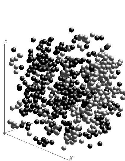
Figure 5: Particles exhibiting the 5% largest (light) and 5% smallest (dark) displacements in $\Delta t^{*}$ starting from an arbitrary time origin, at $T=0.451$. The clustering of particles of similar mobility is evident in the figure.

To extract a correlation length from the data, we have attempted to fit $S_{u}(q,\Delta t^{*})$ using an Orstein-Zernike form, $S_{u}(q,\Delta t^{*})\propto 1/(1+\xi^{2}q^{2})$. This form assumes that $G_{u}({\mbox{\boldmath$r$\unboldmath}},\Delta t^{*})$ is asymptotically proportional to $e^{-r/\xi}/r$, where $\xi$ is the correlation length [19]. We find that this form fits well at the highest $T$ but fails to fit the data on approaching $T_{c}$. The data can instead be fitted at all $T$ using the more general form $S_{u}(q,\Delta t^{*})\propto 1/(1+(\xi q)^{\eta})$. The best fit gives $\eta=1.99$ and 3.54 for our highest and lowest $T$, respectively. However, because $\eta$ depends on $T$, $\xi$ does not show a definite trend with temperature, giving values of roughly three particle diameters. Larger simulations may be required to accurately determine the correct functional form for $S_{u}$ at small $q$. Nevertheless, the data show unambiguously that as $T\to T_{c}$, spatial correlations between the displacements of particles arise and grow and become long-ranged at $T_{c}$. To obtain further evidence for a growing dynamical length scale, we turn now to the subset method described in the Introduction [24].

4.2 Cluster analysis of mobile particles

Examination of the distribution of particle displacements (the self part of the usual time-dependent van Hove correlation function [18]) immediately shows the problems inherent in defining subsets of particles of extremely low mobility. Over the time range coincident with the plateau in the mean square displacement, this function exhibits a narrow peak containing most of the particles, and a long tail to large distances containing a small percentage of the particles. The non-Gaussian parameter $\alpha_{2}(t)$ has been used to identify a time when this tail is most pronounced [10]. At that time, approximately 95% of the particles are contained in the peak, and about 5% are contained in the tail, regardless of temperature. Because of this tail, the most mobile particles in the liquid “distinguish” themselves from the bulk, while it is more difficult to define a threshold with which to identify particles exhibiting extremely small displacements (“immobile” particles).

By examining the maximum displacement achieved by a particle in a time window $\Delta t$, a somewhat better definition of immobility can be achieved. It was shown in Ref. [12] that particles exhibiting the smallest displacement defined in this way are spatially correlated, and form relatively compact clusters. Using this definition of maximum displacement, which for the most mobile particles gives the same results as the simple definition of displacement used above, we find that highly mobile particles also cluster. These clusters are very ramified, and are composed of smaller “strings” of particles that follow one another (cf. Fig. 6).

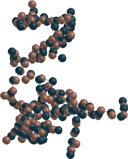
Figure 6: A large cluster of mobile particles found at $T=0.451$, at two different times. Pink denotes the particles at $t=0$ and blue denotes the particles at time $\Delta t$ later, where $\Delta t$ is slightly less than $\Delta t^{*}$. The small black lines connect the same particle at the two times. Thus between $t=0$ and $\Delta t$, each particle shown has moved almost one interparticle distance. This cluster can be decomposed into a number of elementary “cooperatively rearranging strings”, defined as minimal groups of particles that follow one another [11, 25].

In this subsection, we are interested in the growth of clusters of highly mobile particles with decreasing temperature. To this end, we have constructed clusters of nearest neighbor particles whose maximum displacement in a time window $\Delta t\sim\Delta t^{*}$ falls within the top 3%, 5% and 7% of all displacements [12]. The distribution of clusters of size $n$ constructed using the top 5% of the particles is shown in the inset of Fig. 7 for four different $T$. Also shown in Fig. 7 is the $T$-dependence of the mean cluster size $S=\sum n^{2}P(n)/\sum nP(n)$ for each subset [26]. We find that for each subset $S\sim(T-T_{p})^{-\gamma}$ with $T_{p}=0.440,0.431$, and $0.428$, all close to $T_{c}$. (Note that as the number of particles contained in the subset increases, $T_{p}$ decreases.) For the subset containing 5%, the data fall on a straight line when plotted log-log against $T-T_{c}$. Thus, we conclude that $T_{c}$ appears to coincide with a percolation transition of the most mobile particles in the liquid.

Figure 7: Mean cluster size $S$ plotted versus $T$, for subsets containing 3% (circles), 5% (squares), and 7% (diamonds) of the most mobile particles at $T=0.451$. The lines are power law fits $S\sim(T-T_{p})^{-\gamma}$. Best fit parameters are $T_{p}=0.440,0.431$ and $0.428$, respectively, and $\gamma=0.397,0.687$, and $0.741$, respectively. INSET: Distribution of the size $n$ of clusters of mobile particles for four different $T$.

The presence of clusters of mobile particles whose size grows with decreasing temperature contributes to the growing range of the displacement-displacement correlation function. Thus we can use the mean cluster size to give a rough estimate of the length scale on which particle motions are correlated. In our coldest simulation, the mean cluster size is approximately $10$ particles. Since the clusters have a fractal dimension of approximately 1.75 [12], that implies a mean radius of gyration larger than 3 particle diameters. The largest cluster observed at $T=0.451$ contains over 100 particles, and thus has a radius of gyration that exceeds the size of our simulation box at that $T$.

It is important to note that while the mean size of clusters of mobile particles appears to diverge at $T_{c}$, the smaller, cooperatively rearranging “strings” that make up these clusters also grow with decreasing $T$, but are still finite at $T_{c}$ [11]. In the temperature regime studied here, the distribution of string lengths is exponential, and the mean string length appears to diverge at a temperature substantially lower than $T_{c}$. Thus while the mode coupling transition may coincide with a percolation transition of clusters of highly mobile particles, our data is compatible with the idea of Adam and Gibbs that the ideal glass transition at $T_{o}<T_{c}$ is associated with the growth and possible divergence of the minimum size of a cooperatively rearranging region (“strings” in the present simulation). This idea will be further explored elsewhere [25].

5 Discussion

In this paper, we have defined a bulk correlation function that quantifies the spatial correlation of single-particle displacements in a liquid, and we have examined spatial correlations within subsets of highly mobile particles. While the first approach has the advantage of allowing a direct calculation of spatial correlations in local particle motions without having to define arbitrary subsets, the second approach has the advantage of permitting a geometrical analysis of clusters of highly mobile and highly immobile particles. Using both approaches, we have shown in computer simulations of an equilibrium Lennard-Jones liquid that the displacements of particles are spatially correlated [27] over a range and time scale that both grow with decreasing $T$ as the mode coupling transition is approached. While mode coupling theory currently makes no predictions concerning a growing dynamical correlation length, calculation of the vector analog of the displacement-displacement correlation function should be tractable within the mode-coupling framework. Finally, the displacement-displacement correlation function has allowed us to identify a fluctuating dynamical variable U whose fluctuations become longer ranged and appear to diverge at $T_{c}$. In this regard, $U$ is behaving much like a static order parameter on approaching a second-order static critical point, suggesting the possibility that we can obtain insights into the nature of glass-forming liquids using an extension to dynamically-defined quantities of the framework of ordinary critical phenomena.

6 References

References

- [1] M. D. Ediger, C. A. Angell, and S. R. Nagel 1996 J. Phys. Chem. 100 13200.
- [2] W. Götze and L. Sjogren 1996 Chem. Phys. 212 47; W. Götze and L. Sjogren 1995 Transport Theory Stat. Phys. 24 801.
- [3] H.Z. Cummins, these proceedings.
- [4] See the special issue of Transport Theory Stat. Phys. 24 devoted to experimental and computational tests of MCT.
- [5] See, e.g., A. van Blaaderen and P. Wiltzius 1995 Science 270 1177, and R. Leheny, et al 1996 J. Chem. Phys. 105 7783.
- [6] K. Schmidt-Rohr and H.W. Spiess 1991 Phys. Rev. Lett. 66 3020.
- [7] R. Böhmer, R.V. Chamberlain, G. Diezemann, B. Geil, A. Heuer, G. Hinze, S.C. Kuebler, R. Richert, B. Schiener, H. Sillescu, H.W. Spiess, U. Tracht and M. Wilhelm 1998 J. Non-Cryst. Solids 235-237 1, and the many references therein.
- [8] See, e.g., M.T. Cicerone and M.D. Ediger 1995 J. Chem. Phys. 103 5684.
- [9] For a review, see H. Sillescu J. Non-Cryst. Solids in press.
- [10] W. Kob, C. Donati, S.J. Plimpton, P.H. Poole and S.C. Glotzer 1997 Phys. Rev. Lett. 79 2827.
- [11] C. Donati, J.F. Douglas, W. Kob, S.J. Plimpton, P.H. Poole and S.C. Glotzer 1998 Phys. Rev. Lett. 80 2338.
- [12] C. Donati, S.C. Glotzer, P.H. Poole, W. Kob, and S.J. Plimpton, cond-mat/9810060.
- [13] S.C. Glotzer, C. Donati and P.H. Poole 1998 in Computer Simulation Studies in Condensed-Matter Physics XI, edited by D.P. Landau, et al. (Springer-Verlag, Berlin) (in press).
- [14] P.H. Poole, C. Donati and S.C. Glotzer Physica A in press.
- [15] C. Donati, P.H. Poole and S.C. Glotzer, cond-mat/9811145.
- [16] P. Allegrini, J.F. Douglas and S.C. Glotzer, in preparation; P. Allegrini and S.C. Glotzer, in preparation.
- [17] C. Bennemann, C. Donati, J. Baschnagel, and S.C. Glotzer, preprint.
- [18] J. P. Hansen and I.R. McDonald 1986 Theory of Simple Liquids (Academic Press, London).
- [19] H.E. Stanley 1971 Introduction to Phase Transitions and Critical Phenomena (Oxford University Press, New York).
- [20] A related correlation function has been calculated for the Ising spin glass in S.C. Glotzer, N. Jan, T. Lookman, A.B. MacIsaac, and P.H. Poole 1998 Phys. Rev. E 57 7350.
- [21] The Lennard-Jones interaction parameters and are given by: , , , , , . Lengths are defined in units of , temperature in units of , and time in units of . Both types of particles are taken to have the same mass.
- [22] W. Kob and H. C. Andersen 1994 Phys. Rev. Lett. 73 1376; W. Kob and H. C. Andersen 1995 Phys. Rev. E 51 4626; 1995 Phys. Rev. E 52, 4134.
- [23] Correlations of particle motions on short time scales has been studied in 2-d simulations by Y. Hiwatari and T. Muranaka 1998 J. Non-crystalline Solids 235-237, 19, and references therein.
- [24] Indirect evidence for a growing length from studies of glassforming liquids or polymers in confined geometries is reported in, e.g. M. Arndt, et al., Phys. Rev. Lett. 79, 2077 (1997); B. Jerome and J. Commandeur, Nature 387, 589 (1997); and P. Ray and K. Binder, Europhysics Lett. 27, 53 (1994). A “hydrodynamic” correlation length was calculated for a LJ liquid by R. Mountain in Supercooled Liquids: Advances and Novel Applications, ACS Symposium Series 676, 122 (1987).
- [25] P. Allegrini, C. Donati, J.F. Douglas and S.C. Glotzer, in preparation.
- [26] D. Stauffer 1995 Introduction to Percolation Theory (Taylor & Francis Ltd, London).
- [27] Other recent computational investigations of spatially heterogeneous dynamics include Y. Yamamoto and A. Onuki 1998 Phys. Rev. E 58 3515; D. Perera and P. Harrowell 1998 J. Non-cryst. Sol. 235-237 314; B. Doliwa and A. Heuer 1998 Phys. Rev. Lett. 80 4915; Ref. [23].