Mean-field theory of temperature cycling experiments in spin-glasses

Leticia F. Cugliandolo
Laboratoire de Physique Théorique de l’École Normale Supérieure de Paris
24, rue Lhomond, 75231, Paris, France

and

Laboratoire de Physique Théorique et Hautes Énergies, Jussieu,
4, Place Jussieu, 75005, Paris, France

leticia@physique.ens.fr

Jorge Kurchan
Laboratoire de Physique de l’École Normale Supérieure de Lyon
46, Allée d’Italie, Lyon, France

Jorge.Kurchan@enslapp.ens-lyon.fr

Abstract

We study analytically the effect of temperature cyclings in mean-field spin-glasses. In accordance with real experiments, we obtain a strong reinitialization of the dynamics on decreasing the temperature combined with memory effects when the original high temperature is restored. The same calculation applied to mean-field models of structural glasses shows no such reinitialization, again in accordance with experiments. In this context, we derive some relations between experimentally accessible quantities and propose new experimental protocols. Finally, we briefly discuss the effect of field cyclings during isothermal aging.

LPT-ENS/9842; LPTHE/9853.

Glasses are characterized by having extremely slow relaxations and by the strong dependence of their behaviour upon the (“waiting”) time elapsed since their preparation. The latter property is usually called physical aging.

A means to study the dynamics in the glassy phase in more detail consists in following the evolution of the sample under a complicated temperature history. The protocols that have been more commonly used include temperature cyclings within the low temperature phase.

The results for different types of glasses are quite different. [1, 2, 3, 4, 5, 6, 7, 8, 9] Spin-glasses show the puzzling phenomenon of reinitialization of aging following a decrease in temperature, combined with the recall of the situation attained before the negative jump when the original high temperature is restored.[2, 4] Remarkably, when similar protocols were applied to structural glasses, e.g. in dielectric constant measurements of glycerol by Leheny and Nagel,[9] no substantial reinitialization was observed.[10]

This difference in the effect of temperature changes on spin and structural glasses is a fact that any generic theory of glasses is expected to explain.

Different groups interpreted the behaviour of spin-glasses under temperature cyclings during aging as evidence for both the droplet[5, 7] and the hierarchical[6] pictures of the dynamics (the former with some extra refinement [7] with respect to the original versions of the eighties[11]).

The hierarchical dynamic picture[12, 6] is a heuristic way to think about the results from positive and negative cyclings inspired in the organization of equilibrium states in the Parisi solution of mean-field spin-glasses, such as the Sherrington-Kirkpatrick model. It is assumed that spin-glasses have a large number of metastable states that are organized in a hierarchical fashion just like the equilibrium states. It is then proposed that the system is composed of (independent) subsystems whose dynamics is given by the wandering in such a landscape. An average over subsystems has to be invoked in order to obtain smooth results as observed in experiments.

A concrete realisation of a hierarchical dynamic system can be made with the trap models.[13, 14, 15] These models have been solved analytically in isothermal conditions.[15] Though a full analytic description of their dynamics in the presence of temperature cyclings is not available yet, a careful discussion of their effects yields very encouraging results.[15]

Surprisingly enough, the main features of the cycling experiments have never been derived analytically from microscopic models, while the numerical evidence[24, 25, 26, 27] is inconclusive. In this paper we shall show analytically how these effects arise in mean-field models of spin glasses, and why they are absent in mean field models of structural glasses. One of the questions that will receive a clear answer is why the effects should be hardly observable at very short times, such as are inevitably involved in simulations.

We shall consider in detail the particular class of temperature cycling experiments in which the thermoremanent magnetization (TRM) is measured. Similar conclusions have been extracted from the out of phase susceptibility ($\chi^{\prime\prime}$) data at fixed frequency.[2, 29]

There is however a slight difference between TRM and ac $\chi^{\prime\prime}$ measurements. In the former the TRM after the cycling is recorded and, since measurements are directly performed in the time domain, one has access to very large time scales after $t_{w}$. In the latter case the $\chi^{\prime\prime}$ is measured during and after the cycling This allows us, for example, to clearly see the large reinitialization of the dynamics provoked by the negative jump.[2] The price to pay is that in ac measurements the frequencies are necessarily small compared to to the inverse of the measuring time. One then has access to relatively small time-differences.

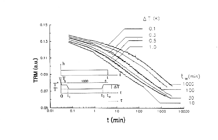
FIG. 1.: The TRM curves after a long negative cycle sketched in the inset. The temperature at which the relaxation is measured is $T=12K=0.72\,T_{g}$. The bold lines are reference curves corresponding to waiting at a constant temperature of $12K$ during $t_{w}=10,\,30,\,100,\,1000$ min. The thin lines are obtained after a temperature cycling of $1000$ min and temperature jumps $\Delta T=0.1,\,0.3,\,0.5,\,1\,K$. The data is courtesy of E. Vincent, see Ref. [2].

In the TRM experiments of Refregier et al.[2] the system is quenched to a subcritical temperature under a small field that is used as a probe, for which the linearity in the response is checked within the same experiment.

In the negative temperature cycling experiment (see the inset of Fig. 1), the system is quenched at $t=0$ to a temperature $T^{+}$. At a time $t_{1}$ the temperature is dropped to $T^{-}$ and at a later time $t_{2}$ the temperature $T^{+}$ is restored. The fraction of time spent at $T^{-}$ is rather large.

The resulting state of the sample after the temperature cycling is investigated by cutting off the field at a time $t_{w}$ soon after $t_{2}$ and by recording the subsequent decay of the TRM. The results for different $\Delta T$ are shown in Fig. 1: The TRM curves for each $\Delta T$ can be superposed to the TRM curves obtained at constant $T^{+}$ but with an effective waiting time $t_{1}+t_{w}-t_{2}\leq t_{w}^{\sc eff}(\Delta T,t_{1},t_{2},t_{w})\leq t_{w}$. Note that the first inequality implies that the system remembers the evolution performed at the higher temperature $T^{+}$ while the time spent at the lower temperature $T^{-}$ is partially (or even totally) erased.

Once the negative cycle is over, its main effect is to slow down the aging process. This result is very intuitive and will hold for almost any system with slow dynamics activated by thermal noise.

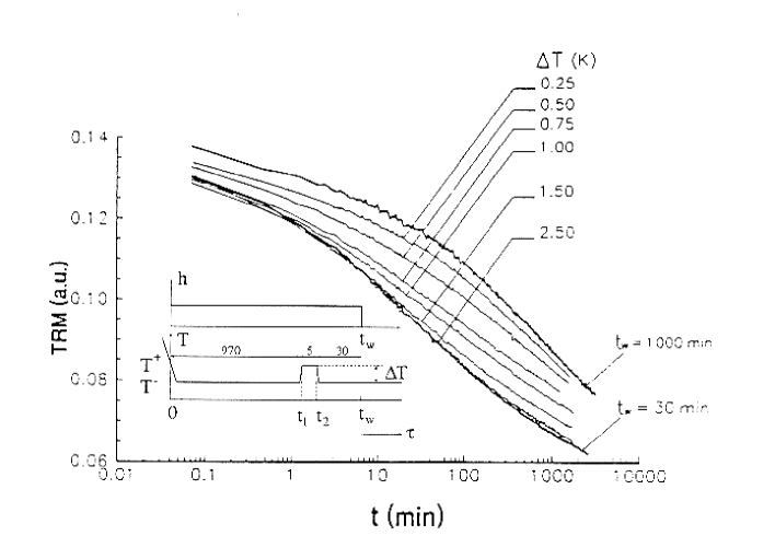
FIG. 2.: The TRM curves after a short positive cycle sketched in the inset. The relaxation is obtained at $T=12K=0.72\,T_{g}$. The bold lines are reference curves obtained after isothermal waiting at $12K$ for $t_{w}=30,\,1000$ min. The thin lines are the decay of the TRM after a cycle of $5$ min and $\Delta T=0.25,\,0.5,\,0.75,\,1,\,1.5,\,2.5\,K$. Data is courtesy of E. Vincent, see Ref. [2].

The real surprise appears when a cycle of positive temperature (inset of Fig. 2) is applied to spin glasses. Here the procedure is the inverse: the system is quenched to a temperature $T^{-}$ up to a long time $t_{1}$. This is followed by a short period at temperature $T^{+}$ from $t_{1}$ to $t_{2}$, at which $T^{-}$ is restored. As before, the field is cut off at a later time $t_{w}$ and the subsequent decay of the TRM is recorded.

The result is shown in Fig. 2. The higher the upward pulse in temperature, the generally younger the system seems but, unlike in the negative cycling case, the effect cannot be described with an effective waiting time.

Note that in the simplest cases of aging through activated processes (as for example the coarsening of the random field Ising model) the effect would be the reverse: the temperature pulse would quicken the activated processes and help aging. Refreshment would arise only if the temperature pulse is high enough to take the system above the transition.

Indeed, the solution for mean-field spin-glasses discussed below involves an additive separation of the TRM curve $M^{\sc trm}=M^{\sc rep}+M^{\sc f}$. In the positive temperature cycling the “slow” component $M^{\sc rep}$ is not affected by the pulse while the “fast” component $M^{\sc f}$ is taken to its effective critical temperature and is thus completely reinitialised. The amplitude of $M^{\sc f}$ ($M^{\sc rep}$) is larger (smaller) for higher (lower) temperature pulses. In the negative temperature cycling one is essentially probing only the slow component $M^{\sc rep}$ that is slowed down by the effect of the lower temperature excursion.

We shall show that the difference in the effects of positive and negative temperature changes is present in the mean-field version of spin-glass models while it is absent in the models thought to be a mean-field caricature of structural glasses. The relevant difference between these models resides in their dynamic behaviour below the transition. The former decay in infinitely many time-scales while the latter do in only two. (For an unambiguous definition of time-scales in aging problems see Ref. [[16]].) The explanation we give here is based on this difference. We choose to discuss in detail the magnetization behaviour although the susceptibility data, in particular the reinitialization after a negative jump, can also be understood within this framework.

Another common way to test the dynamics in the glassy phase is to apply magnetic field steps during aging at constant temperature. In these experiments no important difference is obtained between switching on and switching off the dc field. We shall briefly discuss this result within the same analytic framework.

The organisation of the paper is the following. In Section I the main features of the analytic approach are described. In Section II the temperature cycling experiments are explained within this analytic approach. The results of field cycling experiments are confronted to this approach in Section III. Section IV is devoted to some new experimental proposals and Section V to the conclusions.

I Theoretical approach

In order to understand the effect of temperature cyclings on the relaxation of the TRM and out of phase susceptibility of mean-field spin-glass models we have to understand the time-dependence of the auto-correlation and response functions:

$$C(t,t^{\prime})\equiv\frac{1}{N}\,\sum_{i=1}^{N}\langle\overline{s_{i}(t)s_{i}(t^{\prime})}\rangle\;,\;\;\;\;\;\;\;\;\;\;\;R(t,t^{\prime})\equiv\left.\frac{1}{N}\,\sum_{i=1}^{N}\frac{\delta\langle\overline{s_{i}(t)}\rangle}{\delta h_{i}(t^{\prime})}\right|_{h=0}\;.$$ (1)

For mean-field models, one obtains a set of coupled equations that entirely determine the dynamics of these two-point functions. The thermoremanent magnetization $M^{\sc trm}(t,t_{w})$ at time $t$, after cutting off a small field at time $t_{w}$, is then expressed in terms of the integrated susceptibility $\chi(t,t_{w})$:

$$\chi(t,t_{w})=\int_{t_{w}}^{t}d\tau\,R(t,\tau)\;,\;\;\;\;\;M^{\sc trm}(t,t_{w})=h[\chi(t,0)-\chi(t,t_{w})]$$ (2)

with $h$ the strength of the small dc field applied.

A The model

For definiteness let us consider the toy model consisting of $N$ continuous spins with a spherical constraint $\sum_{i}^{N}s_{i}^{2}(t)=N$ and a random energy $V({\mathchoice{{\hbox{\boldmath$\displaystyle s$}}}{{\hbox{\boldmath$\textstyle s$}}}{{\hbox{\boldmath$\scriptstyle s$}}}{{\hbox{\boldmath$\scriptscriptstyle s$}}}})$ correlated as $\overline{V({\mathchoice{{\hbox{\boldmath$\displaystyle s$}}}{{\hbox{\boldmath$\textstyle s$}}}{{\hbox{\boldmath$\scriptstyle s$}}}{{\hbox{\boldmath$\scriptscriptstyle s$}}}})V({\mathchoice{{\hbox{\boldmath$\displaystyle s$}}}{{\hbox{\boldmath$\textstyle s$}}}{{\hbox{\boldmath$\scriptstyle s$}}}{{\hbox{\boldmath$\scriptscriptstyle s$}}}^{\prime}})}=N\nu({\mathchoice{{\hbox{\boldmath$\displaystyle s$}}}{{\hbox{\boldmath$\textstyle s$}}}{{\hbox{\boldmath$\scriptstyle s$}}}{{\hbox{\boldmath$\scriptscriptstyle s$}}}}\cdot{\mathchoice{{\hbox{\boldmath$\displaystyle s$}}}{{\hbox{\boldmath$\textstyle s$}}}{{\hbox{\boldmath$\scriptstyle s$}}}{{\hbox{\boldmath$\scriptscriptstyle s$}}}^{\prime}}/N)$. The statics[18] as well as the constant temperature dynamics of this model have been solved in all detail (see Refs. [[19, 20, 21]]). Two types of models with potential correlations such that $1/\sqrt{\nu^{\prime\prime}(C)}$ is, for all $0\leq C\leq 1$, concave (convex) yield very different statics[18] (one step replica symmetry breaking versus full replica symmetry breaking) and dynamics[20] (first order versus second order dynamical transitions) and correspond to mean-field versions of structural and spin glasses respectively. Examples that have been extensively studied in the literature are the “$p=3$ spherical model” for glasses,[19] with $\nu(C)=1/2C^{3}$ (and $(\nu^{\prime\prime}(C))^{-1/2}$ concave) and the “$p=2$ plus $p=4$ model” for spin-glasses,[22] with $\nu(C)=1/2(c_{1}C^{2}+c_{2}C^{4})$ and $c_{1}$ and $c_{2}$ two constants such that $(\nu^{\prime\prime}(C))^{-1/2}$ be convex.

The exact equations of motion for $C$ and $R$ at times $t>t^{\prime}$ are [21]

$$\frac{\partial C(t,t^{\prime})}{\partial t} = -z(t)\,C(t,t^{\prime})+\int_{0}^{t^{\prime}}d\tau\,D[C(t,\tau)]\,R(t^{\prime},\tau)+\int_{0}^{t}d\tau\,\Sigma[C(t,\tau)]\,C(\tau,t^{\prime})\;,$$ (3)

$$\frac{\partial R(t,t^{\prime})}{\partial t} = -z(t)\,R(t,t^{\prime})+\int_{t^{\prime}}^{t}d\tau\,\Sigma[C(t,\tau)]\,R(\tau,t^{\prime})\;,$$ (4)

$$z(t) = T(t)+\int_{0}^{t}d\tau\;\left(D[C(t,\tau)]R(t,\tau)+\Sigma[C(t,\tau)]C(t,\tau)\right)\;,$$ (5)

with $\Sigma(t,\tau)\equiv D^{\prime}[C(t,\tau)]R(t,\tau)$, $D^{\prime}[C]=\partial_{C}D[C]$ and $D[C]=\nu^{\prime}(C)$. The function $z(t)$ is a Lagrange multiplier that enforces the spherical constraint. We shall concentrate on the spin glass-like case that corresponds to a concave random energy correlation. We shall briefly discuss the structural glass-like case at the end of this Section and explain why it does not show large asymmetry effects. Let us recall the constant temperature solution for the mean-field spin-glass models.

One of the salient features of the relaxation of mean-field spin-glasses below the dynamic critical temperature $T_{d}$ is the presence of infinitely many (two-time) scales organised in a hierarchical way. In the low temperature phase the two-point correlation and response depend on the two times involved. The form of the relaxation is usually analyzed by looking at these functions at fixed (but large) waiting time in terms of the time difference $\tau=t-t_{w}$. The correlation and response functions have a first fast stationary relaxation; for instance, the correlation rapidly decays from $1$ to $q_{EA}$, the Edwards-Anderson parameter. This time-scale is usually called the FDT regime, for reasons that will become clear below. For longer time-differences the relaxation continues at a waiting-time dependent speed. Furthermore, if one imagines the subsequent decay of the correlation as taking place in infinitesimal steps, each step takes much longer than the previous one. Indeed, in the limit of large waiting time each infinitesimal step implies a period of time that is infinitely longer than the previous one and these time-scales get completely separated. The same separation of time scales characterizes the decay of the response.

The sharp separation of time-scales allows us to split the correlations in a fast part $C^{\sc f}(t,t^{\prime})$, going from one at equal times to $q_{0}$ at very distant times, and a slow part $C_{q_{0}}(t,t^{\prime})$, going from $C_{q_{0}}(t,t)=q_{0}$ and tending to zero at even more distant times. The point at which we split the correlation is chosen arbitrarily provided it satisfies $q_{0}\leq q_{EA}$. Correspondingly we separate the response in a fast and a slow part. We then have

$$C(t,t^{\prime}) = C_{q_{0}}(t,t^{\prime})+C^{\sc f}(t,t^{\prime})-q_{0}\;,$$ (6)

$$R(t,t^{\prime}) = R_{q_{0}}(t,t^{\prime})+R^{\sc f}(t,t^{\prime})\;.$$ (7)

Since $C_{q_{0}}$ ($R_{q_{0}}$) is infinitely slower than $C^{\sc f}$ ($R^{\sc f}$) their time evolution can be characterized as follows: for all times such that $C^{\sc f}$ changes $C_{q_{0}}$ is just constant and equal to $q_{0}$. Instead, in the time-regime in which $C_{q_{0}}$ varies $C^{\sc f}$ has achieved its asymptotic value $q_{0}$ and does not further evolve.

Note that the time-scale separation is achieved only in the large waiting-time limit. This is the crucial ingredient for the argument we shall use to show that Eqs. (3)-(5) capture the phenomenology of temperature cyclings. We believe that the effects disussed in the Introduction have not been clearly observed numerically because the times explored were inevitably very short and the time-scales could not be sufficiently separated.[24, 25, 26]

As we shall show, the change in time-dependence of the fast and slow parts of $C$ and $R$ under a temperature jump are very different. The slow parts $C_{q_{0}}$ and $R_{q_{0}}$ are modified through a smooth time-reparametrization. The fast parts $C^{\sc f}$ and $R^{\sc f}$ behave as the correlation and response of an effective model with a critical temperature precisely equal to $T^{+}$. The temperature jumps have a strong effect on the fast parts and this effect is very different depending on the sign of the change.

The other salient feature of the low-temperature dynamics of mean-field spin-glasses is the violation of the fluctuation-dissipation theorem (FDT) and, most importantly, the generalized form that the relation between correlation and response takes.

A very useful way to quantify the fluctuation-dissipation relation that holds out of equilibrium is given by the relation between the integrated response $\chi(t,t_{w})$ and the correlation $C(t,t_{w})$.[16] At fixed and large $t_{w}$, one constructs a plot of $\chi(t,t_{w})$ vs $C(t,t_{w})$ using $t$ as a parameter. This is shown in Fig. 3 for two temperatures $T^{+}$ and $T^{-}$. For each temperature the $\chi$ vs. $C$ curve consists of two parts:

FIG. 3.: Sketch of the $\chi$ vs $C$ plot. The two straight lines have slopes $-1/T^{+}$ and $-1/T^{-}$ and correspond to the FDT result. The curve is temperature independent and it is given by $(\nu^{\prime\prime}(C))^{-1/2}$. The bold segment is the part erased (created) when decreasing (increasing) the temperature. See text for more details.

• A straight line of slope minus the inverse temperature. This corresponds to the fast time regime where the FDT holds and $C$ decays from $1$ to $q_{EA}$. We call this time-regime the FDT regime.

• A curve given by

  $$f(C) = \frac{1}{\sqrt{\nu^{\prime\prime}(C)}}\;.$$ (8)

  This corresponds to the slower time-regimes where the FDT is violated and $C$ decays from $q_{EA}$ to $0$ in a waiting-time dependent manner.

For temperature $T^{+}$ the $\chi$ vs $C$ plot follows the straight line of gradient $-1/T^{+}$ from $(1,0)$ to $(q_{0},\chi_{0})$ and then the curve $f(C)$ up to $(0,\chi^{\infty})$. For temperature $T^{-}$ it is given by the straight line of gradient $-1/T^{-}$ from $(1,0)$ to $(q_{1},\chi_{1})$ and then the curve $f(C)$ up to $(0,\chi^{\infty})$. The Edwards-Anderson parameters are $q_{1}$ and $q_{0}$, respectively. The two extreme cases are $T=0$ and $T=T_{c}$ (the critical temperature). The former corresponds to a vertical line starting at $(1,0)$ that matches the curve $f(C)$ at $C=1$ and then follows it up to $(0,\chi^{\infty})$. The $\chi$ vs $C$ plot for the critical temperature is just a straight line linking $(1,0)$ and $(0,\chi^{\infty})$ with a slope $-1/T_{c}$.

The remarkable fact of this family of models is that the curved segment from $(q_{0},\chi_{0})$ to $(0,\chi^{\infty})$ is the same for the temperatures below $T^{+}$. This is not a general property of mean-field spin-glass models. It holds exactly for the family of models here considered but only approximately for the Sherrington-Kirpatrick model. In the static replica approach, the corresponding property of the function $x(q)$ is called the “Parisi-Toulouse approximation”.[23] The numerical evidence seems to show that this approximation works very well in finite dimensional spin-glasses,[28] at least within numerically accessible times.

The analytic argument we shall develop below can be most easily pictured by considering Fig. 3. The range of correlation and response values in which the system has aging dynamics is given by the curved part of the plot. On changing the temperature, the straight line corresponding to the fast relaxation moves clockwise and anticlockwise like a windshield-wiper, creating and destroying the bold segment $(q_{0},\chi_{0})\rightarrow(q_{1},\chi_{1})$, thus restarting and erasing the aging scales corresponding to this interval.

B Analysis

In the limit of large waiting times we can separate the different time-regimes as follows. The equations for the fast parts of the decay are

$$\frac{\partial C^{\sc f}(t,t^{\prime})}{\partial t} = -(z^{\sc f}(t)+{\bar{z}}(t))\,C^{\sc f}(t,t^{\prime})+\int_{0}^{t^{\prime}}d\tau\;D[C^{\sc f}(t,\tau)]\;R^{\sc f}(t^{\prime},\tau)$$ (10)

$$+\int_{0}^{t}d\tau\;\;D^{\prime}[C^{\sc f}(t,\tau)]\;R^{\sc f}(t,\tau)C^{\sc f}(\tau,t^{\prime})+\bar{z}(t)\;,$$

$$\frac{\partial R^{\sc f}(t,t^{\prime})}{\partial t} = -\,(z^{\sc f}(t)+{\bar{z}}(t))R^{\sc f}(t,t^{\prime})+\int_{t^{\prime}}^{t}d\tau\;\;D^{\prime}[C^{\sc f}(t,\tau)]R^{\sc f}(t,\tau)\;R^{\sc f}(\tau,t^{\prime})\;,$$ (11)

$$z^{\sc f}(t) = T(t)+\int_{0}^{t}d\tau\left(D[C^{\sc f}(t,\tau)]+D^{\prime}[C^{\sc f}(t,\tau)]C^{\sc f}(t,\tau)\right)\,R^{\sc f}(t,\tau)\;.$$ (12)

The equations for the slow parts of the decay are

$$small = -\left(z^{\sc f}(t)+\overline{z}(t)-\int_{0}^{t}d\tau\,D^{\prime}[C^{\sc f}(t,\tau)]R^{\sc f}(t,\tau)\right)\,C_{q_{0}}(t,t^{\prime})$$ (15)

$$+\chi^{\sc f}(t^{\prime})\,D[C_{q_{0}}(t,t^{\prime})]+\int_{0}^{t^{\prime}}d\tau\,D[C_{q_{0}}(t,\tau)]\,R_{q_{0}}(t^{\prime},\tau)$$

$$+\int_{0}^{t}d\tau\,D^{\prime}[C_{q_{0}}(t,\tau)]\,R_{q_{0}}(t,\tau)\,C_{q_{0}}(\tau,t^{\prime})\;,$$

$$small = -\left(z^{\sc f}(t)+\overline{z}(t)-D^{\prime}[C_{q_{0}}(t,t^{\prime})]\chi^{\sc f}(t^{\prime})-\int_{0}^{t}d\tau\,D^{\prime}[C^{\sc f}(t,\tau)]R^{\sc f}(t,\tau)\right)\,R_{q_{0}}(t,t^{\prime})$$ (17)

$$+\int_{t^{\prime}}^{t}d\tau\;D^{\prime}[C_{q_{0}}(t,\tau)]R_{q_{0}}(t,\tau)\;R_{q_{0}}(\tau,t^{\prime})\;,$$

$${\bar{z}}(t) = \int_{0}^{t}d\tau\;\left(D[C_{q_{0}}(t,\tau)]+D^{\prime}[C_{q_{0}}(t,\tau)]C_{q_{0}}(t,\tau)\right)\,R_{q_{0}}(t,\tau)\;.$$ (18)

The input of the slow scale on the fast one is given by the one-time quantity ${\bar{z}}(t)$. The fast scale influences the slow one through three factors: $z^{\sc f}(t)$ defined in Eq. (12), $\chi^{\sc f}(t)$ and $\tilde{\chi}^{\sc f}(t)$ defined as

$$\chi^{\sc f}(t) = \int_{0}^{t}d\tau\,R^{\sc f}(t,\tau)\;,$$ (19)

$$\tilde{\chi}^{\sc f}(t) = \int_{t}^{\infty}\,d\tau R^{\sc f}(\tau,t)\;,$$ (20)

and the last term in the parenthesis of Eqs. (15) and (17). One can eliminate the dependence on this last factor by using the relation

$$small\sim-\left(z^{\sc f}(t)+\overline{z}(t)-\int_{0}^{t}d\tau\,D^{\prime}[C^{\sc f}(t,\tau)]R^{\sc f}(t,\tau)\right)\,q_{0}+\chi^{\sc f}(t)\,D[q_{0}]+\overline{z}(t)$$ (21)

that follows from Eq. (15) evaluated at

$$t^{\prime}\to t\;\;\;\;\;\;\;\;\Rightarrow\;\;\;\;\;\;\;\;C_{q_{0}}(t,t^{\prime})\to q_{0}\;.$$ (22)

After inserting the relation (21) in Eqs. (15) and (17) one has the following set of slow equations

$$small = -\frac{1}{q_{0}}(\overline{z}(t)+\chi^{\sc f}(t)D[q_{0}])\,C_{q_{0}}(t,t^{\prime})+\int_{0}^{t^{\prime}}d\tau\;D[C_{q_{0}}(t,\tau)]\;R_{q_{0}}(t^{\prime},\tau)$$ (24)

$$+\chi^{\sc f}(t^{\prime})D[C_{q_{0}}(t,t^{\prime})]+\int_{0}^{t}d\tau\;\;D^{\prime}[C_{q_{0}}(t,\tau)]R_{q_{0}}(t,\tau)\;C_{q_{0}}(\tau,t^{\prime})\;,$$

$$small = -\,\frac{1}{q_{0}}(\overline{z}(t)+\chi^{\sc f}(t)D[q_{0}])R_{q_{0}}(t,t^{\prime})+\tilde{c}hi^{\sc f}(t^{\prime})D^{\prime}[C_{q_{0}}(t,t^{\prime})]R_{q_{0}}(t,t^{\prime})$$ (26)

$$+\int_{t^{\prime}}^{t}d\tau\;D^{\prime}[C_{q_{0}}(t,\tau)]R_{q_{0}}(t,\tau)\;R_{q_{0}}(\tau,t^{\prime})\;,$$

together with Eq. (18) for $\overline{z}(t)$. The effect of the fast scales on the slow one is then only given by $z^{\sc f}(t)$, $\chi^{\sc f}(t)$ and $\tilde{\chi}^{\sc f}(t)$.

At constant temperature the quantities ${\bar{z}}(t)$, $\chi^{\sc f}(t)$ and $\tilde{\chi}^{\sc f}(t)$ tend to the following limits

$${\bar{z}}(t)\rightarrow{\bar{z}}^{\infty}\;,\;\;\;\;\;\;\;\;\chi^{\sc f}(t)\rightarrow\chi_{0}\;,\;\;\;\;\;\;\;\;\tilde{\chi}^{\sc f}(t)\rightarrow\chi_{0}\;.$$ (27)

As a consequence of the independence of temperature of $\chi(C)$ if $C<q_{EA}$, see Fig. 3, neither ${\bar{z}}^{\infty}$ nor $\chi_{0}$ depend on the temperature.

Consider now the temperature cycling experiment. We consider the effect on the slow and fast parts separately and denote the correlation after the cycle

$$C^{\sc cycle}(t,t^{\prime})=C^{\sc rep}_{q_{0}}(t,t^{\prime})+\hat{C}^{\sc f}(t,t^{\prime})\;.$$ (28)

The first term is the slow part while the second is the fast part. Similarly, for the TRM:

$$M^{\sc cycle}(t,t^{\prime})=M^{\sc rep}_{q_{0}}(t,t^{\prime})+\hat{M}^{\sc f}(t,t^{\prime})\;.$$ (29)

Under the assumption that in the presence of the cycling $C_{q_{0}}$ and $R_{q_{0}}$ are still slower than $C^{\sc f}$ and $R^{\sc f}$ and are affected at most by time-reparametrisations, an assumption whose consistency has to be checked, ${\bar{z}}(t)$ remains constant and equal to ${\bar{z}}^{\infty}$ throughout the cycle. The function $\chi^{\sc f}(t)$ stabilises to the temperature-independent value $\chi_{0}$ soon after each temperature change on a time-scale that is very short compared to any aging times since it is the relaxation of a one time-quantity.[30] Apart from a short pulse, proportional to $\chi(t)-\chi_{0}$, the slow equation feels the effect of the temperature cycling only through the small matching terms, that we collected on the left-hand-side of Eqs. (15) and (17) under the name of “small”. These affect only reparametrizations,[21] consistently with the initial assumption in the discussion.

Hence, the slow parts of the correlation and response are modified by the cycling through a smooth change in the speed of evolution, i.e. a time-reparametrisation. This is more precisely stated by studying the change of the slow parts in each time-scale. With this purpose, let us denote $C_{\alpha}^{T^{+}}(t,t^{\prime})$ and $R_{\alpha}^{T^{+}}(t,t^{\prime})$ the correlation and response function in the time-scale labelled $\alpha$ for a system aging at constant temperature $T^{+}$. In the presence of a temperature cycle between $t_{1}$ and $t_{2}$ each of these is modified according to

$$C^{\sc cycle}_{\alpha}(t,t^{\prime})=C_{\alpha}^{T^{+}}(h_{\alpha}(t),h_{\alpha}(t^{\prime}))\;,\;\;\;\;\;\;R^{\sc cycle}_{\alpha}(t,t^{\prime})=\partial_{t^{\prime}}{h_{\alpha}}(t^{\prime})\;R_{\alpha}^{T^{+}}(h_{\alpha}(t),h_{\alpha}(t^{\prime}))\;.$$

Though the calculation of $h_{\alpha}(t)$ is beyond our analytical means, we know that it has three distinct behaviours depending on the relation between $t^{\prime}$, $t$ and $t_{1}$, $t_{2}$. Obviously, $h(t)=t$ if $t<t_{1}$; $h_{\alpha}(t)$ has inflections around $t_{1}$ and $t_{2}$; and we expect $\partial_{t}h_{\alpha}(t)\sim 1$ for $t\gg t_{2}$ when the system forgot the cycle, in accordance with the weak long-term memory property.[19, 21] Furthermore, we expect that during the period $t_{1}<t<t_{2}$ the dynamics slows down, $\partial_{t}h_{\alpha}(t)<1$, if we cool down the sample, while the dynamics accelerates, $\partial_{t}h_{\alpha}(t)>1$, if we heat the sample. In Eq. (28) we have generically denoted the reparametrized slow part $C_{q_{0}}^{\sc rep}$.

The fast equations (10)-(12) decouple from the slow equation and correspond to an effective model in a constant field, since one can check that the (essentially constant) term $\overline{z}(t)$ that appears in the fast equation can be looked upon as the effect of an effective magnetic field. In fact, $T^{+}$ is the critical temperature of the model in the presence of such a field.

The temperature of the effective fast model is cycled following any of the two experimental protocols between its subcritical temperature $T^{-}$ and its critical temperature $T^{+}$. This is why the effect of the temperature change is stronger on the fast part of the correlations and heavily depends on the sign of the change.

The structural-glass models in which $(\nu^{\prime\prime}(C))^{-1/2}$ is concave have a quite simpler isothermal dynamic behaviour below its transition. They decay in only two two-time scales with a first stationary decay towards $q_{EA}$ and a subsequent slower non-stationary decay towards zero. For these models we are not allowed to separate the correlation and response in the additive way proposed in Eq. (7) for any $q_{0}$ and all the analysis presented in this seccion simply does not apply.

II Comparison with the experimental results

Let us now discuss the experimental TRM curves in the light of these results.

A Negative temperature cycling

The straight line in the $\chi$ vs. $C$ curve presented in Fig. 3 moves clockwise and then anti-clockwise to its original position. At the end of the cycle the bold part of the curve disappeared from the $\chi$ vs $C$ plot. At $t=0$ the fast model is quenched down to its critical temperature $T^{+}$, and rapidly equilibrates. At time $t_{1}$ it is further quenched to its subcritical temperature $T^{-}$ and starts aging with the effective waiting time $t_{w}^{\sc eff}=t_{w}-t_{1}$. Finally, at time $t_{2}$ the fast model is brought again to the critical temperature $T^{+}$, and it rapidly reequilibrates. The fast part has only made an excursion into its glassy phase through its quench to $T^{-}$ but, since it has been taken back to its critical temperature $T^{+}$, it has quickly forgotten it.[17]

One concludes that there is then an effective waiting-time $t_{w}^{\sc eff}$

$$t_{1}+t_{w}-t_{2}\leq t_{w}^{\sc eff}(\Delta T,t_{1},t_{2},t_{w})\leq t_{w}$$ (30)

that characterizes the evolution of the whole system, with the time spent in the lower temperature partially contributing to $t_{w}^{\sc eff}(\Delta T,t_{1},t_{2},t_{w})$.

Since the effects of negative cooling cycles are small, the fraction of time spent at $T^{-}$ needs to be rather large to observe them. Fig. 1 displays a set of curves measured after performing negative temperature cyclings of different magnitude (thin lines) and compares them to four isothermal curves associated to smaller waiting times. It is clear from the figure that the curves associated to each temperature cycling can be completely superposed to a reference isothermal curve (compare, for example, the curve for $\Delta T=T^{-}-T^{+}=-0.3K$, $t_{1}=15$ min, $t_{2}=1015$ min and $t_{w}=1030$ min with the isothermal curve for $t_{w}=100$ min). The system kept a memory of the evolution during $t_{1}$ when the temperature is raised back to its original value $T^{+}$. The time spent at the low temperature has a partial effect. There is an effective waiting time $t_{w}^{\sc eff}$ for the full system that verifies Eq. (30). The effective waiting time $t_{w}^{\sc eff}$ decreases when one cools down the system to a lower temperature until the effect of the time spent at the lower temperature becomes completely negligeable. In the experimental curves this happens for $\Delta T=-1K$. In this case, the effective aging time is simply $t_{w}^{\sc eff}=t_{1}+t_{w}-t_{2}=30$ min.

B Positive temperature cycling

In this case the straight line in Fig. 3 moves first anti-clockwise and then clockwise, exposing at the end of the cycle the bold segment of the curve.

As already discussed, the slow part of the correlation is only modified by a time-reparametrization and, since the temperature excursion has a short duration, it is hardly affected at all.

The protocol is, from the point of view of the fast model, as follows: at time $t=0$ it is quenched to a subcritical temperature $T^{-}$ and let age until $t_{1}$. At this time it is taken to its critical temperature $T^{+}$ until time $t_{2}$, fully reinitializing its age. Finally, it is quenched again into its glassy phase at time $t_{2}$ and it starts aging again. It is then clear that the fast model has an age $t_{w}^{\sc eff}=t_{w}-t_{2}<t_{w}$.

The observed TRM curves are then a superposition of a slow part, which is essentially unaffected by the temperature cycle, plus a fast part that is completely reinitialized. The relative magnitude of fast and slow parts depends upon the height of the positive excursion. Thus, for given $T^{-}$, the larger $T^{+}$ the faster the total decay of the TRM as shown in Fig. 2 where the TRM curves for temperature cyclings of the same duration but different heights are displayed.

Having the whole decay of the TRM curves as a function of the time-difference $t-t_{w}$ one can discuss them in great detail. One easily notices from the curves in Fig. 2 that one cannot associate an effective waiting time to the full TRM decay after the cycling, consistently with the the additive solution obtained analytically for the rejuvenation process.

Within the analytic framework, the larger the temperature $T^{+}$, the smaller the $q_{0}$ and $C_{q_{0}}$, implying that the fast part of the correlation and response that is completely refreshed (and hence the total rejuvenation) is larger, as we see in Fig. 2.

It has been stressed[6] that the TRM curve after a positive temperature cycle at first coincides with the isothermal TRM curve of waiting time $t_{w}\sim t-t_{2}$, the difference only becoming manifest after rather long times. If one compares the TRM curves in Fig. 2 for several values of $T^{+}$ with the isothermal curve for $t_{w}=30$ min, one observes that the departure from this reference curve is achieved later for the larger $T^{+}$s.

This is precisely what we would expect from the many-scales picture: Two protocols with the same $T^{-}$ and slightly different high temperatures $T^{+}$ and $T^{+^{\prime}}$ (associated with $q_{0}$ and $q_{0}^{\prime}$) will differ in the refreshment of the scales of $C$ and $M$ with $q_{0}<C<q_{0}^{\prime}$, and these are slower the smaller $q_{0}$. Hence, the difference in TRM between the two protocols will only show up at long times, the higher $T^{+}$.

This effect should become more and more marked for longer experiments.

III Field Cyclings

Field cyclings at constant temperature are known to yield rather large reinitializations in the out of phase susceptibility both on increasing and on decreasing the field.[32] Although we have not done a full analysis for the field cycling experiments, we may hint the reason why the arguments we used to justify a large asymmetry in temperature jump experiments do not carry through unaltered to the field cycling case.

The effect of a time-dependent field $h(t)$ on the dynamic equations is to add a term

$$A(t,t^{\prime})=h(t)\int_{0}^{t^{\prime}}d\tau\,h(\tau)R(t^{\prime},\tau)$$ (31)

to Eq. (3), and a term $A(t,t)$ to Eq. (5). In the constant field situation, these terms have the effect of eliminating the slowest scales. The $\chi$ vs $C$ plot of Fig. 3 for a constant field $h$ coincides with the one for $h=0$ but terminates at an $h$-dependent point $(q_{0},\chi_{0})$. The most outstanding effect of switching on (switching off) a field is then to erase (create) the slowest scales between $(0,\chi^{\infty})$ and $(q_{0},\chi_{0})$. Note that this is already very different from the effect of temperature changes that mainly affect the fastest scales in the problem.

One could then ask if a system that has been evolving at zero field and is suddendly taken to finite $h$ does preserve the fast parts $C^{\sc f}$ and $R^{\sc f}$ without reinitialization (just the mirror image of what an increase of temperature does). In fact, we can propose that such a solution exists, and see where the argument takes us. We hence assume a separation into a fast and a slow parts of the correlation and response just as in Eq. (7) with the value $q_{0}$ chosen to be the smallest possible correlation for a field $h$.

If we now assume that on turning on the field the fast evolution remains essentially unaltered, while the slow evolution in $C_{q_{0}}$ remains slow and finally tends to $q_{0}$ (as in a constant field case), we can separate out the fast part. The fast equations so obtained are just like Eqs. (10)-(12) with additional terms which (just as in the temperature cycling case happened for the slow parts) are constant up to, and long after the field jump. The difference is that now the “bump” in this otherwise constant factors and terms is no longer short-lasted with respect to the fast times, precisely because it comes from the slow equation and from the term (31), which has waiting time effects itself.

Hence, the initial assumption that a decoupled equation for the fast part could be found does not hold, at least in the manner it did for the slow parts in the temperature cycling case. The fast parts must be altered by the field cycling in an important way implying no big difference between switching on and off the field.

IV Proposal for new experimental measurements

The obvious direct way of constructing the $\chi$ vs $C$ plot is to perform independent measurements of the time-correlation of the magnetization noise $C(t,t_{w})$ and the integrated response $\chi(t,t_{w})$ at a given temperature and field. One can a posteriori check the independence on temperature and field of these curves.

If the assumption of independence of temperature and field of the $\chi$ vs $C$ curve in its aging part holds true, this curve can be simply obtained in a manner that is much more simple experimentally as it does not involve noise measurements and only ac susceptibilities. Indeed, let us define the quantity $y(T,h)$ as follows

$$y(T,h)\equiv\lim_{\omega\to 0}\lim_{t_{w}\to\infty}\chi^{\prime}(\omega,t_{w})=\frac{q_{d}-q_{EA}(T)}{T}\;.\;$$ (32)

The Edwards-Anderson parameter $q_{EA}(T)$ would be then independent of the field $h$ below the de Almeida-Thouless line (or “pseudo de Almeida-Thouless line” if it is only a dynamic crossover) and

$$y(T,h)=y(T)\;.$$ (33)

The parameter $q_{d}$ corresponds to

$$q_{d}\equiv\lim_{T\to 0}q_{EA}(T)\;.$$ (34)

Equation (33) can be easily checked experimentally.

Another related test is to measure the dc susceptibility

$$\chi^{\infty}(T,h)=\lim_{t_{w}\rightarrow\infty}\lim_{t\rightarrow\infty}\chi(t,t_{w})$$ (35)

at constant field $h$, presumably obtainable from the field-cooled experimental data,[33] and check if it is independent of temperature everywhere below the (pseudo) Almeida-Thouless line. There is quite a bit of evidence in this direction in the literature.[34]

One can then extract the curved part of the $\chi$ vs $C$ plot of Fig. 3, that we called $f(C)$ from the set of equations

$$C = q_{d}-Ty(T)\;,$$ (36)

$$f(C) = y(T)\;,$$ (37)

using $T$ as a parameter.

Once (and if) the validity of the approximation is verified, one can use the $\chi$ vs $C$ plot so obtained to check the consistency of the present reasoning for the cycling experiments. For example, in the positive cycling experiments the difference in TRM between the isothermal and the cycled experiment just after the cycle should be equal to the difference in height in the $\chi$ vs $C$ plot of the intersection of the straight lines corresponding to $T^{-}$ and $T^{+}$ (this is best seen by looking at Fig. 3). This non-trivial relation can be checked experimentally.

V Conclusions

While it is gratifying to be able to reproduce the qualitative experimental features analytically, we believe one should not hasten to declare that this is evidence for the mean-field scenario holding strictly. Thus, infinitely separated time-scales could in real life be just very separated scales, the Almeida-Thouless line could be just a dynamic crossover, etc.

The derivation in this paper is the first one done for a microscopic model that on one hand captures the main features of the experiments and on the other hand demonstrates the difference in the behaviour of glasses and spin-glasses. Although our calculation has relied on a particular model we believe that it will carry through to all classical mean-field spin-glass models.

There is however a problem. A satisfying scaling of the (isothermal) experimental susceptibility and TRM data simultaneously was presented in Ref. [[29]]. Surprisingly enough, this scaling has only two time-regimes as opposed to the many time-scales that we here invoked to reproduce analytically the experimental results for temperature cyclings within mean-field. If the scaling used in Ref. [[29]] turns out to hold for all times then the hierarchical scenario would not apply and some drastic modification of the present understanding must be envisaged.

- [1] L. C. E. Struick, Physical Aging in Amorphous Polymers and Other Materials (Elsevier, Houston, 1978).
- [2] P. Refregier, E. Vincent, J. Hammann and M. Ocio; J. Phys. (Paris) 48, 1533 (1987).
- [3] L. Lundgren, P. Svedlindh and O. Beckmann, J. of Magn. Magn. Mat. 31-34, 1249 (1983). P. Grandberg, L. Sandlung, P. Nordblad, P. Svendlindh, L. Lundgren, Phys. Rev. B38, 7097 (1988).
- [4] M. Lederman, R. Orbach, J. Hammann, M. Ocio and E. Vincent, Phys. Rev. B44, 7403 (1991). J. Hammann, M. Lederman, M. Ocio, R. Orbach and E. Vincent, Physica A185, 278 (1992). F. Lefloch, J. Hammann, M. Ocio and E. Vincent, Europhys. Lett. 18, 647 (1992).
- [5] L. Sandlund, P. Svedlindh, P. Granberg, P. Nordblad and L. Lundgren; J. Appl. Phys. 64, 5616 (1988). P. Granberg, L. Lundgren and P. Nordblad; J. Magn. Magn. Mater. 92, 228 (1990).
- [6] J. Hammann, F. Lefloch, E. Vincent, M. Ocio and J-P Bouchaud; in Random magnetism and high-temperature superconductivity, Beyermann, Huang-Liu and Mac Laughlin eds. (World Scientific, 1994). E. Vincent, J-P Bouchaud, J. Hammann and F. Lefloch; Philos. Mag. B71, 489 (1995).
- [7] C. Djurberg, K. Jonason and P. Nordblad, cond-mat/9810314. T. Jonsson, K. Jonason and O. Nordblad, cond-mat/9810160.
- [8] P. Doussineau, A. Levelut and Ziolkiewicz; Europhys. Lett. 33, 391 (1996); ibid, 539 (1996). F. Alberici, P. Doussineau and A. Levelut, J. Phys. 7 329 (1997). F. Alberici-Kious, J.P. Bouchaud, L.F. Cugliandolo, P. Doussineau and A. Levelut; Phys. Rev. Lett. 81, 4987 (1998).
- [9] R. L. Leheny and S. Nagel; Phys. Rev. B57, 5154 (1998).
- [10] Experiments in dipolar glasses[8] display an “intermediate” behaviour in the sense that temperature cyclings provoke strong asymmetric results, as in spin-glasses, while they also present very strong dependences on the cooling rate, a property that is not observed in spin-glasses though is very common in structural glasses.
- [11] W. L. McMillan; J. Phys. C17, 3179 (1984); Phys. Rev. B31, 340 (1985). A. J. Bray and M. A. Moore; J. Phys. C17, L463 (1984) and in Heidelberg Colloquium on Glassy Dynamics, Lecture Notes in Physics 275, ed. J. L. van Hemmen and I. Morgenstern (Springer, Berlin). D. S. Fisher and D. Huse; Phys. Rev. Lett. 56, 1601 (1986); Phys. Rev. B38, 373 (1988). G. Koper and H. Hilhorst; J. Phys. (France) 49, 429 (1988).
- [12] Vik. Dotsenko, M. Feigel’man and L. Ioffe; Spin Glasses and Related Problems, Soviet Scientific Reviews 15, (Harwood, 1990).
- [13] P. Sibani and K.H. Hoffmann; Europhys. Lett. 4, 967 (1987), Phys. Rev. A38, 4261 (1988), Europhys. Lett. 16, 423 (1991).
- [14] K.H. Hoffmann and P. Sibani; Z. Phys. B80, 429 (1990). C. Schulze, K.H. Hoffmann and P. Sibani; Europhys. Lett. 15, 361 (1991). P. Sibani, C. Uhlig and K. H. Hoffmann; Z. Phys. B95, 409 (1995). K.H. Hoffmann, S. Schubert and P. Sibani; Europhys. Lett. 38, 613 (1997). P. Sibani and K.H. Hoffmann; Physica A234, 751 (1997).
- [15] J-P Bouchaud; J. Phys. I (France) 2, 1705 (1992). J-P Bouchaud and D. S. Dean; J. Phys. I (France) 5, 265 (1995).
- [16] L. F. Cugliandolo and J. Kurchan; J. Phys. A27 (1994) 5749.
- [17] The small reinitialization effects seen in this case correspond to the re-equilibration of a critical model, and are thus very brief.
- [18] M. Mézard and G. Parisi; J. Phys. I (France) 1, 809 (1991).
- [19] L. F. Cugliandolo and J. Kurchan; Phys. Rev. Lett. 71, 173 (1993).
- [20] S. Franz and M. Mézard; Physica A209 (1994) 1. L. F. Cugliandolo and P. Le Doussal; Phys. Rev. E53, 1525 (1996).
- [21] J-P Bouchaud, L. F. Cugliandolo, J. Kurchan and M. Mézard; Out of Equilibrium dynamics in Spin-Glasses and other Glassy Systems, in Spin-Glasses and random fields, A. P. Young ed. (World Scientific, 1997); cond-mat/9702070.
- [22] T. Nieuwenhuizen; Phys. Rev. Lett. 74, 4289 (1995).
- [23] G. Parisi and G. Toulouse; J. Phys. (Paris) Lett. 41, L361 (1980).
- [24] J-O Andersson, J. Mattson and P. Svedlindh; Phys. Rev. B46, 8297 (1992).
- [25] H. Rieger; J. Phys. I (France) 4, 883 (1994). J. Kisker, L. Santen, M. Schreckenberg and H. Rieger; Phys. Rev. B53, 6418 (1996).
- [26] A. Baldassarri; cond-mat/9607162 (unpublished).
- [27] T. Komori, H. Takayama and H. Yoshino (in preparation).
- [28] E. Marinari, G. Parisi, F. Ricci-Tersenghi and J. J. Ruiz-Lorenzo; J. Phys. A31, 2611 (1998).
- [29] E. Vincent, J. Hammann, M. Ocio, J.P. Bouchaud and L. F. Cugliandolo; Slow dynamics and aging, ed. M. Rubí Sitges Conference on Glassy Systems, 1996 (springer-Verlag, in press). cond-mat/9607224.
- [30] Indeed, we have checked numerically that the full is not much affected by the temperature cycling. Changing the temperature abruptly at one sees a jump in and a later quick approach to its temperature-independent, asymptotic value. This jump is smeared out by changing the temperature with a finite velocity, as is done in experiments, and disappears if the time interval in which one changes the temperature is of the order of the FDT regime.
- [31] E. Vincent, J-P Bouchaud, D. S. Dean and J. Hammann; Phys. Rev. 52, 1050 (1995).
- [32] F. Lefloch, J. Hammann and E. Vincent, Physica B203, 63 (1994). E. Vincent, J.P. Bouchaud and J. Hammann, Phys. Rev. B52, 1050 (1995). D. Chu, G. G. Kenning and R. Orbach, Phil. Mag. B71, 479 (1995). Y. G. Joh, R. Orbach and J. Hammann, Phys. Rev. Lett. 25, 4648 (1996).
- [33] E. Vincent (private communication).
- [34] E. C. Hirschkoff, O. G. Symko, J. C. Wheatley, J. Low. Temp. Phys. 5, 155 (1977). J. L. Tholence and R. Thournier, J. Phys. Colloq. 35 C4-229 (1974). C. N. Guy J. Phys. F7, 1505 (1977). S. Nagata, P. H. Keesom, H. R. Harrison, Phys. Rev. B19, 1633 (1979). H. Aruga Katori and A. Ito, J. Phys. Soc. Japan 63, 3122 (1994).