December 1998 PAR–LPTHE 98/56

Coupled Potts models: Self-duality and fixed point structure
Vladimir Dotsenko (1), Jesper Lykke Jacobsen (2), Marc-André Lewis(1) and Marco Picco (1)

(1) LPTHE,

Université Pierre et Marie Curie, PARIS VI
Université Denis Diderot, PARIS VII
Boîte 126, Tour 16, 1^er étage
4 place Jussieu, F-75252 Paris CEDEX 05, FRANCE
(2) Laboratoire de Physique Statistique,
Ecole Normale Supérieure,
24 rue Lhomond, F-75231 Paris CEDEX 05, FRANCE

ABSTRACT

We consider $q$-state Potts models coupled by their energy operators. Restricting our study to self-dual couplings, numerical simulations demonstrate the existence of non-trivial fixed points for $2\leq q\leq 4$. These fixed points were first predicted by perturbative renormalisation group calculations. Accurate values for the central charge and the multiscaling exponents of the spin and energy operators are calculated using a series of novel transfer matrix algorithms employing clusters and loops. These results compare well with those of the perturbative expansion, in the range of parameter values where the latter is valid. The criticality of the fixed-point models is independently verified by examining higher eigenvalues in the even sector, and by demonstrating the existence of scaling laws from Monte Carlo simulations. This might be a first step towards the identification of the conformal field theories describing the critical behaviour of this class of models.
PACS numbers: 05.50.+q,64.60.Fr,75.10.Hk,75.40.Mg

1 Introduction

It is well-established that many spin models of statistical physics with random-valued nearest-neighbour couplings possess distinct critical points, their critical properties being different from those of the corresponding fixed-coupling models. To ensure the existence of a ferromagnetic-paramagnetic phase transition one usually restricts the study, within this class of models, to those where the random exchange couplings are exclusively ferromagnetic. This restriction may seem simplistic, but in fact it turns out that many models exhibiting site or bond dilution (systems where some couplings are zero), or even asymmetric distributions of positive and negative couplings, belong to the same critical universality class. Sometimes these statistical models are called “weakly disordered” in order to distinguish them from the strongly disordered models encountered in spin-glass theory, but in fact this nomenclature is somehow inappropriate, since the disorder (whose strength is here given by the spread of the distribution of random-valued couplings) could either be weak or strong. It is often observed that models with varying disorder strength display identical critical properties, a situation reminiscent of the well-known universality of the second-order phase transitions in non-disordered systems. Besides being of fundamental theoretical interest this universality is often of great practical importance: Whilst in calculations it is often simpler to consider weak randomness, in numerical studies stonger randomness is preferred, in order to reach more easily the new critical regime induced by the disorder.

An efficient laboratory for the study of disordered systems is provided by two-dimensional spin models. These models are non-trivial, critical, universal (unlike their one-dimensional counterparts) and easier to analyse, both analytically and numerically, than three-dimensional systems.

In this broad playground many results have been obtained over the years. Analytic results were mainly derived from perturbative renormalisation group calculations [1, 2, 3] whilst numerical results were obtained using Monte Carlo simulations and numerical diagonalisation of transfer matrices [4, 5, 6, 7]. Much less has been found out concerning the conformal field theories (CFTs) which should describe exactly the random systems at their critical points. This is deceiving, considering the success of CFT in describing the critical behaviour of the corresponding pure models (without disorder). Our study of coupled Potts models is mainly motivated by our interest to progress towards the identification of these conformal theories.

The relation between the two problems, coupled and random, becomes clear when one considers the replica approach to random systems. For instance, the partition function of Ising-type models with random nearest-neighbour spin couplings can be cast in the form

$$Z(\beta)=\sum_{\{\sigma\}}\mbox{exp}\left\{\beta\sum_{x,\alpha}J_{x,\alpha}\sigma_{x}\sigma_{x+\alpha}\right\}=\sum_{\{\sigma\}}\mbox{exp}\left\{-\beta\sum_{x,\alpha}J_{x,\alpha}\varepsilon_{x,\alpha}\right\}.$$ (1.1)

We can consider, for simplicity, the model on a square lattice. Then $x$ runs over the sites of the lattice and the unit vector $\alpha$ over the neighbours, $\alpha={\bf e}_{1},{\bf e}_{2}$. The couplings $J_{x,\alpha}$ assigned to links of the lattice take random values, independently for each link, with some specified distribution. The product of neighbouring spins $-\sigma_{x}\sigma_{x+\alpha}$ in Eq. (1.1) is the energy operator $\varepsilon_{x,\alpha}$ assigned to a link, which becomes a local energy operator $\varepsilon(x)$ in the continuum limit near the critical point. In this limit the partition function (1.1) can symbolically be represented as

$$Z(\beta)\propto\mbox{Tr}\,\,\exp\left\{-{\cal H}_{0}-\int d^{2}x\,m(x)\varepsilon(x)\right\},$$ (1.2)

${\cal H}_{0}$ representing the Hamiltonian (or Euclidian action, in the field theoretic terminology) of the corresponding pure CFT if it is known.

$$m(x)\propto\frac{\beta J_{x,\alpha}-\beta_{\rm c}J_{0}}{\beta_{\rm c}J_{0}},$$ (1.3)

is a mass-type coupling, which replaces $\beta J_{x,\alpha}$ in the continuum limit: the randomness of $J_{x,\alpha}$, whose average value is $J_{0}$, translates into the randomness of $m(x)$. The trace Tr in Eq. (1.3) is assumed to represent, in the continuum limit theory, the summation over the spin configurations in the lattice model (1.1).

In quenched disordered systems, averaging over the randomness should be done at the level of the free energy $F(\beta)\propto\log Z(\beta)$. To this end one introduces replicas, that is, $N$ copies of the same system

$$(Z(\beta))^{N}\propto{\mbox{Tr}}\,\,\exp\left\{-\sum^{N}_{a=1}{\cal H}^{(a)}_{0}-\int d^{2}x\,m(x)\sum^{N}_{a=1}\varepsilon_{a}(x)\right\}$$ (1.4)

and averages over the randomness:

$$\overline{(Z(\beta))^{N}}.$$ (1.5)

By taking the limit $N\to 0$ one recovers the average of the free energy for a single system:

$$\overline{F(\beta)}\propto\overline{\log Z(\beta)}\propto\lim_{N\rightarrow 0}\frac{\overline{(Z(\beta))^{N}}-1}{N}.$$ (1.6)

If the distribution of the couplings $\{J_{x,\alpha}\}$ in Eq. (1.1) is gaussian, and consequently that of $m(x)$ in Eq. (1.4), the disorder-averaged $(Z(\beta))^{N}$ in (1.5) is equivalent to a system of $N$ models coupled by their energy operators:

$$\overline{(Z(\beta))^{N}}\propto\mbox{Tr}\exp\left\{-\sum^{N}_{a=1}{\cal H}^{(a)}_{0}-m_{0}\int d^{2}x\sum^{N}_{a=1}\varepsilon_{a}(x)+g_{0}\int d^{2}x\sum_{a\neq b}\varepsilon_{a}(x)\varepsilon_{b}(x)\right\}.$$ (1.7)

Here $g_{0}$ is the width of the distribution of $m(x)$, and $m_{0}$ is its average value. At the critical point $m_{0}$ should vanish.

In cases where the distribution of $\{J_{x,\alpha}\}$, or of $m(x)$, is not gaussian, the resulting theory in Eq. (1.7) contains higher-order coupling terms, like

$$\sum_{a,b,c}\varepsilon_{a}(x)\varepsilon_{b}(x)\varepsilon_{c}(x)\qquad\mbox{and}\qquad\sum_{a,b,c,d}\varepsilon_{a}(x)\varepsilon_{b}(x)\varepsilon_{c}(x)\varepsilon_{d}(x),$$ (1.8)

but these are either irrelevant (in the renormalisation group sense) or do not modify the fixed point structure and its stability. We can thus limit our study to second order energy-energy couplings.

On the lattice, before taking the continuum limit, a similar procedure applied to $Z(\beta)$ in Eq. (1.1) produces

$$\overline{(Z(\beta))^{N}}=\sum_{\{\sigma_{a}\}}\mbox{exp}\left\{-\beta J_{0}\sum_{x,\alpha}\sum^{N}_{a=1}\varepsilon^{(a)}_{x,\alpha}+Ag_{0}\sum_{x,\alpha}\sum_{a\neq b}\varepsilon^{(a)}_{x,\alpha}\varepsilon^{(b)}_{x,a}\right\},$$ (1.9)

where $\varepsilon^{(a)}_{x,\alpha}=-\sigma^{(a)}_{x}\sigma^{(a)}_{x+\alpha}$, and $A$ is some constant coefficient.

Thus, in order to solve the random coupling problem, one first has to solve the theory of $N$ coupled homogeneous models, Eqs. (1.7) and (1.9), ultimately taking the limit $N\rightarrow 0$. A complete solution to the problem would be the identification of the exact conformal field theory associated with the critical point.

When looking for possible candidates to this conformal theory, an important issue arising is the non-unitarity of the $N\rightarrow 0$ limit theory, as can be seen using perturbative renormalisation group (RG). For instance, in a non-unitary theory the central charge increases along the RG flow, in contradistinction to what is the case for a unitary (i.e. with reflection positivity) theory [8]. As a first step, in order to avoid the problems of non-unitarity and work with a well-defined problem, we suggest to consider the problem of $N$ (positive, integer) coupled models, Eqs. (1.7) and (1.9), and to examine the critical properties of such systems. In the conformal theory language this amounts to studying $N$ minimal models, coupled two by two by the operators $\Phi_{1,2}$ which are the energy operators in the case of Ising or Potts models. This problem is unitary. The $\beta$-function of the renormalisation group, to second order in perturbation, is given by

$$\frac{dg}{d\xi}=\beta(g)\propto(N-2)g^{2}+{\cal O}(g^{3})$$ (1.10)

in the case of Ising [1], and

$$\frac{dg}{d\xi}=\beta(g)\propto 3\epsilon g+(N-2)g^{2}+{\cal O}(\epsilon^{2},g^{3})$$ (1.11)

in the case of $q$-state Potts models [2, 3], where $\epsilon\propto q-2$. By the usual analysis, for $N<2$ (and eventually for $N\rightarrow 0$) the theory (1.10) runs into zero coupling along the RG flow, and the theory (1.11) runs into a new non-trivial fixed point with

$$g_{\rm FP}\equiv g_{\ast}=\frac{3\epsilon}{2-N}+{\cal O}(\epsilon^{2}).$$ (1.12)

Thus, the random Potts model possesses a new non-trivial fixed point, and it is therefore of interest to look for the associated conformal theory.

These considerations hold true when $g$ is initially positive, that is $g_{0}>0$, which is the case for the random model. If now, in order to attain unitarity, we replace $N<2$ by $N>2$ ($N$ integer), the coefficients in Eqs. (1.10) and (1.11) change sign and the theory runs into a strong coupling regime, which is not controlled by pertubative RG and believed to be massive. This means a finite correlation length, and thus a non-critical theory.

To avoid this problem, when passing from $N<2$ to $N>2$ one should simultaneously change the sign of the initial coupling $g_{0}$. We expect some sort of similarity, or duality, of the domains $N<2,g_{0}>0$ and $N>2,g_{0}<0$. In fact, if multiplied by $(2-N)$, Eq. (1.11) takes the form:

$$\frac{d\lambda}{d\xi}\propto 3\epsilon\lambda-\lambda^{2}+{\cal O}(\lambda^{3}),$$ (1.13)

where we have defined a new coupling $\lambda=(2-N)g$. In other words, the RG flows depend on $g$ in the combination $(2-N)g$, so that the regions $N<2,g_{0}>0$ and $N>2,g_{0}<0$ are similar.

In this way one can gain unitarity whilst still staying critical. Note that the critical coupling $g_{\ast}$, Eq. (1.12), depends only on $N$ and $\epsilon(q)$. It is not obvious, but we can hope that the unitary $N>2$ problem being solved, that is the exact conformal field theory being found for general $N$, one could analytically continue into the domain $N<2$ and extract exact information about the random model, $N\rightarrow 0$.

Following this approach, we first have to find the exact conformal theory of the non-trivial fixed point $g_{\ast}$ of $N$ coupled Potts models, $N=3,4,5,...$. The first step is to study three coupled models, expecting to be able to extend the result to general $N$ later. It should be observed at this point that the model of $N$ coupled Potts lattices (minimal conformal theories) is interesting on its own right, independently of its relation to the random problem. This makes the project doubly interesting.

The system composed of three coupled $q$-state Potts models can be studied by the usual methods, in particular numerically, either by Monte Carlo simulations or by diagonalising the transfer matrix in a strip geometry. Our first objective is to get some confidence in the existence of the fixed points predicted by perturbative RG, and second, to get fairly accurate numerical values for the central charge and dimensions of operators like spin, energy and their moments $\sigma_{1}(x)\sigma_{2}(x),\,\sigma_{1}(x)\sigma_{2}(x)\sigma_{3}(x)\,$, etc. This should be useful when searching for the corresponding conformal theory.

To put the numerical study on a firm basis we need a properly defined model on the lattice, or rather on three lattices which are coupled, link to link, by their energy operators; see Eq. (1.9). For the Potts model the energy operator is of the form

$$\varepsilon_{x,\alpha}=-\delta_{\sigma_{x},\sigma_{x+\alpha}},$$ (1.14)

where $\delta_{\sigma,\sigma^{\prime}}=1$ for $\sigma=\sigma^{\prime}$ and $0$ otherwise, and the spin operator $\sigma_{x}$ at the lattice site $x$ takes $q$ different values. The partition function of three coupled models is of the form

$$\sum_{\{\sigma,\tau,\eta\}}\exp\left(\tilde{\beta}\sum_{x,\alpha}(\delta_{\sigma,\sigma^{\prime}}+\delta_{\tau,\tau^{\prime}}+\delta_{\eta,\eta^{\prime}})+\tilde{g}_{0}\sum_{x,\alpha}(\delta_{\sigma,\sigma^{\prime}}\delta_{\tau,\tau^{\prime}}+\delta_{\tau,\tau^{\prime}}\delta_{\eta,\eta^{\prime}}+\delta_{\sigma,\sigma^{\prime}}\delta_{\eta,\eta^{\prime}})\right)$$ (1.15)

with $\sigma=\sigma_{x}$ and $\sigma^{\prime}=\sigma_{x+\alpha}$ etc. In this way we have simply copied Eq. (1.9) for the particular case of $N=3$ and $a,b=1,2,3$, absorbing the coupling constant $J_{0}$ into a redefinition of $\tilde{\beta}$.

Next we have to look for critical points of Eq. (1.15), for some $\tilde{\beta}$ and negative $\tilde{g}_{0}$. If the position of the critical point is not known analytically and has to be determined numerically for a system as complicated as three coupled Potts lattices, with $q^{3}$ degrees of freedom at each site, accuracy is likely to be very poor, leading to unprecise or absurd measurements of critical properties. Thus, our numerical studies would greatly benefit from an exact determination of the position of the critical point. This can be done if the model is self-dual, like the single Ising or Potts models. For three coupled models, the existence of duality relations requires the inclusion of a three-energy interaction term

$$\sum_{x,\alpha}\delta_{\sigma,\sigma^{\prime}}\delta_{\tau,\tau^{\prime}}\delta_{\eta,\eta^{\prime}}.$$ (1.16)

In the continuum limit this becomes

$$\int d^{2}x\,\varepsilon_{1}(x)\varepsilon_{2}(x)\varepsilon_{3}(x).$$ (1.17)

It is straightforwardly shown that such a term does not modify the fixed point structure nor its stability. This means that adding (1.16) to the lattice Hamiltonian should not modify the critical properies of the model, the continuum limit theory being the same. In this way we finally arrive at a lattice model with partition function

$$\sum_{\{\sigma,\tau,\eta\}}\exp\left(\sum_{x,\alpha}\left[a\,(\delta_{\sigma,\sigma^{\prime}}+\delta_{\tau,\tau^{\prime}}+\delta_{\eta,\eta^{\prime}})+b\,(\delta_{\sigma,\sigma^{\prime}}\delta_{\tau,\tau^{\prime}}+\delta_{\tau,\tau^{\prime}}\delta_{\eta,\eta^{\prime}}+\delta_{\sigma,\sigma^{\prime}}\delta_{\eta,\eta^{\prime}})+c\,\delta_{\sigma,\sigma^{\prime}}\delta_{\tau,\tau^{\prime}}\delta_{\eta,\eta^{\prime}}\right]\right).$$ (1.18)

The coupling constants, $a$, $b$ and $c$, can be chosen so as to render this model self-dual. In Sec. 2 we shall establish the corresponding duality transformations. It will turn out that the model possesses not a point, but a line in parameter space $(a,b,c)$ on which it is self-dual. On symmetry grounds we should expect that its critical points belong to this line. In fact, it will be shown that generically there exists three self-dual fixed points:

1. That of a single Potts model with $q^{3}$ states of the spin variable. At this point $a=b=0$ and $c\neq 0$. Whenever the energy-energy coupling between the models is relevant (i.e., for $q>2$), we have $q^{3}\gg 4$. The phase transition is thus first order, and the model is not critical.

2. That of three decoupled $q$-state Potts models. At this point $b=c=0$ and $a\neq 0$. The phase transition is second order if $q\leq 4$.

3. The non-trivial fixed point of three coupled models. The transition is here second order, and the model is critical. The study of this point is the principal subject of this paper.

To make a better connection with the continuum limit theory, the energy operators of the lattice model will be redefined in the next section to take the form

$$E_{\sigma,\sigma^{\prime}}=1-\delta_{\sigma,\sigma^{\prime}}.$$ (1.19)

The principal coupling term then becomes

$$-g_{0}\sum_{x,\alpha}\left(E_{\sigma,\sigma^{\prime}}E_{\tau,\tau^{\prime}}+E_{\tau,\tau^{\prime}}E_{\eta,\eta^{\prime}}+E_{\sigma,\sigma^{\prime}}E_{\eta,\eta^{\prime}}\right),$$ (1.20)

where the parameter $g_{0}$ is a linear combination of the parameters $b,c$ in Eq. (1.18):

$$g_{0}=b+c.$$ (1.21)

With respect to $g_{0}$ the critical point 1), corresponding to a first order transition, has positive $g_{0}$, as it should have been expected. The decoupling point 2), has $g_{0}=0$, whilst the fixed point 3) is found for finite negative $g_{0}$.

As will be evident from the subsequent sections, to locate this last fixed point we have relied on the $c$-theorem of Zamolodchikov [8], which states that the effective central charge of the theory decreases along the RG flow. The effective central charge has been measured using the strip geometry, as will be explained in detail in Sec. 4. We assumed on symmetry grounds, and verified numerically, that the RG flow from the decoupling point to the non-trivial coupling point goes along the line of self-duality that we have found. To locate the point 3) we stayed on the self-dual line, on the negative $g_{0}$ side, and followed, using transfer matrices on a strip, the evolution of the effective central charge along the line. This led us to a particular limiting point on the line of self-duality, actually its end-point, at which the exact values of the couplings are known. We then used transfer matrices and Monte Carlo simulations, with the couplings tuned exactly to their end-point values, to check scaling laws and measure critical dimensions of various operators, comparing the result with those obtained by perturbative CFT.

The paper is laid out as follows. In section 2, we present duality transformations and identify the self-dual lines for two and three coupled models. Section 3 is devoted to the computation of the central charge and the critical exponents of physical operators. To this end we employ perturbative CFT techniques. Section 4 introduces the various transfer matrix algorithms we used to numerically compute the critical properties. Since these algorithms are interesting on their own right, some of them being more efficient than those previously described in the Potts model literature, they are presented extensively. Section 5 presents the numerical results obtained using these newly introduced algorithms. A Monte Carlo study of scaling laws is also undertaken. Finally, section 6 is devoted to concluding remarks and to a brief summary of the obtained results.

2 Self-duality and criticality

Duality relations, i.e. maps between sets of coupling constants that lead to the same partition functions, are central objects in the study of critical systems. These relations map one part of the coupling phase space to another one, a self-dual manifold separating the two. If the fixed points we are looking for are unique, they should be self-dual points in the phase space. If this were not the case, then fixed points would arise in dual pairs, which implies dual RG flows. Either these flows would never cross the self-dual line or they would both cross it at a given point. We are not able to picture in which way our system could behave like that. Numerical results presented later in this paper strongly support the conjecture that the fixed points of interest, for our models, are self-dual.

2.1 Duality relations

Let us first outline the construction of a global duality transformation from which the self-dual lines will be extracted. Following Ref. [10], we shall restrict our attention to Hamiltonians of the form

$${\cal H}=-\sum_{\langle i,j\rangle}J(\xi^{(1)}_{ij},\ldots,\xi^{(N)}_{ij}),$$ (2.1)

where $\xi^{(k)}_{i}=1,\ldots,q$ are the spin variables of the $k$th model and $\xi^{(k)}_{ij}\equiv|\xi^{(k)}_{i}-\xi^{(k)}_{j}|$. Energy-energy coupled Potts models naturally have Hamiltonians of this form. For generic $J$, the partition function can be written as

$$Z=\sum_{\vec{\xi}_{i}}\prod_{\langle i,j\rangle}u(\vec{\xi}_{ij}),$$ (2.2)

where $\vec{\xi}_{ij}=(\xi^{(1)}_{ij},\ldots\xi^{(N)}_{ij})$ and the local Boltzmann weights $u(\vec{\xi})$ are

$$u(\vec{\xi})=\exp\left(\beta J(\vec{\xi})\right).$$ (2.3)

The matrix $U$, whose elements are $u^{(k)}(\xi_{ij})$, is a $q\times q$ cyclic matrix. It is rather obvious that the partition function can be rewritten as

$$Z=q^{N}\sum_{\vec{\xi}_{ij}}\prod_{\langle i,j\rangle}u(\vec{\xi}_{ij}),$$ (2.4)

where a factor of $q^{N}$ has been pulled out in front, since after setting all the $\xi_{ij}$s, one still needs to fix the absolute value of one spin in each model in order to completely specify the configuration. Using Fourier transform the partition function can be defined on the dual lattice. Since it is translationally invariant, the eigenvalues of the matrix $U$ are given by

$$\lambda(\vec{\eta})=\sum_{\vec{\xi}}\exp\left(\frac{2\pi{\rm i}\vec{\xi}\cdot\vec{\eta}}{q}\right)u(\vec{\xi}),$$ (2.5)

which implies, using inverse Fourier transform, that

$$u(\vec{\xi}_{ij})=\sum_{\vec{\eta}}T(\vec{\xi}_{i},\vec{\eta})\lambda(\vec{\eta})T^{*}(\vec{\xi}_{j},\vec{\eta}),$$ (2.6)

where

$$T(\vec{\xi},\vec{\eta})=q^{-\frac{1}{2}}\exp\left(\frac{2\pi{\rm i}\vec{\xi}\cdot\vec{\eta}}{q}\right).$$ (2.7)

This can be inserted in Eq. (2.2), and leads directly to

$$Z=q^{1+N-N_{\rm D}}\sum_{\vec{\eta}_{ij}=1}^{q}\prod_{\langle i,j\rangle}\lambda(\vec{\eta}_{ij}),$$ (2.8)

where $N_{\rm D}$ is the number of sites on the dual lattice. The additional factor of $q$ comes from the fact that once all the $\vec{\eta}_{ij}$ are set, one still has to define the absolute value on one site. On a self-dual lattice, such as the square, the number of spin sites on the direct lattice and on its dual are equal (neglecting boundary effects), and one thus gets

$$Z(u)=qZ(\lambda).$$ (2.9)

The transformations (2.5) are well-defined global duality transformations. From these, self-dual solutions can be extracted. Let us treat the cases of two and three coupled models separately.

2.1.1 Two models

Consider the case of two coupled models, with Hamiltonian

$${\cal H}=\sum_{\langle i,j\rangle}{\cal H}_{ij},$$ (2.10)

$${\cal H}_{ij}=-a\,(\delta_{\sigma_{i},\sigma_{j}}+\delta_{\tau_{i},\tau_{j}})-b\,\,\delta_{\sigma_{i},\sigma_{j}}\delta_{\tau_{i},\tau_{j}}.$$ (2.11)

The choice of sign for the coupling $b$ conforms with existing computations for the random model.

The duality relations, mapping the couplings $(a,b)$ to $(a^{*},b^{*})$, are given by

$${\rm e}^{2a^{*}+b^{*}} = \frac{{\rm e}^{2a+b}+2(q-1){\rm e}^{a}+(q-1)^{2}}{{\rm e}^{2a+b}-2{\rm e}^{a}+1},$$ (2.12)

$${\rm e}^{a^{*}} = \frac{{\rm e}^{2a+b}+(q-2){\rm e}^{a}-(q-1)}{{\rm e}^{2a+b}-2{\rm e}^{a}+1}.$$ (2.13)

The denominator is introduced to ensure that configurations of zero energy remain as such under duality. The self-duality condition constrains couplings $a$ and $b$ to satisfy

$${\rm e}^{b}={2{\rm e}^{a}+(q-1)\over{\rm e}^{2a}}.$$ (2.14)

Two points of direct physical interpretation can be found on this line. First, the decoupled point $b=0$ for which $a=\ln(1+\sqrt{q})$, which is the usual critical temperature $\beta_{\rm c}(q)$ of the decoupled models. The second, at $a=0$ and $b=\ln(1+q)$, corresponds to a $q^{2}$-state Potts model, for which $\beta_{\rm c}(q^{2})=\ln(1+q)$. We remark that the case of two coupled models was previously considered by Domany and Riedel [11].

2.1.2 Three models

The Hamiltonian associated with the case of three coupled models is

$${\cal H}=\sum_{\langle i,j\rangle}{\cal H}_{ij},$$ (2.15)

$${\cal H}_{ij} = -a\,(\delta_{\sigma_{i},\sigma_{j}}+\delta_{\tau_{i},\tau_{j}}+\delta_{\eta_{i},\eta_{j}})-b\,(\delta_{\sigma_{i},\sigma_{j}}\delta_{\tau_{i},\tau_{j}}+\delta_{\sigma_{i},\sigma_{j}}\delta_{\eta_{i},\eta_{j}}+\delta_{\tau_{i},\tau_{j}}\delta_{\eta_{i},\eta_{j}})$$ (2.16)

$$- c\,\,\delta_{\sigma_{i},\sigma_{j}}\delta_{\tau_{i},\tau_{j}}\delta_{\eta_{i},\eta_{j}}.$$

The introduction of a three-coupling term is necessary to produce self-dual solutions, since it is generated by applying the duality relations to our original Hamiltonian. The duality transformations are given by

$${\rm e}^{3a^{*}+3b^{*}+c^{*}} = \frac{{\rm e}^{3a+3b+c}+3(q-1){\rm e}^{2a+b}+3(q-1)^{2}{\rm e}^{a}+(q-1)^{3}}{{\rm e}^{3a+3b+c}-3{\rm e}^{2a+b}+3{\rm e}^{a}-1},$$ (2.17)

$${\rm e}^{2a^{*}+b^{*}} = \frac{{\rm e}^{3a+3b+c}+(2q-3){\rm e}^{2a+b}+(q^{2}-4q+3){\rm e}^{a}-(q-1)^{2}}{{\rm e}^{3a+3b+c}-3{\rm e}^{2a+b}+3{\rm e}^{a}-1},$$ (2.18)

$${\rm e}^{a^{*}} = \frac{{\rm e}^{3a+3b+c}+(q-3){\rm e}^{2a+b}+(3-2q){\rm e}^{a}+(q-1)}{{\rm e}^{3a+3b+c}-3{\rm e}^{2a+b}+3{\rm e}^{a}-1}.$$ (2.19)

Self-duality solutions are found to be

$${\rm e}^{b} = {(2+\sqrt{q}){\rm e}^{a}-(\sqrt{q}+1)\over{\rm e}^{2a}},$$

$${\rm e}^{c} = {\rm e}^{3a}{3({\rm e}^{a}-1)(\sqrt{q}+1)+q\sqrt{q}+1\over({\rm e}^{a}(2+\sqrt{q})-(1+\sqrt{q}))^{3}}.$$ (2.20)

The two trivial points found in the two-models case also arise here; the decoupling point, for which $b=c=0$ and $a=\ln(1+\sqrt{q})$, and the $q^{3}$-state Potts model, with $a=b=0$ and $c=\beta_{\rm c}(q^{3})=\ln(1+q^{3/2})$.

2.2 A convenient reparametrisation

There is a certain arbitrariness in the way we choose to parametrise a point on the self-dual line. Ideally, the couplings entering the lattice Hamiltonian would in some way be comparable to those of the field theory describing its continuum limit. Evidently, decoupling points should be associated with null couplings in both schemes, but this still leaves plenty of room for a reparametrisation. We propose such a reparametrisation which makes closer contact with the physical considerations put forward in the Introduction, and, at the same time, facilitates the implementation of numerical methods.

2.2.1 General case

Introducing the parameter $x$ ($x\in[1,+\infty[$) in Eq. (2.16), the self-duality relations can be rewritten as

$${\rm e}^{a} = \frac{\sqrt{q}+1}{\sqrt{q}+2}x,$$ (2.21)

$${\rm e}^{b} = \frac{(\sqrt{q}+2)^{2}}{\sqrt{q}+1}\frac{x-1}{x^{2}},$$ (2.22)

$${\rm e}^{c} = \frac{3(\sqrt{q}+1)^{2}}{(\sqrt{q}+2)^{4}}\frac{x^{3}(x-\gamma)}{(x-1)^{3}},$$ (2.23)

where $\gamma\equiv\frac{4-q}{3}$. Since the decoupled models we study have ferromagnetic ground states, it is more convenient to trade the $\delta_{\sigma_{i},\sigma_{j}}$ for the operators

$$E_{\sigma_{i},\sigma_{j}}=1-\delta_{\sigma_{i},\sigma_{j}}.$$ (2.24)

Doing so, the Hamiltonian becomes

$${\cal H}_{ij} = -(3a+3b+c)+(a+2b+c)\,(E_{\sigma_{i},\sigma_{j}}+E_{\tau_{i},\tau_{j}}+E_{\eta_{i},\eta_{j}})$$ (2.25)

$$- (b+c)\,(E_{\sigma_{i},\sigma_{j}}E_{\tau_{i},\tau_{j}}+E_{\sigma_{i},\sigma_{j}}E_{\eta_{i},\eta_{j}}+E_{\tau_{i},\tau_{j}}E_{\eta_{i},\eta_{j}})$$

$$+ c\,\,E_{\sigma_{i},\sigma_{j}}E_{\tau_{i},\tau_{j}}E_{\eta_{i},\eta_{j}}.$$

The constant term, being the ground state energy, can be gauged out. Now define the new one- and two-energy coupling constants

$$\beta = a+2b+c,$$

$$g = b+c.$$ (2.26)

With this set of couplings the Hamiltonian is turned into

$${\cal H}_{ij} = \beta\,(E_{\sigma_{i},\sigma_{j}}+E_{\tau_{i},\tau_{j}}+E_{\eta_{i},\eta_{j}})$$ (2.27)

$$- g\,(E_{\sigma_{i},\sigma_{j}}E_{\tau_{i},\tau_{j}}+E_{\sigma_{i},\sigma_{j}}E_{\eta_{i},\eta_{j}}+E_{\tau_{i},\tau_{j}}E_{\eta_{i},\eta_{j}})$$

$$+ c\,\,E_{\sigma_{i},\sigma_{j}}E_{\tau_{i},\tau_{j}}E_{\eta_{i},\eta_{j}}.$$

On the self-dual line the couplings $\beta$ and $g$ are parametrised by

$${\rm e}^{-\beta} = \frac{\sqrt{q}+2}{3(\sqrt{q}+1)}\frac{x-1}{x-\gamma},$$ (2.28)

$${\rm e}^{g} = \frac{3(\sqrt{q}+1)}{(\sqrt{q}+2)^{2}}\frac{x(x-\gamma)}{(x-1)^{2}}.$$ (2.29)

A similar reparametrisation for the case of two models leads to the Hamiltonian

$${\cal H}_{ij}=\beta(E_{\sigma_{i},\sigma_{j}}+E_{\tau_{i},\tau_{j}})-g(E_{\sigma_{i},\sigma_{j}}E_{\tau_{i},\tau_{j}}),$$ (2.30)

with

$${\rm e}^{-\beta} = \frac{x^{2}}{2x^{2}+x(q-1)},$$

$${\rm e}^{g} = \frac{2x+(q-1)}{x^{2}}.$$ (2.31)

This particular parametrisation has some definite advantages over the original one. First, all Boltzmann weights remain finite along the self-dual line, something useful both in numerical studies and in a comparison with perturbative CFT. Second, as we shall see in Sec. 3, along the self-dual line, the coupling constant $g$ has a sign in agreeement with perturbative computations. Finally, in the three-models case, the three-coupling term becomes infinite when $x\to\infty$, leading to a null Boltzmann weight. This implies some simplifications of numerical studies, as we now show.

2.2.2 Limits on the self-dual lines

As we just said, the limit $x\to\infty$ will be of special interest in the following sections. There we can simplify numerical computations (both using transfer matrices and Monte Carlo simulations) by suppressing some of the Boltzmann weights attached to the links. The local Boltzmann weight $W(L_{ij})$ for the degrees of freedom coupling spin sites $i$ and $j$ is completely determined by specifying the number $L_{ij}$ of layers having different spin values at the two ends of the bond ($ij$). The total Boltzmann weight of a spin configuration is then given by

$$W=\prod_{\langle i,j\rangle}W(L_{ij}).$$ (2.32)

If we consider the case of two coupled models, Eq. (2.30), three possible weights $W(L)$ arise:

$$W(0)=1,\ \ \ \ W(1)={\rm e}^{-\beta},\ \ \ \ W(2)={\rm e}^{-2\beta+g}.$$ (2.33)

Using the self-dual parametrised solutions, we see that in the limit $x\to\infty$ this becomes

$$W(0)=1,\ \ \ \ W(1)=1/2,\ \ \ \ W(2)=0.$$ (2.34)

For the case of three models, Eq. (2.25), there are four possible weights

$$W(0)=1,\ \ \ \ W(1)={\rm e}^{-\beta},\ \ \ \ W(2)={\rm e}^{-2\beta+g},\ \ \ \ W(3)={\rm e}^{-3\beta+3g-c}.$$ (2.35)

At $x\rightarrow\infty$ this becomes

$$W(0)=1,\ \ \ \ W(1)=\frac{\sqrt{q}+2}{3(\sqrt{q}+1)},\ \ \ \ W(2)=\frac{1}{3(\sqrt{q}+1)},\ \ \ \ W(3)=0,$$ (2.36)

We shall use this limit extensively later on. The fact that configurations with one or more $L_{ij}$ equal to three are forbidden greatly simplifies the problem. It even gives hope to solve exactly the lattice model at the critical point. In Sec. 4.5 below we shall see that it is possible to reformulate the Hamiltonians (2.30) and (2.25) so as to obtain even more null Boltzmann weights, by passing on to a random cluster picture.

3 Renormalisation group study of
coupled Potts models

Coupled Potts models have already been studied in details using renormalisation group techniques. Details can be found in references [2, 3, 12, 13, 14, 15]. We shall only present here a summary of these results, which are exposed extensively in the given references.

The continuum limit of the models under consideration is defined by

$${\cal H}=\displaystyle\sum_{i=1}^{N}{\cal H}_{0,i}-g\int d^{2}x\displaystyle\sum_{i\neq j}^{N}\varepsilon_{i}(x)\varepsilon_{j}(x),$$ (3.1)

where $\varepsilon_{i}(x)$ is the continuum limit of $E_{\sigma_{i},\sigma_{j}}$ [see Eq. (2.24)] and corresponds to the energy operator, and ${\cal H}_{0,i}$ are the Hamiltonians of the decoupled Potts models in the continuum limit. We shall restrict the discussion to $q$-state Potts models with $2\leq q\leq 4$, for which the dimension of the energy operator varies between $1$ (for $q=2$) and $1/2$ (for $q=4$). For such values of $q$, the continuum limit of the models are conformal field theories. The term $g\int\varepsilon\varepsilon$ is considered as a perturbation, which is relevant by dimensional analysis (except for $q=2$, where it is marginal). The computation of the $\beta$-function to two loops was done in Refs. [2, 3] and is given by

$$\beta(g)\equiv{dg\over d\log(r)}=3\epsilon g(r)+4\pi(N-2)g^{2}(r)-16\pi^{2}(N-2)g^{3}(r)+{\cal O}(g^{4}(r)).$$ (3.2)

Here $\epsilon$ is the perturbation parameter, and it corresponds to the dimension of the perturbation: $\epsilon=\frac{2}{3}\left(1-\Delta_{\varepsilon}\right)$ where $\Delta_{\varepsilon}$ is the dimension of the energy operator of the decoupled models. For $q=2$ we have $\epsilon=0$, whilst for $q=3$, $\epsilon=2/15$ and for $q=4$, $\epsilon=1/3$. The parameter $r$ is an infrared cut-off.

In order to compute critical exponents we need to compute the matrices $(Z_{\varepsilon})_{ij}$ and $(Z_{\sigma})_{ij}$ which are respectively the renormalisation constants of the energy and spin operators. These have to be understood in the following way:

$$\vec{\cal O}_{\rm R}=(Z_{\cal O})\vec{\cal O},$$ (3.3)

where the $i$th element of vector $\vec{\cal O}$ is the operator $\cal O$ of model $i$, and ${\cal O}_{\rm R}$ is the corresponding renormalised operator. These matrices are, again to second order in the perturbation, given by [3]

$$\frac{d\log(Z_{\varepsilon}(r))_{ij}}{dr}=\left(-4\pi(N-1)g-8\pi^{2}(N-1)g^{2}+{\cal O}(g^{3})\right)(1-\delta_{ij}),$$ (3.4)

$$\frac{d\log(Z_{\sigma}(r))_{ij}}{dr}=\left(3(N-1)g^{2}\pi^{2}\epsilon\,{\cal F}+4(N-1)(N-2)\pi^{3}g^{3}+{\cal O}(g^{4})\right)\delta_{ij},$$ (3.5)

with

$${\cal F}=2\,\frac{\Gamma^{2}(-\frac{2}{3})\Gamma^{2}(\frac{1}{6})}{\Gamma^{2}(-\frac{1}{3})\Gamma^{2}(-\frac{1}{6})}.$$ (3.6)

The fact that the energy matrix is not diagonal was observed in Refs. [2, 15]. This implies that the energy operators for each individual layer are no longer the proper ones to study critical behaviour. Instead, the eigenvectors of the matrix turn out to be the ones we observe in numerical studies. We shall come back to this point when we compute critical exponents in the next sub-section.

The possible behaviours of our coupled systems can be summarised as follows [13].

• For $q=2$ the model corresponds to the $N$-colour Ashkin-Teller model. For $N=2$ it is integrable [16]. For $N>2$ the sign of $g$ is determinant for the large-scale behaviour: When $g>0$ a second order phase transition of the Ising type is observed, whilst for $g<0$ the scenario is that of a fluctuation-driven first order phase transition [17, 18].

• For $q>2$ and $N=2$ the model is still integrable, but now presents a mass generation [19]. This again indicates a first order phase transition.

• For the case $N>2$ and $g>0$ the coupling constants flow far from our perturbative region. Even if a definite proof is not given, a comparison with the case $q=2$ seems to tell us that a mass gap is dynamically generated, indicating a first order phase transition.

  The situation is completely different for $g<0$. In that case there is a non-trivial infrared fixed point for

  $$g_{*}=-{3\epsilon\over 4\pi(N-2)}+{9\epsilon^{2}\over 4\pi(N-2)^{2}}+{\cal O}(\epsilon^{3})$$ (3.7)

  The critical exponents associated with the energy and spin operators for this fixed point, along with the values of the central charge, are computed below.

3.1 Critical exponents for $q>2,N>2$

We now compute the critical exponents of our coupled models at the fixed points of the renormalisation group. For the decoupling point, the critical exponents are evidently the ones of the pure models. We shall therefore concentrate on the non-trivial fixed point identified above. Since the renormalisation matrix for the spin operator is diagonal and the coupling is invariant under permutation, any linear combination of the spin operators has a well-defined critical exponent which is found to be [3]

$$\Delta^{\prime}_{\sigma}=\Delta_{\sigma}-\frac{27}{16}\frac{N-1}{(N-2)^{2}}\,{\cal F}\epsilon^{3}+{\cal O}(\epsilon^{4}),$$ (3.8)

where ${\cal F}$ was defined in Eq. (3.6).

Defining critical exponents for the energy operators is somehow more tricky. Correlation functions between renormalised operators (at a given cut-off $R$) are of the following form

$$\langle\varepsilon_{i}(0)\varepsilon_{j}(R)\rangle\sim\sum_{k\neq i}\sum_{l\neq j}(Z_{\varepsilon})_{ik}(Z_{\varepsilon})_{jl}\frac{1}{R^{2\Delta_{\varepsilon}}}\langle\varepsilon_{k}(0)\varepsilon_{l}(1)\rangle,$$ (3.9)

mixing correlation functions of the $N$ different layers. One way to extract unambiguous critical exponents is to diagonalise the renormalisation matrix, thus introducing a new basis of operators. This diagonalisation is exact, in the sense that eigenvectors for the one-loop renormalisation matrix remain eigenvectors to all order in the perturbation. For three models the eigenvectors are

$$\varepsilon_{1}+\varepsilon_{2}+\varepsilon_{3},\qquad\varepsilon_{1}-\varepsilon_{2},\qquad\varepsilon_{2}-\varepsilon_{3}.$$ (3.10)

When using this basis, the computation of the different exponents is straightforward. We have [15]

$$\Delta_{\varepsilon_{1}+\varepsilon_{2}+\varepsilon_{3}}=\Delta_{\varepsilon}+6\epsilon-9\epsilon^{2}+{\cal O}(\epsilon^{3})$$ (3.11)

and

$$\Delta_{\varepsilon_{1}-\varepsilon_{2}}=\Delta_{\varepsilon}-3\epsilon+\frac{9}{2}\epsilon^{2}+{\cal O}(\epsilon^{3}).$$ (3.12)

Some explicit values of the different critical exponents for the case of three coupled model are provided by Table 1. The appearance of negative magnetic exponents for sufficiently large $q$ shows the limitations of the perturbative expansion. It is also possible to compute the critical exponents for higher moments of the spin and energy operators. The physically significant operators are found to be

$$\sigma_{1}\sigma_{2},\qquad\sigma_{1}\sigma_{3},\qquad\sigma_{2}\sigma_{3},\qquad\sigma_{1}\sigma_{2}\sigma_{3};$$ (3.13)

$$\varepsilon_{1}\varepsilon_{2}+\varepsilon_{2}\varepsilon_{3}+\varepsilon_{3}\varepsilon_{1},\qquad\varepsilon_{1}\varepsilon_{2}-\varepsilon_{2}\varepsilon_{3},\qquad\varepsilon_{1}\varepsilon_{2}-\varepsilon_{3}\varepsilon_{1},\qquad\varepsilon_{1}\varepsilon_{2}\varepsilon_{3}.$$ (3.14)

As was shown for the random Potts model [20], perturbative computations for higher moments of the spin and energy operators are much less precise than for the operators themselves, and one should keep in mind that they eventually become absurd for sufficiently high moments (for example, the third magnetic moment has negative exponent for $q>3.7$). For the spin operators, the second order perturbative computations lead to the following exponents [21, 20]

$$\Delta_{\sigma_{1}\sigma_{2}}=2\Delta_{\sigma}(\epsilon)+\frac{3\epsilon}{4(N-2)}\left(1-\frac{3\epsilon}{N-2}\left((N-2)\log 2+\frac{11}{12}\right)\right)+{\cal O}(\epsilon^{3}),$$ (3.15)

$$\Delta_{\sigma_{1}\sigma_{2}\sigma_{3}}=3\Delta_{\sigma}(\epsilon)+\frac{9\epsilon}{4(N-2)}\left(1-\frac{3\epsilon}{N-2}\left((N-2)\log 2+\frac{11}{12}+\frac{\alpha}{24}\right)\right)+{\cal O}(\epsilon^{3}),$$ (3.16)

with

$$\alpha=33-\frac{29\sqrt{3}\pi}{3}.$$ (3.17)

For the energy operators, critical exponents for the diagonal operators are given by ($\varepsilon_{\rm S}^{2}\equiv\varepsilon_{1}\varepsilon_{2}+\varepsilon_{2}\varepsilon_{3}+\varepsilon_{3}\varepsilon_{1}$ and $\varepsilon_{\rm A}^{2}\equiv\varepsilon_{1}\varepsilon_{2}-\varepsilon_{2}\varepsilon_{3}$)

$$\Delta_{\varepsilon_{\rm S}^{2}} = 2\Delta_{\varepsilon}(\epsilon)+3\epsilon+\frac{9}{2}\epsilon^{2}+{\cal O}(\epsilon^{3})$$ (3.18)

$$\Delta_{\varepsilon_{\rm A}^{2}} = 2\Delta_{\varepsilon}(\epsilon)-\frac{3}{2}\epsilon-9\epsilon^{2}+{\cal O}(\epsilon^{3})$$ (3.19)

$$\Delta_{\varepsilon_{1}\varepsilon_{2}\varepsilon_{3}} = 3\Delta_{\varepsilon}(\epsilon)-\frac{27}{4}\epsilon^{2}+{\cal O}(\epsilon^{3})$$ (3.20)

The numerical values for these operators are given in Table 2.

$q$	$\Delta_{\varepsilon_{1}+\varepsilon_{2}+\varepsilon_{3}}$	$\Delta_{\varepsilon_{1}-\varepsilon_{2}}$	$\Delta_{\sigma_{1}}$
2.00	1.0000	1.0000	0.12500
2.25	1.1447	0.8499	0.12789
2.50	1.2639	0.7154	0.12964
2.75	1.3615	0.5930	0.12985
3.00	1.4400	0.4800	0.12805
3.25	1.5006	0.3737	0.12353
3.50	1.5429	0.2710	0.11501
3.75	1.5624	0.1656	0.09926
4.00	1.5000	0.0000	0.04238

Table 1: Perturbative critical exponents of physically significant energy and spin operators for three coupled $q$-state Potts models.

$q$	$\Delta_{\varepsilon_{1}\varepsilon_{2}+\varepsilon_{2}\varepsilon_{3}+\varepsilon_{3}\varepsilon_{1}}$	$\Delta_{\varepsilon_{1}\varepsilon_{2}-\varepsilon_{2}\varepsilon_{3}}$	$\Delta_{\varepsilon_{1}\varepsilon_{2}\varepsilon_{3}}$	$\Delta_{\sigma_{1}\sigma_{2}}$	$\Delta_{\sigma_{1}\sigma_{2}\sigma_{3}}$
2.00	2.000	2.000	3.000	0.2500	0.3750
2.25	2.005	1.834	2.837	0.2775	0.4553
2.50	2.021	1.653	2.664	0.2949	0.5190
2.75	2.046	1.456	2.479	0.3030	0.5685
3.00	2.080	1.240	2.280	0.3023	0.6048
3.25	2.126	0.997	2.060	0.2921	0.6283
3.50	2.186	0.713	1.806	0.2703	0.6375
3.75	2.272	0.350	1.486	0.2303	0.6268
4.00	2.500	-0.500	0.750	0.0975	0.5301

Table 2: Perturbative critical exponents of physically significant energy and spin operator moments for three coupled $q$-state Potts models.

3.2 Central charge and the $c$-theorem for $q>2,N>2$

One of the most important tools of CFT, Zamolodchikov’s $c$-theorem [8], provides a simple way of computing the central charge for perturbed theories. Moreover, it gives us crucial information:

• The $c$-function, to be defined below, is decreasing along the renormalisation flow.

• If the flow has a fixed point, the field theory at the fixed point is conformally invariant and its central charge is the value of the $c$-function at that point.

With our conventions for the $\beta$-function taken into account, the $c$-function is defined as

$$c(g^{\prime})=c_{\rm pure}-24\int_{0}^{g^{\prime}}\beta(g)\mbox{d}g,$$ (3.21)

with $c_{\rm pure}$ being the total central charge of the decoupled models. The central charge deviation from the decoupling point value is thus easily computed. Substituting $g^{\prime}=g_{*}$, the fixed point value of the couplings, we get the following correction:

$$\Delta c = -24\int_{0}^{g_{*}}\beta(g)\mbox{d}g$$ (3.22)

$$= -\frac{27}{8}\frac{N(N-1)}{(N-2)^{2}}\left(\epsilon^{3}-\frac{9}{2(N-2)}\epsilon^{4}\right)+{\cal O}(\epsilon^{5})$$ (3.23)

Table 3 presents the pure and perturbative values of the central charge. Clearly, for large enough $q$ the latter are not to be trusted, since the perturbation theory eventually breaks down. This is witnessed by the change of sign in Eq. (3.23) when $\epsilon>\frac{2}{9}$.

$q$	$c_{\rm pure}$	$c_{\rm FP}$
2.00	1.5000	1.5000
2.25	1.7627	1.7620
2.50	1.9975	1.9931
2.75	2.2089	2.1976
3.00	2.4000	2.3808
3.25	2.5734	2.5500
3.50	2.7309	2.7164
3.75	2.8734	2.9054
4.00	3.0000	3.3750

Table 3: Comparison of the central charge values at the pure and the non-trivial fixed points.

4 The transfer matrices

Systems of several coupled $q$-state Potts models possess an enormous number of states, and one should think that accurate numerical results cannot be obtained by the transfer matrix technique, since only very narrow strips can be accessed. However, there are several possibilities for dramatically reducing the size of the state space, as we show in the present Section. In particular we shall see that it is possible to numerically study the $q$-state Potts model for any real $q$ with less computational effort than is required in the traditional transfer matrix approach to the Ising model.

We have optimised the algorithm described in Ref. [5], and adapted it to the case of three coupled models, by taking into account all known symmetries of the Boltzmann weights in the spin basis. Further progress can be made by trading the spin variables for clusters or loops. The cluster algorithm of Ref. [22] has been adapted to the problem of coupled models, and we also describe, for the first time in the literature, the practical implementation of the associated loop algorithm. The latter algorithm allows us to address the case of three coupled models on strips of width $L_{\rm max}=12$.

4.1 The four algorithms

Consider a system of coupled Potts models defined on a cylinder of circumference $L$ and length $M$, measured in units of the lattice constant. The imposition of periodic boundary conditions in the transversal direction is understood throughout. The transfer matrix can be viewed as a linear operator ${\bf T}$ that acts on the partition function of the $M$ row system, where fixed boundary conditions have been imposed on the degrees of freedom of the $M$th row, so as to generate the corresponding quantity for a system with $M+1$ rows. To fix terminology, we shall refer to the specification of the boundary condition on the last row as the state of the system. Thus, symbolically,

$$Z_{\alpha}^{(M+1)}=\sum_{\beta}T_{\alpha\beta}Z_{\beta}^{(M)},$$ (4.1)

where the Greek subscripts label the possible states. The matrix elements $T_{\alpha\beta}$ are nothing but the Boltzmann factors $\exp[-{\cal H}(\alpha,\beta)]$ arising from the interaction between the degrees of freedom in the $M$th and the $(M+1)$th row, when these are in the fixed states $\beta$ and $\alpha$ respectively.

It is well-known that crucial information about the free energy, the central charge, and the scaling dimensions of various physical operators can be extracted from the asymptotic scaling (with strip width $L$) of the eigenvalue spectrum of the transfer matrix, and so the question arises what is the most efficient way of diagonalising it. A quite common trick is to decompose it as a product of sparse matrices which each add a single degree of freedom to the $M$th row, rather than an entire new row at once. But even more important is the realisation that the total number of states, and thus the dimensionality of the transfer matrix, can be reduced by taking into account the various symmetries of the interactions and possibly by rewriting the model in terms of new degrees of freedom other than simply the Potts spins. We shall refer to any such collection of states as a basis of the transfer matrix, and the cardinality of the basis as its size. The accuracy of the finite-size data, of course, improves significantly with increasing $L$, and since the size is a very rapidly (typically exponentially) increasing function of $L$ we must face the highly non-trivial algorithmic problem of identifying and implementing the most efficient basis.

These considerations have led to the development of four different algorithms for the coupled Potts models problem. We list them here in order of increasing efficiency and, roughly, increasing algorithmic ingenuity. Details on the implementations will be given in the following sub-sections. As a rough measure of their respective efficiency we indicate how large $L$ can be attained in practice for the three-layered model.

• alg1 uses the trivial basis of Potts spins and can access $L=5$ for $q=3$ and $L=4$ for $q=4$. Although hopelessly inefficient in the general case this algorithm is still of some use for small, integer $q$ since it allows for a straightforward access to magnetic properties.

• alg2 still works in the spin basis, but the $Z_{q}$ symmetry of the Potts spins has been factored out. In this process the magnetic properties are lost. The size is now independent of $q$, but for $q<L$ a further reduction of the size occurs due to a truncation of the admissible states. For $q=3$ this algorithm can access $L=7$, but for general $q$ only $L=6$.

• alg3 utilises a mapping to the random cluster model, and the basis consists of the topologically allowed (‘well-nested’) connectivities with respect to clusters of spins that are in the same Potts state. Magnetic properties are lost, but can be restored through the inclusion of a ghost site at the expense of increasing the number of basis states. Since $q$ enters only as a (continuous) parameter, this algorithm is particularly convenient for comparing with analytic results obtained by perturbatively expanding in powers of $(q-2)$. In the non-magnetic sector $L=7$ can be accessed.

• alg4 works in a mixed representation of random clusters and their surrounding loops on the medial lattice. Magnetic properties can be addressed through the imposition of twisted boundary conditions, which by duality are equivalent to the topological constraint that clusters and loops do not wrap around the cylinder. Again $q$ is a continuous parameter. Due to the definition of the medial lattice, only even $L$ are allowed. This algorithm can access $L=12$ in the non-magnetic sector and $L=10$ in the magnetic one.

Before turning our attention to a detailed description of these algorithms we briefly recall how physically interesting quantities may be extracted from the transfer matrix spectra.

4.2 Extraction of physical quantities

The reduced free energy per spin in the limit $M\to\infty$ of an infinitely long cylinder is given by

$$f_{0}(L)=-\lim_{M\to\infty}\frac{1}{LM}\ln{\rm Tr}Z^{(M)}=-\frac{1}{L}\ln\lambda_{0}(L),$$ (4.2)

where $\lambda_{0}$ is the largest eigenvalue of ${\bf T}$. Starting from some arbitrary inititial vector of unit norm $|{\bf v}_{0}\rangle$, this can be found by simply iterating the transfer matrix [23]

$$\lambda_{0}(L)=\lim_{M\to\infty}\frac{1}{M}\ln\left\|{\bf T}^{M}|{\bf v}_{0}\rangle\right\|.$$ (4.3)

Higher eigenvalues $\lambda_{k}(L)$ are found by iterating a set of $n$ vectors $\{|{\bf v}_{k}\rangle\}_{k=0}^{n-1}$, where a given $|{\bf v}_{k}\rangle$ is orthogonalised to the set $\{|{\bf v}_{l}\rangle\}_{l=0}^{k-1}$ after each multiplication by ${\bf T}$ [24].

In general, of course, there exists more expedient methods for diagonalising a square matrix, but since each of our four algorithms allows for factorising the transfer matrix as a product of sparse matrices this simple iteration method is superior. The advantage of using sparse-matrix factorisation is that it reduces the number of elementary operations from $(C_{L})^{2}$ to $LC_{L}$ per iterated row [25], where $C_{L}$ is the size of the basis.

It is well-known from conformal field theory how to relate the central charge to the finite-size scaling of the free energy [26, 27]

$$f_{0}(L)=f_{0}(\infty)-\frac{\pi c}{6L^{2}}+\cdots.$$ (4.4)

Similarly, the gaps of the eigenvalue spectrum fix the scaling dimensions $x_{i}$ of physical operators [28]

$$f_{i}(L)-f_{0}(L)=\frac{2\pi x_{i}}{L^{2}}+\cdots.$$ (4.5)

In general one may construct several sectors of the transfer matrix by identifying the various irreducible representations of the symmetry group of the microscopic (spin) degrees of freedom. As a familiar example consider just one single Ising model ($q=2$). Here there are two sectors (even and odd) corresponding to the possible transformations of a state vector $|{\bf v}\rangle\to\pm|{\bf v}\rangle$ under a global spin flip

$$\sigma\to(\sigma+1)\mbox{ mod }q\;.$$ (4.6)

This generalises straightforwardly to the $q$-state Potts model for which we must consider transformations $|{\bf v}\rangle\to{\rm e}^{2i\pi{j\over q}}|{\bf v}\rangle$, $j=0,1,\ldots,q-1$. The thermal and magnetic scaling dimensions, $x_{t}$ and $x_{h}$, are then extracted by applying Eq. (4.5) to $f_{1}^{\rm even}-f_{0}^{\rm even}$ and $f_{0}^{\rm odd}-f_{0}^{\rm even}$ respectively. In the ordinary spin basis (as used by alg1) the choice between the even and odd sector can be very easily accomplished by iterating initial vectors (cfr. Eq. (4.3)) that are either even or odd under the transformation (4.6). When the $Z_{q}$ symmetry has been factored out (as in alg3 and alg4) the odd sector has to be constructed explicitly by means of a ghost site or a seam (see below for details).

When considering several coupled Potts models more than one magnetic exponent may be defined. Namely, for each individual model one may independently choose between the even (e) and odd (o) sector. At the decoupling point, of course, one has

$$\frac{1}{3}x_{h}^{\rm ooo}=\frac{1}{2}x_{h}^{\rm eoo}=x_{h}^{\rm eeo},$$ (4.7)

but at a general critical fixed point the magnetic exponents thus defined are independent.

When using Eqs. (4.4) and (4.5) to obtain finite-size estimates for $c$ and $x_{i}$ the convergence properties can be considerably improved by explicitly including higher-order terms in $1/L$. In an extensive study of the $q$-state Potts model Blöte and Nightingale [29] numerically showed that the sub-leading correction to the free energy takes the form of an additional $1/L^{4}$ term on the right-hand side of Eq. (4.4). Not surprisingly an analogous statement can be made about Eq. (4.5) for the scaling dimensions. From the viewpoint of conformal field theory such a non-universal correction to scaling can be rationalised as arising from the operator $T\overline{T}$, where $T$ denotes the stress-energy tensor [6]. This operator of dimension 4 is present in any theory that is conformally invariant [30].

Finite-size estimates $c(L,L^{\prime})$ can then be extracted either from two-point fits for $f_{0}(L)$ and $f_{0}(L^{\prime}\equiv L+1)$ using Eq. (4.4) or from three-point fits for $f_{0}(L)$, $f_{0}(L+1)$ and $f_{0}(L^{\prime}\equiv L+2)$ using

$$f_{0}(L)=f_{0}(\infty)-\frac{\pi c}{6L^{2}}+\frac{A}{L^{4}}+\cdots.$$ (4.8)

Similarly, for the scaling dimensions the one-point estimates $x_{i}(L)$ obtained from Eq. (4.5) can be improved by extracting two-point estimates $x_{i}(L,L+1)$ from fits of the form

$$f_{i}(L)-f_{0}(L)=\frac{2\pi x_{i}}{L^{2}}+\frac{B}{L^{4}}+\cdots.$$ (4.9)

4.3 Algorithm alg1

In the trivial spin basis each state is specified by the values of the $L$ Potts spins in row $M$. The size of the transfer matrix for $N$ coupled models is therefore

$$N_{q,N}^{\tt alg1}(L)=q^{LN}.$$ (4.10)

These numbers increase very rapidly as a function of strip width $L$, and they do not have a $q$-independent upper bound. To highlight the merits of the more sophisticated algorithms that we are about to develop we present some explicit values of the $N_{q,N}^{\tt alg1}$ in Table 4.

$N_{q,N}^{\tt alg1}(L)$	$q=2$		$q=3$		$q=4$
$N$	2	3	2	3	2	3
$L=2$	16	64	81	729	256	4,096
$L=3$	64	512	729	19,683	4,096	262,144
$L=4$	256	4,096	6,561	531,441	65,536	16,777,216
$L=5$	1,024	32,768	59,049	14,348,907	1,048,576
$L=6$	4,096	262,144	531,441		16,777,216
$L=7$	16,384	2,097,152	4,782,969
$L=8$	65,536	16,777,216
$L=9$	262,144

Table 4: Number $N_{q,N}^{\tt alg1}(L)$ of basis states in alg1 as a function of strip width $L$ and the number $N$ of coupled Potts models. We indicate here these numbers up to the largest strip width for which we were able to diagonalise the transfer matrix.

The reason that the trivial spin basis is still of some use is that it does not explicitly break the $Z_{q}$ symmetry of the Potts spins. Therefore, ${\bf T}$ contains both the even and the odd sectors, and the various magnetic scaling exponents can easily be extracted. Furthermore, alg1 has served as a check of the results obtained from the optimised algorithms presented below.

In the case of the Ising model ($q=2$), states which are even and odd under a global spin flip [cfr. Eq. (4.6)] are given by

$$|{\rm e}\rangle=\frac{1}{\sqrt{2}}(|00\cdots 0>+|11\cdots 1>),\ \ \ \ |{\rm o}\rangle=\frac{1}{\sqrt{2}}(|00\cdots 0>-|11\cdots 1>).$$ (4.11)

This is easily generalised to several layers of spins by simply forming direct product states. For example, for two coupled models we can define the states

$$|{\rm eo}\rangle=|{\rm e}\rangle\otimes|{\rm o}\rangle,\ \ \ \ |{\rm oo}\rangle=|{\rm o}\rangle\otimes|{\rm o}\rangle,$$ (4.12)

so that the gap between the largest eigenvalue in each of these sectors and the largest eigenvalue in the totally symmetric ($|{\rm ee}\rangle=|{\rm e}\rangle\otimes|{\rm e}\rangle$) sector defines two magnetic exponents, $x_{h}^{\rm eo}$ and $x_{h}^{\rm oo}$, which are in general independent.

For the $q$-state Potts model the appropriate prescription reads

$$|{\rm e}\rangle = \frac{1}{\sqrt{q}}\left(|00\cdots 0\rangle+|11\cdots 1\rangle+\cdots+|(q-1)(q-1)\cdots(q-1)\rangle\right),$$ (4.13)

$$|{\rm o}\rangle = \frac{1}{\sqrt{q}}\left(|00\cdots 0\rangle+{\rm e}^{2i\pi\over q}|11\cdots 1\rangle+\cdots+{\rm e}^{2i\pi{q-1\over q}}|(q-1)(q-1)\cdots(q-1)\rangle\right),$$

where the physical state is obtained from Eq. (4.12) by taking the real part.

4.4 Algorithm alg2

When the $Z_{q}$ symmetry of the Potts spins is factored out the size of the basis can be dramatically reduced. The drawback of this approach, however, is that the magnetic properties are lost. In other words, the resulting transfer matrix does only have an even sector, but this is still enough to extract finite-size estimates for the central charge and the thermal exponent. (On the other hand, we shall see in the following sub-sections that in the case of the algorithms alg3 and alg4 it is possible explicitly to reconstruct the odd sector from topological considerations.)

The algorithm alg2 was already used in Ref. [5] to study the random-bond Potts model, and before adapting it to the case of several coupled Potts models we briefly recall its application to the single-layered model.

The basic idea is that the $\delta_{\sigma_{i},\sigma_{j}}$-type interactions do not depend on the explicit values of the spins $\sigma_{i}$ and $\sigma_{j}$. What matters is whether the two spins take identical or different values. Therefore, the possible number of states for a row of $L$ spins is equal to the number of ways $b_{L}$ in which $L$ objects can be partitioned into indistinguishable parts [31]. With $m_{\nu}$ parts of $\nu$ objects each ($\nu=1,2,\ldots$) this can be rewritten as

$$b_{L}=\sum_{m_{\nu}=0}^{\infty}{{}^{\prime}}\prod_{\nu=1}^{\infty}\frac{L!}{(\nu!)^{m_{\nu}}\,m_{\nu}!},$$ (4.14)

where the primed summation is constrained by the condition $\sum_{\nu=1}^{\infty}\nu m_{\nu}=L$. Alternatively one can write [5]

$$b_{L}=\sum_{i_{2}=1}^{2}\sum_{i_{3}=1}^{m_{3}}\sum_{i_{4}=1}^{m_{4}}\cdots\sum_{i_{L}=1}^{m_{L}}1,$$ (4.15)

with $m_{k}=1+\max(i_{2},i_{3},\ldots,i_{k-1})$. From the former representation the generating function is found as

$$\exp({\rm e}^{t}-1)=\sum_{n=0}^{\infty}\frac{b_{n}t^{n}}{n!},$$ (4.16)

whence

$$b_{L}=\frac{1}{\rm e}\sum_{k=0}^{\infty}\frac{k^{L}}{k!}.$$ (4.17)

Yet another way of interpreting the $b_{L}$ is to notice [6] that they are the total number of possible $L$-point connectivities, including the non-well nested ones [29]. We shall come back to the notion of well-nestedness when we discuss alg3.

A major advantage of the basis used in alg2 as compared to the trivial spin basis is that the $b_{L}$ do not depend on $q$. Thus, any integer value of $q$ can be accessed with this algorithm. However, for any fixed $q$ the size of the transfer matrices that have $L<q$ can be further reduced. Namely, in this case the number of permissible states is truncated due to the fact that $L$ objects cannot be partitioned into more than $L$ indistinguishable parts! In this way we identify the number of states $N_{q,N}^{\tt alg2}(L)$ for $N=1$ Potts layers as a sum over Stirling numbers of the second kind [32]

$$N_{q,1}^{\rm alg2}(L)=\sum_{m=1}^{q}{\cal S}_{L}^{(m)}=\sum_{m=1}^{q}\frac{1}{m!}\sum_{k=0}^{m}(-1)^{m-k}{m\choose k}k^{L}.$$ (4.18)

Explicit values for $q=2,3,4$ are shown in Table 5, and we conjecture that asymptotically $N_{q,1}^{\tt alg2}(L)\sim q^{L}$. We recall that the upper limit for general $q$ is $b_{L}$, and this increases as $L^{\alpha L}$, where $\alpha$ is a constant of order unity [6]. However, by comparing Tables 4 and 5 we see that even though the number of states in algorithms alg1 and alg2 exhibit the same asymptotic growth, alg2 is much more efficient than alg1.

$N_{q,N}^{\tt alg2}(L)$	$q=2$			$q=3$			$q=4$
$N$	1	2	3	1	2	3	1	2	3
$L=2$	2	4	4	2	3	4	2	3	4
$L=3$	4	10	20	5	15	35	5	15	35
$L=4$	8	36	120	14	105	560	15	120	680
$L=5$	16	136	816	41	861	12,341	51	1,326	23,426
$L=6$	32	528	5,984	122	7,503	310,124	187	17,578	1,107,414
$L=7$	64	2,080	45,760	365	66,795	8,171,255	715	255,970
$L=8$	128	8,256	357,760	1,094	598,965		2,795	3,907,410
$L=9$	256	32,896	2,829,056

Table 5: Number $N_{q,N}^{\tt alg2}(L)$ of basis states in alg2. For $N=2,3$ coupled models these numbers are shown up to the largest strip width $L$ for which we were able to diagonalise the transfer matrix.

4.4.1 Layer indistinguishability

In the general case of $N$ coupled Potts models further progress can be made by observing that since all layers interact symmetrically there is an additional $S_{N}$ permutational symmetry. If we imagine numbering the one-layer states by an integer $i=1,2,\ldots,N_{q,1}(L)$ a general $N$-layer state can be represented by $(i_{1},i_{2},\ldots,i_{N})$ where $i_{1}\geq i_{2}\geq\ldots\geq i_{N}$. The total number of states for $N$ coupled models is then

$$N_{q,N}=\sum_{i_{1}=1}^{N_{q,1}}\sum_{i_{2}=1}^{i_{1}}\sum_{i_{3}=1}^{i_{2}}\cdots\sum_{i_{N}=1}^{i_{N-1}}1.$$ (4.19)

For $N=2,3$ this is easily found to be

$$N_{q,2} = \frac{1}{2}\left(N_{q,1}^{2}+N_{q,1}\right),$$

$$N_{q,3} = \frac{1}{6}\left(N_{q,1}^{3}+3N_{q,1}^{2}+2N_{q,1}\right).$$ (4.20)

Again explicit values pertaining to alg2 are shown in Table 5.

4.5 Mapping to random cluster model

An altogether different approach for setting up the Potts model transfer matrices consists in rewriting the partition function in terms of extended objects (clusters and loops) rather than the local spins. The resulting random cluster models [33] and loop gases [34] have the advantage that the specification of their states no longer depends on the value of $q$. Instead $q$ enters only through the fugacity of the non-local objects, and hence it can be taken as a continuously varying parameter. Such reformulations of the problem are especially convenient for making contact with the predictions of conformal field theory, and in particular with the perturbative expansion in powers of $(q-2)$ which has been studied in Sec. 3.

The practical implementation of transfer matrices for such non-local degrees of freedom was pioneered by Blöte and collaborators [22, 35]. The basic idea is here that in two dimensions the allowed connectivities of clusters and loops are strongly constrained by topological considerations. Accordingly the size of the corresponding transfer matrix is drastically reduced.

In the following two sub-sections we generalise these algorithms to the case of $N$ coupled Potts models, and we give explicit details on the implementation for $N=1,2,3$. The cluster algorithm alg3 has previously been described for $N=1$ by Blöte and Nightingale [29]. It was discussed in more detail in Ref. [6], where it was also shown how to adapt it to the case of bond randomness. The loop algorithm alg4 has to our knowledge not previously been used to study the Potts model. It is however the most efficient algorithm that we know of, and in fact it performs much faster than the spin basis algorithm for the Ising model!

Before focusing on the concrete implementation of alg3 and alg4, which is the object of the following two sub-sections, we dedicate this sub-section to developing the appropriate mappings of the partition function. We need to consider the cases of two and three coupled Potts models in turn, but it should be clear that the results generalise straightforwardly to any number of models $N$.

4.5.1 Two models

The partition function for two coupled Potts models can be written as

$$Z=\sum_{\{\sigma,\tau\}}\prod_{\langle ij\rangle}\exp({\cal H}_{ij}),$$ (4.21)

where ${\cal H}_{ij}=a(\delta_{\sigma_{i},\sigma_{j}}+\delta_{\tau_{i},\tau_{j}})+b\delta_{\sigma_{i},\sigma_{j}}\delta_{\tau_{i},\tau_{j}}$. Using the standard Fortuin-Kasteleyn trick [33] the exponential of ${\cal H}_{ij}$ is turned into

$$\exp({\cal H}_{ij})=(1+u_{a}\delta_{\sigma_{i},\sigma_{j}})(1+u_{a}\delta_{\tau_{i},\tau_{j}})(1+u_{b}\delta_{\sigma_{i},\sigma_{j}}\delta_{\tau_{i},\tau_{j}}),$$ (4.22)

where we have defined $u_{a}={\rm e}^{a}-1$ and $u_{b}={\rm e}^{b}-1$. After some straightforward algebra we obtain

$$\exp({\cal H}_{ij})=k_{0}+k_{1}(\delta_{\sigma_{i},\sigma_{j}}+\delta_{\tau_{i},\tau_{j}})+k_{2}\delta_{\sigma_{i},\sigma_{j}}\delta_{\tau_{i},\tau_{j}},$$ (4.23)

where

$$k_{0}=1,\ \ \ \ \ k_{1}=u_{a},\ \ \ \ \ k_{2}=u_{a}^{2}+u_{b}(1+u_{a})^{2}.$$ (4.24)

Now imagine expanding the $\prod_{\langle ij\rangle}$ product in Eq. (4.21), using Eq. (4.23). In this way we obtain a total of $3^{E}$ terms ($E={|\langle ij\rangle|}$ being the number of lattice edges), each consisting of a product of $E$ factors of $k_{i}$ ($i=0,1,2$) multiplying a product of Kronecker deltas. Define ${\cal L}$ to be the graph consisting of two copies (‘layers’) of the lattice on which the Potts model is defined, one copy placed on top of the other. To each of the terms in the expansion we associate a graphical representation ${\cal G}$ on ${\cal L}$ by colouring the lattice edges for which the corresponding Kronecker deltas occur in the product. In other words, ${\cal G}$ takes the form of a two-layered bond percolation graph.

To reproduce the partition function (4.21) we need to perform the sum $\sum_{\{\sigma,\tau\}}$ over the spin degrees of freedom. Because of the Kronecker deltas this is trivially done for each term ${\cal G}$, yielding simply a factor of $q$ for each of the $C$ connected components (‘clusters’) in ${\cal G}$. The factors of $k_{i}$ are easily accounted for by writing $E=E_{0}+E_{1}+E_{2}$, where $E_{j}$ is the number of occurences in ${\cal G}$ of a situation where precisely $j=0,1,2$ edges placed on top of one another have been simultaneously coloured. The partition function then takes the form

$$Z=\sum_{\cal G}q^{C}k_{0}^{E_{0}}k_{1}^{E_{1}}k_{2}^{E_{2}}.$$ (4.25)

On the self-dual line (2.14) the edge weights (4.24) assume the simple form

$$k_{0}=1,\ \ \ \ \ k_{1}={\rm e}^{a}-1,\ \ \ \ \ k_{2}=q.$$ (4.26)

As has already been mentioned, the limit $a\to\infty$ is of special interest. In this limit we can rewrite the partition function as $Z=\exp(Ea)\tilde{Z}$, where $\tilde{Z}$ has the same form as (4.25) but with the finite edge weights

$$\tilde{k_{0}}=0,\ \ \ \ \ \tilde{k_{1}}=1,\ \ \ \ \ \tilde{k_{2}}=0.$$ (4.27)

It is worthwhile noticing that in this limit it suffices to specify the colouring configuration of one of the layers to deduce that of the other layer. Namely, whenever an edge in the first layer is coloured its counterpart in the second layer has to be uncoloured, and vice versa. Therefore, the configuration sum $\sum_{\cal G}$ appearing in Eq. (4.25) in fact runs over one layer only.

4.5.2 Three models

In the case of three coupled Potts models the nearest-neighbour interactions take the form ${\cal H}_{ij}=a\delta_{1}+b\delta_{2}+c\delta_{3}$, where we have introduced the short-hand notation

$$\delta_{1} = \delta_{\sigma_{i},\sigma_{j}}+\delta_{\tau_{i},\tau_{j}}+\delta_{\eta_{i},\eta_{j}},$$

$$\delta_{2} = \delta_{\sigma_{i},\sigma_{j}}\delta_{\tau_{i},\tau_{j}}+\delta_{\sigma_{i},\sigma_{j}}\delta_{\eta_{i},\eta_{j}}+\delta_{\tau_{i},\tau_{j}}\delta_{\eta_{i},\eta_{j}},$$ (4.28)

$$\delta_{3} = \delta_{\sigma_{i},\sigma_{j}}\delta_{\tau_{i},\tau_{j}}\delta_{\eta_{i},\eta_{j}}.$$ (4.29)

The objects $\delta_{1}$, $\delta_{2}$, $\delta_{3}$ are easily shown to obey the following relations

$$\begin{array}[]{lllll}\delta_{1}\delta_{1}=\delta_{1}+2\delta_{2},&&\delta_{1}\delta_{2}=2\delta_{2}+3\delta_{3},&&\delta_{1}\delta_{3}=3\delta_{3},\\ \delta_{2}\delta_{2}=\delta_{2}+6\delta_{3},&&\delta_{2}\delta_{3}=3\delta_{3},&&\delta_{3}\delta_{3}=\delta_{3}.\end{array}$$ (4.30)

Simple algebraic manipulations then lead to the following result, generalising Eq. (4.23),

$$\exp({\cal H}_{ij})=k_{0}+k_{1}\delta_{1}+k_{2}\delta_{2}+k_{3}\delta_{3}$$ (4.31)

with edge weights

$$k_{0} = 1,$$

$$k_{1} = u_{a},$$

$$k_{2} = u_{a}^{2}+u_{b}(1+u_{a})^{2},$$

$$k_{3} = u_{a}^{3}+3u_{a}u_{b}(1+u_{a})^{2}+(1+u_{a})^{3}\left[u_{c}(1+u_{b})^{3}+3u_{b}^{2}+u_{b}^{3}\right].$$ (4.32)

We recall that the Fortuin-Kasteleyn parameters are $u_{a,b,c}={\rm e}^{a,b,c}-1$. After the original spin degrees of freedom have been summed over, the partition function takes on the form

$$Z=\sum_{\cal G}q^{C}k_{0}^{E_{0}}k_{1}^{E_{1}}k_{2}^{E_{2}}k_{3}^{E_{3}}$$ (4.33)

with a notation analogous to that employed for the case of two coupled models. The graph configurations ${\cal G}$ now consist of three bond percolation graphs stacked on top of one another.

Along the self-dual line (2.1.2) the edge weights (4.32) simplify to

$$k_{0}=1,\ \ \ \ \ k_{1}={\rm e}^{a}-1,\ \ \ \ \ k_{2}=q^{1/2}({\rm e}^{a}-1),\ \ \ \ \ k_{3}=q^{3/2}.$$ (4.34)

Finally, in the limit $a\to\infty$ the modified partition function $\tilde{Z}=\exp(-Ea)Z$ has the finite edge weights

$$k_{0}=0,\ \ \ \ \ k_{1}=1,\ \ \ \ \ k_{2}=q^{1/2},\ \ \ \ \ k_{3}=0.$$ (4.35)

4.6 Algorithm alg3

With the mapping to a random cluster model in hand we are now ready to discuss the implementation of alg3. The point of depart of this algorithm is the form (4.33) [or (4.25)] of the partition function, in which the spin degrees of freedom have been turned into non-local clusters.

For simplicity we consider first the case of a single Potts model, with partition function $Z=\sum_{\cal G}q^{C}u_{a}^{E_{1}}$ [33]. To construct the transfer matrix we need to specify a basis, so that the knowledge of the state before and after the addition of a new degree of freedom gives us enough information to compute the appropriate Boltzmann weights, cfr. Eq. (4.1). As shown by Blöte and Nightingale [22] this is achieved by specifying the connectivity (with respect to the clusters in ${\cal G}$) of the $L$ points in the last row of the strip. Since connections can only be mediated by the lattice edges which have previously been added there is a very powerful topological constraint (known as well-nestedness) on the connectivity states. Namely, given any four consecutive points, if the first is connected to the third and the second to the fourth, then all four points must be connected. Consequently, the number $c_{L}$ of allowed (well-nested) $L$-point connectivities is less than the total number of connectivities $b_{L}$ considered in Section 4.4.

Using a recursive principle the well-nested connectivities can be enumerated [22], and they turn out to be nothing but the Catalan numbers

$$c_{L}=\frac{(2L)!}{L!(L+1)!}\sim 4^{L}\mbox{ for $L\gg 1$}.$$ (4.36)

Since the number of Potts states enters only as a (continuous) parameter in the partition function this is independent of $q$. A mapping from the connectivities to the set of consecutive integers $1,2,\ldots,c_{L}$ can also be established. More details on the practical implementation of the transfer matrices can be found in Ref. [6].

For $N>1$ layers of coupled Potts models we need to simultaneously keep track of the connectivity state of each layer in order to compute the factors of $q$ occuring in Eq. (4.25) or (4.33). To specify the state of the layered system we can however take advantage of the indistinguishability of the layers, cfr. Eq. (4.20). The resulting number of connectivity states $N_{N}^{\tt alg3}(L)$ used in alg3 can be found in Table 6.

$L^{\tt alg3}$	$L^{\tt alg4}$	$N=1$	$N=2$	$N=3$
2	2	2	3	4
3	4	5	15	35
4	6	14	105	560
5	8	42	903	13,244
6	10	132	8,778	392,084
7	12	429	92,235	13,251,095
8	14	1,430	1,023,165
9	16	4,862	11,821,953

Table 6: Number $N_{N}^{\tt alg3,4}(L)$ of basis states in the even sector of algorithm alg3 and alg4. For $N=2,3$ coupled models these numbers are shown up to the largest strip width $L$ for which we were able to diagonalise the transfer matrix. With alg4 it is possible to access larger strip widths $L^{\tt alg4}=2(L^{\tt alg3}-1)$ than with alg3, using the same number of states. Since for a strip of width $L$, alg4 needs to employ intermediary states of ($L+2$)-point connectivities, the size of the basis given here pertains to these intermediary states.

4.6.1 Magnetic properties

At the expense of increasing the size of the basis it is possible to generalise alg3 to treat the case of a Potts model in a uniform magnetic field $H$ [22]. To this end, note that the interaction with the field can be accounted for through the inclusion of a term $H\sum_{i}\delta_{\sigma_{i},\sigma_{0}}$ in the Hamiltonian, where a so-called ghost spin $0$ of fixed value $\sigma_{0}\equiv 1$ has been introduced. Taking each site of the lattice to be connected to $0$ through a ‘ghost edge’, this has the usual form of a nearest-neighbour interaction. The mapping to the random cluster model therefore goes through in exact analogy with Sec. 4.5. In specifying the connectivities one now needs both to keep track of which sites are connected (directly or indirectly) to the ghost site and, at the same time, to specify how the remaining sites are interconnected.

The extended $L$-point connectivity states thus defined can be ordered and enumerated [22], and their number $d_{L}$ is found to grow asymptotically as $5^{L}$. For $H\to 0$ the transfer matrix has the following block form

$${\bf T}=\left[\begin{array}[]{cc}{\bf T}^{00}&{\bf T}^{01}\\ {\bf 0}&{\bf T}^{11}\end{array}\right],$$ (4.37)

where superscript 1 (0) refers to the (non-)ghost connectivities, and the magnetic scaling dimension $x_{H}$ is obtained via Eq. (4.5) from the largest eigenvalues of the ${\bf T}^{00}$ and ${\bf T}^{11}$ blocks. The physical content of this relation is that by acting repeatedly with ${\bf T}^{11}$ on some initial (row) state $|{\bf v}_{0}\rangle\neq 0$ one measures the decay of clusters extending back to row 0. This must have the same spatial dependence as the spin-spin correlation function and hence be related to $x_{H}$ [22].

For $L=1,2,3,\ldots$ the size of the magnetic block ${\bf T}^{11}$ is $d_{L}-c_{L}$ = 1,3,10,37,146,599,…. For three coupled models this means that computations with one, two or all three layers in the magnetic sector are feasible for strip widths up to $L=6$. Since our most refined algorithm alg4 can access $L=10$ we turn our attention to this next.

4.7 Algorithm alg4

The configurations of the random cluster model on some graph are in a one-to-one correspondence with configurations of a fully-packed loop model on the medial graph [34]. By definition the nodes of the medial graph are situated at the mid-points of the edges of the original graph. In our case the graph on which the Potts model is defined is simply the square lattice, and the medial graph is then nothing but another square lattice that has been rotated through $\pi/4$ with respect to the original one, and rescaled by a factor of $1/\sqrt{2}$. Bipartitioning the medial graph into even and odd sublattices the precise correspondence is as shown in Fig. 1.

Figure 1: The relation between the random cluster model on the square lattice and the loop model on the corresponding medial graph. The clusters consist of connected components of coloured edges (thick lines) or isolated sites (filled circles). Loops on the medial graph (dashed lines) are defined by the convention that they wrap around the cluster boundaries.

The partition function for $N$ coupled Potts models can now be rewritten in the loop picture by using Euler’s relation [34]. Namely, for each layer the number of clusters ($C$), loops ($l$), coloured edges ($e$) and sites ($s$) are related by $2C=l+s-e$. Thus, in the case of two models, Eq. (4.25) is turned into

$$Z=q^{s}\sum_{\cal G}q^{l/2}k_{0}^{E_{0}}\left(\frac{k_{1}}{q^{1/2}}\right)^{E_{1}}\left(\frac{k_{2}}{q}\right)^{E_{2}}.$$ (4.38)

Note that the factor of $q^{-e}$ has been redistributed using $e=E_{1}+2E_{2}$. Similarly, for the three-layered model Eq. (4.33) is transformed into

$$Z=q^{3s/2}\sum_{\cal G}q^{l/2}k_{0}^{E_{0}}\left(\frac{k_{1}}{q^{1/2}}\right)^{E_{1}}\left(\frac{k_{2}}{q}\right)^{E_{2}}\left(\frac{k_{3}}{q^{3/2}}\right)^{E_{3}}.$$ (4.39)

When constructing the transfer matrix the advantage of this representation is that less information is needed to keep track of the loops than was the case in the cluster representation. Roughly speaking this is because the loop model is fully packed, so that one does not need to waste information to specify where is ‘the empty space’ in between the clusters.

The strip width $L$ is now defined as the number of ‘dangling ends’ resulting from cutting the loops in between two rows of sites on the medial graph. A sparse-matrix decomposition can then be made by adding one vertex at a time, rather than one edge as was the case in the cluster representation. This has been illustrated in Fig. 2 for a strip of width $L=6$. For each added vertex there are two possible configurations of the loop segments that must be summed over, cfr. Fig. 1. When adding the first vertex of a new row the number of dangling ends increases from $L$ to $L+2$, and it only goes back to $L$ once the full row of $L$ vertices has been completed. Therefore, we need to work interchangingly with bases specifying the loop connectivities of $L$ and $L+2$ dangling ends [35, 36].

By definition of the loops, each of the dangling ends is connected to exactly one other dangling end. In particular the strip width $L$ must be even. Employing basically the same recursive argument as for the clusters [22] it is found that the possible number of connectivities among $L$ dangling ends is now only $c_{L/2}$ [35]. For $L\gg 1$ this increases as $2^{L}$, and in fact the loop representation of the Potts model is even more efficient than the spin representation of the Ising model! This is witnessed by Table 6, where we show some explicit values of $N_{N}^{\tt alg4}(L)=N_{N}^{\tt alg3}\big{(}(L+2)/2\big{)}$.

At this point a brief comment on the boundary conditions is in order. Since the medial lattice is rotated through $\pi/4$ with respect to the original one, the imposition of periodic boundary conditions on the loops is not a priori equivalent to the boundary conditions hitherto used for the clusters. Indeed, these two possibilities are connected by a modular transformation, as should be clear from Fig. 2. The consistency between the results obtained from alg3 and alg4 will thus serve as a useful check of the modular invariance of the critical system under investigation.

To implement Eqs. (4.38) and (4.39) for several coupled Potts models we need to keep track of the edge weights on the original lattice as well as the number of closed loops on the medial graph. As shown in Fig. 1 the loop configuration suffices to determine the positions of the coloured edges on the original lattice, and so the edge weights can easily be determined from each vertex appended to the medial graph. By the same token the single-layer algorithm furnishes an even more efficient way of performing transfer matrix calculations for the random-bond Potts model than the one presented in Ref. [6].

4.7.1 Magnetic properties

In alg4 the magnetic sector of the transfer matrix is constructed by using the fact that the spin-spin correlator maps onto a disorder operator under duality [6]. For a single Potts model at the self-dual (critical) point, or for several coupled Potts models along the self-dual lines described in Sec. 2, this leads to a relation between the magnetic scaling exponent and the largest eigenvalue of a modified transfer matrix on which twisted boundary conditions have been imposed.

Defining the local order parameter as

$$M_{a}(r)=\left(\delta_{\sigma(r),a}-\frac{1}{q}\right),\ \ \ \ a=1,\ldots,q.$$ (4.40)

it is easily seen that the magnetic two-point correlator $G_{aa}(r_{1},r_{2})=\langle M_{a}(r_{1})M_{a}(r_{2})\rangle$ is proportional to the probability that the points $r_{1}$ and $r_{2}$ belong to the same cluster. Let us briefly recall that any given configuration of the random clusters is dual to one where each coloured edge in the direct lattice is intersected by an uncoloured edge in the dual lattice, and vice versa. Taking the two points $r_{1}$ and $r_{2}$ to reside at opposite ends of the cylinder, the graphs contributing to $G_{aa}(r_{1},r_{2})$ thus correspond to dual graphs where clusters are forbidden to wrap around the cylinder. This is equivalent to computing the dual partition function with twisted boundary conditions

$$\sigma\to(\sigma+1)\mbox{ mod }q$$ (4.41)

across a seam running from $r_{1}$ to $r_{2}$. By permuting the Potts spin states the shape of this seam can be deformed at will as long as it connects $r_{1}$ and $r_{2}$.

A realisation of the Potts model transfer matrix in the presence of a seam was first described in Ref. [6] within the context of alg3. Since there is a one-to-one correspondence between clusters and loops that wrap around the cylinder these ideas can also be applied to alg4.

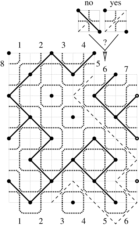
Figure 2: Computation of the partition function with twisted boundary conditions. Coloured edges (solid linestyle) connect the sites of the direct lattice (filled circles) so as to form clusters. The loops on the medial lattice (short boldface dashes) surround the clusters, and both cluster and loops are subject to periodic boundary conditions (indicated by open circles) across the strip of width $L=6$. A seam (long dashes) connecting sites of the dual lattice prevents the clusters and loops from wrapping around the cylinder. By adding a single vertex at a time the transfer matrix can be decomposed as a product of sparse matrices. Each multiplication by a single-vertex matrix corresponds graphically to augmenting the ‘jigsaw puzzle’ by one of the two ‘pieces’ shown in the top. In the situation at hand, one of these is forbidden by the twisted boundary conditions.

In Fig. 2 we show a configuration contributing to the partition function with twisted boundary conditions. As the square lattice is self-dual we shall take the clusters and loops to live on the direct lattice and its medial lattice respectively. The extended connectivity state of the $L$ (resp. $L+2$) dangling ends is the direct product of the $c_{L/2}$ possible connectivities mediated by the loops, and an integer specifying the position of the seam. The seam is a path inside the infinite dual cluster spanning the length of the cylinder, and after the addition of each vertex it must be updated according to the invariant that no loop closure take place across the seam.

Now consider the situation shown on Fig. 2 where we are about to add the fifth vertex of the top row. Since this is an even site the two possibilities for the loop configuration are those shown in the left part of Fig. 1. However, the first of these would lead to a forbidden loop closure, as witnessed by the fact that the seam is ‘trapped’ and cannot be updated. The corresponding entry in the transfer matrix is therefore zero, and only the graph realising the second possibility contributes.

Using the numbering of the $L$ (resp. $L+2$) dangling ends of an (in)complete row shown at the bottom (top) part of Fig. 2 it is easily seen that the seam position is always immediately to the right of an even end in every other row, and to the right of an odd end in the remaining rows. Therefore, in all cases the number of permissible seam positions is equal to half the number of dangling ends. The total number of extended $L$-point connectivity states is therefore

$$\frac{Lc_{L/2}}{2}=\frac{L!}{\left(\frac{L}{2}-1\right)!\left(\frac{L}{2}+1\right)!}\sim 2^{L}.$$ (4.42)

Taking into account that for a strip of width $L$ we need intermediate states of $(L+2)$-point connectivities, the size $N^{\rm alg4}_{N_{\rm mag}}$ of the transfer matrix for three coupled models with $N_{\rm mag}=1,2,3$ layers in the odd sector is as shown in Table 7. Note that for $N_{\rm mag}=1,2$ two of the layers are indistinguishable in the sense of Sec. 4.4.1, whilst for $N_{\rm mag}=3$ all three layers are indistinguishable.

$L$	$N_{\rm mag}=1$	$N_{\rm mag}=2$	$N_{\rm mag}=3$
2	12	20	20
4	225	600	680
6	5,880	22,344	30,856
8	189,630	930,510	1,565,620
10	6,952,176	41,451,696	83,112,744

Table 7: Number $N^{\tt alg4}_{N_{\rm mag}}(L)$ of basis states needed by alg4 to access the scaling exponents of the three-layered system that correspond to the insertion of a magnetisation operator in $N_{\rm mag}=1,2,3$ of the layers.

A very important remark pertains to the proper choice of the initial vector $|{\bf v}_{0}\rangle$ used for finding the largest eigenvalue, cfr. Eq. (4.3). Namely, when more than one layer is in the odd sector the seam positions on all layers must coincide at points $r_{1}$ and $r_{2}$. The reason why this is so can readily be illustrated for the case of two coupled models. With the initial vector (symbolically) chosen as $|{\bf v}_{0}\rangle=|1,1,1,\ldots\rangle\otimes|1,1,1,\ldots\rangle$ one would observe the asymptotic scaling of the correlator

$$\left\langle\sum_{r_{1},r_{1}^{\prime},r_{2},r_{2}^{\prime}}M_{a}^{(1)}(r_{1})M_{a}^{(2)}(r_{1}^{\prime})M_{a}^{(1)}(r_{2})M_{a}^{(2)}(r_{2}^{\prime})\right\rangle\sim\left\langle\sum_{r_{1},r_{2}}M_{a}(r_{1})M_{a}(r_{2})\right\rangle^{2},$$ (4.43)

where the summations run over the $L$ points at each extremity of the cylinder. At large distances $|r_{2}-r_{1}|\gg 1$ one would expect this to scale with the exponent $2x_{H}^{(1)}$, where $x_{H}^{(1)}$ is just the scaling dimension of the usual magnetisation operator. However, with $|{\bf v}_{0}\rangle=|1,0,0,\ldots\rangle\otimes|1,0,0,\ldots\rangle$ one would instead observe the scaling of

$$\left\langle\sum_{r_{1},r_{2}}M_{a}^{(1)}(r_{1})M_{a}^{(2)}(r_{1})M_{a}^{(1)}(r_{2})M_{a}^{(2)}(r_{2})\right\rangle,$$ (4.44)

and this should decay as $|r_{2}-r_{1}|^{-2x_{H}^{(2)}}$, where $x_{H}^{(2)}$ is the sought scaling dimension of the local operator $M_{a}^{(1)}(r)M_{a}^{(2)}(r)$. Indeed this is the simplest example of a multiscaling exponent as discussed by Ludwig [2] in the context of the random-bond Potts model ($N\to 0$).

The proper choice of $|{\bf v}_{0}\rangle$ is tantamount to anchoring all the seams at the point $r_{1}$. When applying Eq. (4.3) one should then theoretically project ${\bf T}^{|r_{2}-r_{1}|}|{\bf v}_{0}\rangle$ out on a state with a definite and identical seam position for all the layers before taking the norm. However, since we expect all the non-zero entries of the iterated vector to grow as $\exp\big{(}|r_{2}-r_{1}|\lambda(L)\big{)}$ this would just correspond to multiplying by a constant before taking the logarithm. Clearly such a constant would not contribute to the computed value of $\lambda(L)$, and so the projection can be omitted.

5 Numerical results

Using the transfer matrix algorithms just described we are able to find the effective values of the central charge and of the various thermal and magnetic scaling dimensions, all as functions of the coupling constant $a$, parametrising the position on the self-dual lines identified in Sec. 2. We are furthermore able to monitor the scale dependence of these quantities by changing the strip width $L$.

Let us briefly recapitulate the physical information that we hope to extract from these data. First, we should like to provide compelling evidence that, for $N>2$ coupled Potts models, a novel, non-trivial critical fixed point is located on the self-dual line, in the limit $a\to\infty$. We shall presently describe how such a conclusion may be attained from our numerical data. Second, we aim at fixing the values of the critical exponents at this fixed point. This is done by taking the limit $a\to\infty$ explicitly in the transfer matrices, in order to obtain high-precision data for rather large strip widths (up to $L=12$ for $N=3$). Extrapolating these data to the infinite system limit $L\to\infty$ we shall be able to identify the $a\to\infty$ fixed point with the one obtained from perturbative CFT in Sec. 3, and to associate the numerically obtained scaling dimensions with those of physical operators in the continuum limit. Third, we provide an independent check of the criticality of the fixed point under consideration. This is done by verifying the existence of scaling laws, using Monte Carlo simulations directly in the limit $a\to\infty$. As a by-product we extract values of the scaling dimensions that agree with the more precise estimates obtained from the transfer matrices. And fourth, we use our transfer matrices to inquire further into the structure of the (presently unknown) CFT governing the critical behaviour of the $a\to\infty$ model. To this end we take a closer look at the higher eigenvalues in the even sector. These data determine the scaling dimensions of less relevant operators in the Verma module, and they give crucial information of the operator content and descendence structure of the sought CFT. Finally, a comparison of the results obtained from algorithms alg3 and alg4 serves as a check of the modular invariance of the theory.

Although our main interest is $N=3$ coupled models we have also produced numerical results for the case of two coupled $q$-state Potts models, for several values of $q\in[2,4]$. For $q=2$ this is the Ashkin-Teller model. This model is critical on the entire half line $a\in[0,\infty]$, and it provides a useful check of our algorithms since the critical exponents are known exactly as a function of $a$ [37, 34]. For $q>2$, on the other hand, Vaysburd [19] has predicted a dynamical mass generation and thus a non-critical model. Since this prediction was made under several assumptions it is reassuring to see that our numerics confirms it. At the same time, our $N=2$ data provide a clear illustration of the difference between a first order phase transition scenario and a second order one.

5.1 Finding critical points from effective exponents

The key to the search for critical fixed points is, of course, Zamolodchikov’s $c$-theorem [8]. This theorem states that the effective central charge (the $c$-function) decreases along the RG flow and is stationary at its fixed points. In view of our definition (3.21) of the $c$-function, this is equivalent to the familiar statement that the $\beta$-function vanishes at a fixed point.

A local minimum (maximum) of the effective central charge thus corresponds to a (un)stable fixed point. When, as is the case here, the RG flow takes place in a multi-dimensional space of coupling constants one can also imagine the existence of saddle points, corresponding to a partially stable fixed point. But generically we expect the flow to take place along the self-dual line, and accordingly we can limit the search to this one-dimensional self-dual submanifold. This assumption is nicely corraborated by our numerical results. Indeed we find that in general any motion perpendicular to the self-dual line leads to a decrease of the central charge [see, e.g., Fig. 3.b and Fig. 10 below]. Hence, invoking duality, this line must serve as a mountain ridge for the central charge.

A notable exception to this scenario happens for the Ashkin-Teller model, where the self-dual half line $a\in[0,\infty]$ bifurcates into two mutually dual lines of critical points at $a=0$. However, this anomaly is very clearly signalled by the vanishing of the $c$-function of the other self-dual half line, $a\in[-\infty,0[$. We have not observed a similar situation for any other value of $q$, or of $N$.

Once a candidate for a fixed point has been identified the question arises whether it is critical or not. To address this point it is useful to examine the dependence of $c_{\rm eff}$ on the system size $L$. If a critical point is involved, the finite-size estimates $c_{\rm eff}(L)$ should converge very rapidly, with increasing $L$, to the true value of the central charge at this point. On the other hand, if the point is not critical a finite correlation length $\xi$ must be involved. As has been shown by Blöte and Nightingale [29] for the particular case of a first order phase transition, Eq. (4.4) for the finite-size scaling of the free energy must then replaced by

$$f_{0}(L)=f_{0}(\infty)-{\rm const.}\frac{{\rm e}^{-L/\xi}}{L^{2}}+\cdots.$$ (5.1)

This in turn implies that the effective central charge, i.e., the one measured assuming the scaling form (4.4), will vanish exponentially as a function of the strip width $L$. We shall soon see that our numerical data distinguish very easily between these two situations.

Complementary information about the location of possible fixed points is provided by the effective values of the thermal and magnetic scaling dimensions $x_{\rm eff}(L)$ along the self-dual line. In many situations a fixed point is signalled by the fact that the curves $x_{\rm eff}(L)$ and $x_{\rm eff}(L+1)$ intersect at some coupling $a(L)$. The finite-size estimates $a(L)$ then converge very rapidly towards the true value of the fixed-point coupling, as $L\to\infty$. Indeed, this is nothing but the well-known technique of phenomenological renormalisation [38]. Evidently a fixed point can also be characterised as a point of high symmetry. It is thus hardly surprising to see from our numerics, that in many cases local extrema of $x_{\rm eff}$ as a function of $a$ serve equally well to locate the position of the fixed point.

As was the case for the central charge, once a fixed point has been located its precise nature (critical or not) can be inferred by observing the size-dependence of $x_{\rm eff}(L)$. Since a finite correlation length implies an exponential, rather than a power law, decay of the various correlators, effective values of the scaling dimensions extracted from Eq. (4.5) will be observed to vanish exponentially with $L$, if $\xi<\infty$.

5.2 Two coupled models

5.2.1 Ashkin-Teller model

The case of two coupled Ising models is nothing but the well-known Ashkin-Teller model [39]. We shall nevertheless begin by investigating this case in order to demonstrate the method outlined above, and to see how we can reproduce known results.

Figure 3: Central charge for two coupled Ising models. (a) shows the effective central charge as a function of the parameter $a$. (b) corresponds to moving perpendicularly off the self-dual line.

As has been shown by Baxter [34] the isotropic Ashkin-Teller model can be mapped to a staggered eight-vertex model. This fact that this model is staggered seems to impede its solvability, but on the self-dual line given by Eq. (2.14), $a\in[-\infty,\infty]$, the eight-vertex model becomes homogeneous and hence soluble. For $a\geq 0$ the model is critical, with the following exact values of the critical exponents [37]:

$$c=1,\ \ \ \ x_{t}=\frac{1}{2-y},\ \ \ \ x_{H}^{(1)}=\frac{1}{8},\ \ \ \ x_{H}^{(2)}=\frac{1}{8-4y},$$ (5.2)

where

$$y=\frac{2}{\pi}{\rm arccos}\left({\rm e}^{-a}+\frac{1}{2}{\rm e}^{-2a}-\frac{1}{2}\right).$$ (5.3)

In Fig. 3.a we show the numerical values for the effective central charge, in the form of the three-point fits, cfr. Eq. (4.8). For every $a<0$ the central charge tends to zero in the large-system limit, indicating non-critical behaviour, and for $a\geq 0$ it approaches unity, in complete agreement with Eq. (5.2). The transfer matrix has also been diagonalised directly at $a=\infty$, again with the result $c\simeq 1$.

Figure 4: Thermal dimension $x_{t}$ and magnetic dimensions $x_{H}^{(1)}$, $x_{H}^{(2)}$ for two coupled Ising models.

Fig. 3.b depicts the behaviour of the central charge along a line perpendicular to the self-dual line at the point $a=2$. The value $a=2$ is chosen arbitrary, and we observe similar curves for other values of $a>0$. As we move into the non-self dual regime the central charge decreases, and the larger the strip width the faster the decrease. In the $L\to\infty$ limit we should have $c_{\rm eff}=0$ exactly. We can therefore conclude that the self-dual line indeed acts as a ridge of the central charge, thus confirming the hypothesis that the RG flow is along that line. We also observed that for $a<0$ the critical line bifurcates into two mutually dual Ising-like lines [34].

Next, in Fig. 4, we present measured values of the thermal scaling dimension, $x_{t}$, as well as the two magnetic ones, $x_{H}^{(1)}$ and $x_{H}^{(2)}$. As the $\beta$-function is exactly zero we can expect very accurate values, and as the comparison with the analytical results (5.2) shows this is indeed the case. The only exception is the point $a=0$, which corresponds to the 4-state Potts model. Due to the presence of a marginal operator there are strong logarithmic corrections [40], and the analytical results $x_{t}=1/2$ and $x_{H}^{(1)}=x_{H}^{(2)}=1/8$ are not accurately reproduced. Finally, by taking the explicit $a\to\infty$ limit in the transfer matrices we have verified the results $x_{t}=3/2$, $x_{H}^{(1)}=1/8$ and $x_{H}^{(2)}=3/8$.

5.2.2 Two coupled 3-state Potts models

Figure 5: Central charge for two coupled $3$-state Potts models (a) and two coupled $4$-state Potts models (b). The dots in (b) correspond to an interpolaton from the measurements made directly at $a=-\infty$ and $a=-5$. We also indicate by a cross a fit at $a=-\infty$ for strip widths $L$=10–14.

In the case $N=2$, $q=3$ there is an $a\leftrightarrow-a$ symmetry at the level of the free energy, as is reflected by the values of the effective central charge shown in Fig. 5. The origin of this symmetry becomes clear if one considers the possible local Boltzmann weigths $W(L_{ij},a)$ [cfr. Eq. (2.32)] associated with the interactions along edge $(ij)$. For two coupled $q$-state Potts models these are given by

$$W(0,a)=1,\ \ \ \ W(1,a)={\rm e}^{a},\ \ \ \ W(2,a)={\rm e}^{2a+b}=2{\rm e}^{a}+q-1.$$ (5.4)

In the transfer matrix, starting from an arbitrary state, the first weight will appear $(q-1)^{2}$ times, the second one $2(q-1)$ times, and the last one just once. Specialising now to $q=3$, we see that $W(0,a)$ and $W(1,a)$ have the same degeneracy, and that

$$W(0,-a)={\rm e}^{-a}W(1,a),\ \ \ \ W(1,-a)={\rm e}^{-a}W(0,a),\ \ \ \ W(2,-a)={\rm e}^{-a}W(2,a).$$ (5.5)

Thus we have established an exact symmetry for the specific free energy on the self dual line

$$f(-a,q=3)=f(a,q=3)-2a.$$ (5.6)

Returning to the central charge values shown in Fig. 5.a we see a local maximum at $a=\log(1+\sqrt{3})$, the fixed point corresponding to two decoupled 3-state Potts models. At this point the finite-size estimates converge very rapidly towards $c=2\times\frac{4}{5}$. The other trivial fixed point is located at $a=0$ and corresponds to a single 9-state Potts model. Here the estimates $c_{\rm eff}(L)$ decrease steadily with increasing strip width, as expected for a first order phase transition. Any model with a bare coupling $a_{0}>\log(1+\sqrt{3})$ renormalises towards the $a\to\infty$ fixed point, but this again corresponds to a first order transition [19] as witnessed by the steady decrease of the estimates for $c$.

5.2.3 Two coupled 4-state Potts models

$L$	$c(L,L+4)$	$x_{t}(L,L+2)$
4	2.251	1.032
6	2.231	0.856
8	2.203	0.808
10	2.175	0.762
12		0.720

Table 8: Effective exponents for two coupled 4-state Potts models at $a=-\infty$.

The effective central charge for two 4-state models can be inferred from Fig. 5.b, and apart from the disappearence of the $a\leftrightarrow-a$ symmetry conclusions are as in the case of two 3-state models. The range of $a$-values shown on the figure cannot entirely exclude the possibility of a novel fixed point at $a=-\infty$, but the data of Table 8, obtained by using alg4 directly at this point, tell us that if $a=-\infty$ indeed is a fixed point it must be unstable and non-critical.

5.2.4 The point $a=\infty$

As has already been stressed in Sec. 4 the topological algorithms alg3 and alg4 enable us to treat $q$, the number of Potts spin states, as a continuously varying parameter. We finish the discussion of the two-models case by presenting some results for the effective exponents for several fractional values of $q$, obtained directly in the $a\to\infty$ limit.

$q$	$c(4,8)$	$c(6,10)$	$c(8,12)$	$c(10,14)$	$c(12,16)$
2.00	0.988504	0.995838	0.998256	0.999142	0.999528
2.25	1.142687	1.149660	1.151260	1.151271	1.150843
2.50	1.263404	1.264818	1.260899	1.255641	1.250201
2.75	1.351006	1.338262	1.319944	1.300188	1.280109
3.00	1.406234	1.367834	1.322338	1.274092	1.224246
3.25	1.430583	1.353605	1.266530	1.174515	1.079463
3.50	1.426433	1.298639	1.157785	1.011642	0.864787
3.75	1.396976	1.208954	1.008126	0.807868
4.00	1.346005	1.092727	0.833815	0.590962

Table 9: Effective central charge for two coupled $q$-state Potts models at $a\to\infty$, obtained from alg4.

First, in Table 9 we display the central charge values. For $q=2$ these converge very nicely towards $c=1$, the exact Ashkin-Teller value (5.2). For higher $q$ the increasing spacing between succesive estimates signals non-critical behaviour, or in other words, the free energies are not well fitted by Eq. (4.4). It is convenient to have such data at one’s disposal, since they facilitate the distinguishing between first and second order phase transitions in the sequel. Evidently, for $q=2.25$ it not a priori easy to clearly point out the first order nature of the transition, since the correlation length is very large. However, it is interesting to notice that whilst for $q=2$ the estimates increase monotonically as a function of $L$, for all $q>2$ they eventually begin to decrease for large enough $L$.

$q$	$x_{t}(6,8)$	$x_{t}(8,10)$	$x_{t}(10,12)$	$x_{t}(12,14)$	$x_{t}(14,16)$
2.00	1.467238	1.475693	1.490527	1.495490	1.497566
2.25	1.745413	1.554317	1.588008	1.605994	1.618971
2.50	1.863461	1.768649	1.702778	1.739814	1.769780
2.75	1.780405	1.717780	1.672429	1.635165	1.603300
3.00	1.707436	1.630297	1.575072	1.532502	1.499100
3.25	1.648514	1.565197	1.510808	1.474971	1.452970
3.50	1.605054	1.524930	1.482309	1.464823	1.466231
3.75	1.576886	1.508815	1.487488	1.497813
4.00	1.562949	1.514505	1.521838	1.566459

Table 10: Effective values of the thermal scaling dimension for two coupled $q$-state Potts models at $a\to\infty$, obtained from alg4.

Table 10 provides the analogous estimates for the thermal scaling dimension. For $q=2$ they converge towards $x_{t}=3/2$, in accordance with Eq. (5.2). Otherwise their variation is not monotonic in $L$, presumably signalling the presence of a finite correlation length.

5.3 Three coupled models

We now turn to our primary interest, namely the case of $N=3$ coupled Potts models. The self-dual line here starts at the point where $b=-\infty$, that is $a\in[a_{\rm min},\infty]$ with

$$a_{\rm min}=\log\left(\frac{\sqrt{q}+1}{\sqrt{q}+2}\right).$$ (5.7)

Unlike the case of two models just discussed we shall find that the $a\to\infty$ limit corresponds to a critical fixed point for all values of $q\in[2,4]$. The determination of the associated critical exponents thus becomes of paramount interest, and we have dedicated considerable computational effort to this purpose. Let us discuss the various cases in turn.

5.3.1 Three coupled Ising models

Figure 6: Central charge for three coupled Ising models.

This is the three-colour Ashkin-Teller model. The effective central charge is displayed in Fig. 6.a. At the trivial fixed point at $a=0$ we find the usual dip in $c$, reflecting the first-order nature of the transition in the 8-state Potts model.

For all $a>0$ the central charge is approximately constant, $c\simeq 3/2$, and we have also verified this value in the limit $a\to\infty$. This situation is very reminiscent of that of the (standard) two-colour Ashkin-Teller model, and seems to allow for a situation where the entire half line $a>0$ consists of critical fixed points along which the critical exponents vary continuously. Whether this is indeed the case will be the subject of a separate publication [41].

Fig. 6.b presents a closer look at the antiferromagnetic region $a<0$. We find here a surprising candidate for an unstable critical fixed point at $a\simeq-0.22$ with a central charge of $c\simeq 1.5$. Further support for this suspicion is found in the maximum for the effective thermal exponent on Fig. 7.b, and in the crossing of the curves for the magnetic exponents on Fig. 8.b. More results along these lines will be published elsewhere [41].

Figure 7: Thermal exponent for three coupled Ising models.

The results for the thermal exponent on the half line $a>0$ are shown on Fig. 7.a. Everywhere the convergence seems to be very rapid, except at $a=0$ where we expect an extrapolated effective exponent of $x_{t}^{\rm eff}=0$ due to the first order transition. In the $a\to\infty$ limit we estimate $x_{t}=1.24\pm 0.01$; more detailed results are provided by Table 12 below.

Finally, in Fig. 8 we present results for the three different magnetic exponents, $x_{H}^{(1)}$, $x_{H}^{(2)}$ and $x_{H}^{(3)}$. The first exponent is constant, $x_{H}^{(1)}\simeq 1/8$ for $a>0$, as in the case of two coupled Ising models, whilst the other two depend on $a$. In the $a\to\infty$ limit we find $x_{H}^{(2)}\simeq 0.27$ and $x_{H}^{(3)}\simeq 0.46$ as witnessed by Tables 15 and 16.

Figure 8: Magnetic exponents for three coupled Ising models.

5.3.2 Three coupled 3-state Potts models

Until now, the models for which we have presented numerical data are believed to be somewhat atypical representatives for the general class of $N$ coupled $q$-state Potts models. On one hand, for $N=2$ coupled models the ${\cal O}(g^{2})$-term in the $\beta$-function (1.11) vanishes, and neighter perturbative RG nor numerics predict any non-trivial critical fixed points for $q\neq 2$. On the other, for $q=2$ the energy-energy coupling is exactly marginal, leading either to the Ashkin-Teller scenario with an entire line of critical fixed points along which the exponents vary continuously, or simply to a flow back towards the decoupled fixed point. For the case of $N=3$ coupled 3-state Potts models, which we consider now, the situation can thus be believed to be generic: Perturbation theory predicts a novel critical fixed point, Eq. (1.12), with unique critical exponents, and so does numerics, as we shall presently see.

Consider first the effective central charge along the self-dual line $a\in[a_{\rm min},\infty]$, where $a_{\rm min}=\log\left(\frac{\sqrt{3}+1}{\sqrt{3}+2}\right)$. On Fig. 9.a we recognise the familiar structure of a local minimum and a local maximum, signaling the usual two trivial fixed points. However, for larger values of $a$ a novel feature emerges, as witnessed by Fig. 9.b. The central charge is here a very slightly decreasing function of $a$, indicating a flow towards the fixed point at $a=\infty$. Furthermore, the finite-size dependence of the estimates leads us to the conclusion that this point is now critical.

Figure 9: Central charge for three coupled 3-state Potts models. The dots designate an interpolation from $a=4.5$ to $a=+\infty$.

The more accurate data of Table 11 corroborate this scenario. First, we see that the finite-size estimates converge very rapidly to the value

$$c=2.377\pm 0.003,$$ (5.8)

in very good agreement with the perturbative prediction $c_{\rm FP}=2.3808+{\cal O}(\epsilon^{5})$ from Eq. (3.23). Second, the convergence of the estimates in Table 11 is now from below, convincingly excluding the possibility that $c_{\rm eff}$ could eventually tend to zero, as would be the case for a non-critical fixed point. Third, the numerical value for $c$ is comfortably away from that of the decoupled fixed point, $c_{\rm pure}=3\times\frac{4}{5}=2.4$.

Figure 10: Central charge for three coupled 3-state Potts models when moving perpendicularly off the self-dual line.

Figure 11: Thermal exponent for $x_{t}$ for three coupled $q$-state Potts models with $q=3$ and $q=4$ respectively.

In Fig. 10 we show the behaviour of the central charge along a line perpendicular to the self-dual line at the point $a=1.19217$. Once again, this value of $a$ was chosen arbitrarily; similar curves are observed for other values of $a>0$.

Plots of the effective thermal and magnetic exponents are shown in Figs. 11.a and 12.a respectively. More accurate values obtained directly at the $a=\infty$ critical point are given in Table 12–16.

Figure 12: Magnetic exponents $x_{H}^{(1)}$, $x_{H}^{(2)}$ and $x_{H}^{(3)}$ for three coupled $q$-state Potts models with $q=3$ and $q=4$ respectively.

5.3.3 Three coupled 4-state Potts models

The situation for three coupled Potts models is very similar to the case of $q=3$ treated above. The plots of the effective central charge given in Fig. 13 again give us strong reasons to believe that the $a\to\infty$ limit represents the non-trivial critical fixed point predicted by perturbation theory. Also the effective thermal and magnetic exponents of Figs. 11.b and 12.b respectively exhibit a structure similar to the $q=3$ case, but the critical exponents at $a\to\infty$ are of course distinct.

Figure 13: Central charge for three coupled $4$-state Potts models.

5.3.4 The $a\to\infty$ limit for general $q\in[2,4]$

After having numerically identified the non-trivial critical fixed point for three coupled models, that was predicted by the perturbative RG, we would like to accurately determine the associated critical exponents as a function of $q$. This is done by diagonalising the transfer matrix directly at $a=\infty$, using alg4.

In Table 11 we show finite-size estimates of the central charge, obtained from three-point fits of the form (4.8). For all $q\in[2,4]$ these estimates seems to converge as $L\to\infty$. Of course, an explicit extrapolation to the infinite system limit from just three data points would easily turn out to be rather subjective. It should however be noted that the convergence is in most cases monotonic, and the last estimate therefore provides a quite accurate upper or lower bound for the extrapolated quantity.

$q$	$c(4,8)$	$c(6,10)$	$c(8,12)$
2.00	1.489114	1.497443	1.500008
2.25	1.747538	1.757162	1.760185
2.50	1.976384	1.986719	1.989905
2.75	2.179933	2.190166	2.193005
3.00	2.361502	2.370594	2.372345
3.25	2.523740	2.530453	2.530147
3.50	2.668818	2.671752	2.668217
3.75	2.798557	2.796195	2.788092
4.00	2.914511	2.905265	2.891139

Table 11: Results for the central charge of three coupled models at $a=\infty$ and for varying values of $q$.

The results for $c$ are in very good agreement with the perturbative RG in the range $q\in[2,3]$. For larger values of $q$ the perturbation theory is expected to break down, and so the numerical values are likely to be more reliable.

$q$	$x_{t}(6,8)$	$x_{t}(8,10)$	$x_{t}(10,12)$
2.00	1.257900	1.248706	1.242186
2.25	1.263919	1.255942	1.250623
2.50	1.268895	1.262901	1.259341
2.75	1.272294	1.268558	1.266905
3.00	1.273618	1.271938	1.271901
3.25	1.272423	1.272143	1.272966
3.50	1.286448	1.268344	1.268400
3.75	1.261129	1.260138	1.258753
4.00	1.250663	1.247052	1.242082

Table 12: Results for the thermal scaling dimension of three coupled models at $a=\infty$ using alg4.

The corresponding values of the thermal scaling dimension are given in Table 12. In this case the comparison with the perturbative results is more tricky. We recall that $x_{t}$ is obtained by fitting the first gap in the even sector of the transfer matrix to Eq. (4.9). This is expected to correspond to the scaling dimension of the most relevant symmetric energy operator, $\varepsilon_{1}+\varepsilon_{2}+\varepsilon_{3}$. However, $\Delta_{\varepsilon_{1}+\varepsilon_{2}+\varepsilon_{3}}$ has only been determined to order ${\cal O}(\epsilon^{3})$ [see Eq. (3.11)], and so the discrepancy between the values of Table 12 and of Table 1 for large $q$ should hardly come as a surprise. On the other hand, for $q$ slightly larger than two numerics is supposed to be hampered by large logarithmic corrections due to the near-marginality of the energy operator [40]. In this range we thus expect the perturbative results to be the more reliable.

$q$	$c(3,5)$	$c(4,6)$	$x_{t}(4,5)$	$x_{t}(5,6)$
2.00	1.5040	1.4906	1.2692	1.2600
2.25	1.7653	1.7490	1.2798	1.2691
2.50	1.9965	1.9775	1.2890	1.2774
2.75	2.2022	2.1801	1.2964	1.2842
3.00	2.3856	2.3601	1.3018	1.2890
3.25	2.5495	2.5198	1.3051	1.2913
3.50	2.6962	2.6615	1.3062	1.2907
3.75	2.8274	2.7869	1.3049	1.2868
4.00	2.9449	2.8975	1.3011	1.2796

Table 13: Results for three models at $a\to\infty$ using alg3.

In Table 13 we show some more results for $c$ and $x_{t}$, but this time obtained from alg3. The usefulness of these data is twofold. First, they clearly demonstrate the superiority of alg4 as regards the accuracy and the convergence properties (monotonicity) of the finite-size estimates. Second, the agreement with Table 11–12 serves as a check of the modular invariance of the $a=\infty$ critical point, as explained in Sec. 4.7.

$q$	$x^{(1)}_{H}(4,6)$	$x^{(1)}_{H}(6,8)$	$x^{(1)}_{H}(8,10)$
2.00	0.124815	0.125054	0.125112
2.25	0.127712	0.127847	0.127851
2.50	0.129955	0.129915	0.129810
2.75	0.131635	0.131334	0.131050
3.00	0.132825	0.132170	0.131623
3.25	0.133588	0.132480	0.131577
3.50	0.133977	0.132318	0.130962
3.75	0.134040	0.131734	0.129831
4.00	0.133816	0.130778	0.128237

Table 14: $x_{H}^{(1)}$ for three coupled Potts models at $a=\infty$.

We now turn our attention to the magnetic exponents $x_{H}^{(N_{\rm mag})}$ obtained by imposing twisted boundary conditions on $N_{\rm mag}=1,2$ or 3 of the $N=3$ coupled Potts models. The numerical results are presented in Table 14–16. Comparing with the analytic results of Table 1–2 we find, as expected, that these scaling exponents must be those of the first three moments of the magnetisation. Excluding the case of $q=2$ where the remarks made above hold true, we find a very good agreement between $x_{H}^{(1)}$ and $\Delta_{\sigma_{1}}$, and between $x_{H}^{(2)}$ and $\Delta_{\sigma_{1}\sigma_{2}}$ in the range $q\leq 3$. For larger $q$ the perturbative RG breaks down with a vengeance, as witnessed by its predictions of negative scaling dimension.

Finally, the agreement between $x_{H}^{(3)}$ and $\Delta_{\sigma_{1}\sigma_{2}\sigma_{3}}$, especially in the range $2.5<q<3.5$, is quite striking, and is the first validation of the second order perturbative computation proposed previously by one of us [20].

$q$	$x^{(2)}_{H}(4,6)$	$x^{(2)}_{H}(6,8)$	$x^{(2)}_{H}(8,10)$
2.00	0.277424	0.276866
2.25	0.287411	0.287143	0.286780
2.50	0.296026	0.295985	0.295839
2.75	0.303408	0.303470	0.303445
3.00	0.309671	0.309661	0.309600
3.25	0.314915	0.314615	0.314310
3.50	0.319226	0.318393	0.317599
3.75	0.322685	0.321061	0.319512
4.00	0.325367	0.322693	0.320119

Table 15: $x_{H}^{(2)}$ for three coupled Potts models at $a=\infty$.

$q$	$x^{(3)}_{H}(4,6)$	$x^{(3)}_{H}(6,8)$	$x^{(3)}_{H}(8,10)$
2.00	0.475424	0.471563
2.25	0.503049	0.500930
2.50	0.529688	0.529874
2.75	0.555511	0.558541
3.00	0.580638	0.587025	0.592223
3.25	0.605162	0.615388
3.50	0.629150	0.643668
3.75	0.652656	0.671885
4.00	0.675719	0.700047	0.721371

Table 16: $x_{H}^{(3)}$ for three coupled Potts models at $a=\infty$.

5.3.5 Higher exponents in the even sector for $N=3$, $q=3$

In an attempt to numerically identify more of the operators predicted by perturbation theory, we have looked at the scaling dimensions extracted from the finite-size scaling of higher gaps in the even sector of the transfer matrix. These computations are extremely time-consuming, since, in order to study the first $k$ gaps, we need to iterate and orthogonalise $k+1$ vectors, cfr. Eq. (4.3). We have therefore focused exclusively on the case of three coupled 3-state Potts models.

The primary operators we expect to find in the even sector must all be energetic, since the $Z_{q}$ symmetry associated with the permutation of the Potts spin labels has been factored out. Furthermore, since alg4 by construction treats all three layers symmetrically, we only expect to find such operators that are symmetric under any permutation of the layer indices. According to Sec. 3 the permissible operators are thus

$$I,\ \ \ \ \varepsilon_{1}+\varepsilon_{2}+\varepsilon_{3},\ \ \ \ \varepsilon_{1}\varepsilon_{2}+\varepsilon_{2}\varepsilon_{3}+\varepsilon_{3}\varepsilon_{1},\ \ \ \ \varepsilon_{1}\varepsilon_{2}\varepsilon_{3}.$$ (5.9)

If the (presently unknown) conformal field theory of the system can be assumed to have the usual structure [42] we can, in addition to these primaries, in general expect to find descendent operators with their appropriate degeneracies, reflecting the null vector structure of the Verma module. The identity operator $I$ can be thought of as the primary corresponding to the zeroth gap, thus having scaling dimension $\Delta_{I}=0$ by definition.

Gap	$x(4)$	$x(6)$	$x(8)$	$x(10)$	$x(12)$	Extrapolation	Operator
1	1.694	1.471	1.385	1.344	1.322	1.27	$\varepsilon_{1}+\varepsilon_{2}+\varepsilon_{3}$
2	2.603	2.380	2.272	2.219	2.148	$\approx 2.0$	$T=L_{-1}I$
3	2.922	2.775	2.398	2.225	2.148	$\approx 2.0$	$\overline{T}=\overline{L}_{-1}I$
4	—	3.104	2.398	2.225	2.174	$\approx 2.1$	$\varepsilon_{1}\varepsilon_{2}+\varepsilon_{2}\varepsilon_{3}+\varepsilon_{3}\varepsilon_{1}$
5	—	3.104	2.685	2.633	2.599	$\approx 2.3$	$L_{-1}(\varepsilon_{1}+\varepsilon_{2}+\varepsilon_{3})$
6	—	3.626	3.279	2.785	2.598	$\approx 2.3$	$\overline{L}_{-1}(\varepsilon_{1}+\varepsilon_{2}+\varepsilon_{3})$
7	—	3.991	3.279	2.785	2.598	$\approx 2.4$	$\varepsilon_{1}\varepsilon_{2}\varepsilon_{3}$
8	—	3.991	3.289	3.146	3.066	$\approx 3.0$	$T^{\prime}=L_{-3}I$

Table 17: Scaling dimensions extracted from the higher gaps in the even sector as well as their identification with physical operators.

In Table 17 we show the results for the first eight gaps, obtained by employing alg4. Since we do not wish to make any a priori assumptions on the existence of the stress tensor we report only the unadorned one-point fits (4.5), for strip widths up to $L=12$. For $L=4$ we were only able to iterate four orthogonal vectors, and consequently there are some empty entries in the table.

The extrapolation to the $L\to\infty$ limit becomes increasingly important for the higher gaps, but unfortunately also increasingly difficult, since the convergence is slower and there are fewer data points. The reported values of the extrapolated scaling dimensions are therefore only indicative.

Let us recall from Sec. 3 that perturbation theory predicts

$$\Delta_{\varepsilon_{1}+\varepsilon_{2}+\varepsilon_{3}}\simeq 1.44,\ \ \ \ \Delta_{\varepsilon_{1}\varepsilon_{2}+\varepsilon_{2}\varepsilon_{3}+\varepsilon_{3}\varepsilon_{1}}\simeq 2.08,\ \ \ \ \Delta_{\varepsilon_{1}\varepsilon_{2}\varepsilon_{3}}\simeq 2.28.$$ (5.10)

These values cannot be believed to be very precise, since at $q=3$ we expect the perturbative expansion to be at the verge of breaking down. Nevertheless, they are supposed to be of the right order of magnitude, and we thus venture to make the identification shown in Table 17.

Note that for $L\geq 8$ the 3rd and the 4th gap, and also the 6th and the 7th, are exactly degenerate with full 16-digit machine precision. One would therefore expect them to be connected by a simple symmetry, as reflected by our conjectured identification. However, for $L=12$ a crossover takes place so that henceforth it is the second and the third gap that are degenerate rather than the third and the fourth. This could have been anticipated by noticing that for $L<12$ gaps 2–4 have quite different finite-size dependence. A similar crossover is expected to take place amongst gaps 5–7 for $L=14$. Accordingly our operator identifications pertain to the expected arrangement of the gaps in the $L\to\infty$ limit.

Apart from the primaries (5.9) we are able to identify the holomorphic and antiholomorphic components of the stress tensor, both with scaling dimension two. This provides further evidence for the criticality of the system, and is completely independent of the methods used this far. In addition we observe the level-one descendents of the operator $\varepsilon_{1}+\varepsilon_{2}+\varepsilon_{3}$ with the expected scaling dimension.

Unfortunately we have not been able to iterate enough vectors to see descendents at level two. This is a pity, since the degeneracy of these scaling dimensions would enable us to make predictions about the null vector structure of the Verma module.

5.3.6 Monte Carlo Results

Showing the existence of scaling operators, whose correlators obey scaling laws, would confirm that the $a\to\infty$ limit point on the self-dual line for three coupled models can be identified with a second order phase transition. To do so, we performed Monte Carlo (MC) simulations with the simplified Boltzmann weights (2.36) pertaining to this point. A direct measure of correlators for the physically significant operators (i.e. those which are diagonal in the perturbation scheme) clearly shows that the model is indeed critical, exhibiting scaling laws with associated exponents sufficiently close to those obtained either by perturbative CFT or transfer matrix techniques. Since the critical exponents can be measured with much more accuracy using transfer matrices techniques, MC was used solely to establish the criticality of the fixed point model.

We chose to measure explicitly the correlation functions for the spin and energy operators. Whilst the definition of energy correlators is straightforward, the $Z_{q}$ symmetry of spin variables has to be taken into account, and one should rather consider the operators

$$\Sigma_{i}\equiv\sigma_{i}-\overline{\sigma_{i}}\qquad\mbox{mod }q,$$ (5.11)

where $\overline{\sigma_{i}}$ is the instantaneous average value of the spin $\sigma$ on lattice $i$. The physically meaningful operators, for which we computed correlators, are thus the following:

$$\varepsilon_{S} \equiv \varepsilon_{1}+\varepsilon_{2}+\varepsilon_{3}$$ (5.12)

$$\varepsilon_{A} \equiv \varepsilon_{1}-\varepsilon_{2}$$ (5.13)

$$\Sigma_{S} \equiv \Sigma_{1}+\Sigma_{2}+\Sigma_{3}$$ (5.14)

$$\Sigma_{A} \equiv \Sigma_{1}-\Sigma_{2}.$$ (5.15)

These operators have well-behaved distributions and are the ones obeying scaling laws. We performed simulations on a $160\times 160$ lattice with periodic boundary conditions in both directions. Sixteen runs of 10,000 sweeps each were made, with a preliminary thermalisation stage of 500 times the autocorrelation time (which is around 25 updates for our lattice size). We also checked that the values of critical exponents were rather close to those predicted using this lattice size. A larger lattice would evidently provide a better description of critical behaviour, but computation time grows rapidly with the number of spins and, as we said, a precise measurement of critical exponents is not what was sought here.

Simulations were performed using a modified version of the Wolff one-cluster algorithm [43]. Let us consider the model given by Eq. (2.16), which we recall:

$${\cal H}_{ij} = a\,(\delta_{\sigma_{i},\sigma_{j}}+\delta_{\tau_{i},\tau_{j}}+\delta_{\eta_{i},\eta_{j}})+b\,(\delta_{\sigma_{i},\sigma_{j}}\delta_{\tau_{i},\tau_{j}}+\delta_{\sigma_{i},\sigma_{j}}\delta_{\eta_{i},\eta_{j}}+\delta_{\tau_{i},\tau_{j}}\delta_{\eta_{i},\eta_{j}})$$ (5.16)

$$+ c\,\,\delta_{\sigma_{i},\sigma_{j}}\delta_{\tau_{i},\tau_{j}}\delta_{\eta_{i},\eta_{j}}.$$

We first choose randomly one of the three models, say the one with the indices $\sigma$ (the model is invariant under permutation of any pair of layers). Then, we consider the model defined by

$${\cal H}_{ij} = (a+b\,(\delta_{\tau_{i},\tau_{j}}+\delta_{\eta_{i},\eta_{j}})+c\,\,\delta_{\tau_{i},\tau_{j}}\delta_{\eta_{i},\eta_{j}})\delta_{\sigma_{i},\sigma_{j}}+{\rm const.}$$ (5.17)

$$= a^{\prime}\delta_{\sigma_{i},\sigma_{j}}+{\rm const.}$$ (5.18)

Next we update the lattice with the usual Wolff algorithm but with the local $a^{\prime}=a+b\,(\delta_{\tau_{i},\tau_{j}}+\delta_{\eta_{i},\eta_{j}})+c\,\,\delta_{\tau_{i},\tau_{j}}\delta_{\eta_{i},\eta_{j}}$. Repeated three times, this operation defines one update of the system.

The measurement procedure is quite straightforward: For a given operator ${\cal O}$, all correlation functions $G(|x-y|)\equiv\langle{\cal O}(x){\cal O}(y)\rangle$, which are manifestly translationally invariant due to the choice of boundary conditions, are computed for $0<|x-y|<80$. Compiling results, one finds that the region where scaling laws exist is limited to $|x-y|<20$ for all operators, except for the symmetric energy, whose scaling law behaviour is observed only for $|x-y|<8$, this being due to the fact that the critical exponent for this operator is much larger than for the others. This is quite deceiving, but not unexpected. It is clear that for critical correlations to have some sense, they must be between points $x$ and $y$ such that $|x-y|\ll L$. This, combined with the fact that our statistics were rather low, explains why we had to restrict our attention to such narrow regions. Doing so, one observes nice scaling properties with associated exponents close to the ones computed by other analytical and numerical methods. Figures 14 and 15 present the Log-Log plot of correlation functions along with statistical error bars. Linear fits of these graphs give $2\Delta_{\cal O}$, and thus leads to the following values for the critical exponents:

$$\Delta_{\varepsilon_{S}} \equiv 1.27\pm 0.13$$ (5.19)

$$\Delta_{\varepsilon_{A}} \equiv 0.63\pm 0.04$$ (5.20)

$$\Delta_{\Sigma_{S}} \equiv 0.13\pm 0.03$$ (5.21)

$$\Delta_{\Sigma_{A}} \equiv 0.10\pm 0.03.$$ (5.22)

Altough not precise, the MC data clearly establish the existence of scaling operators. This confirms that the model under study is critical.

Figure 14: (a) Monte Carlo results for $\log\langle\varepsilon_{A}(x)\varepsilon_{A}(y)\rangle$ as a function of $\log|x-y|$. (b) $\log\langle\varepsilon_{S}(x)\varepsilon_{S}(y)\rangle$ as a function of $\log|x-y|$.

Figure 15: (a) Monte Carlo results for $\log\langle\Sigma_{A}(x)\Sigma_{A}(y)\rangle$ as a function of $\log|x-y|$. (b) $\log\langle\Sigma_{S}(x)\Sigma_{S}(y)\rangle$ as a function of $\log|x-y|$.

6 Concluding remarks

Besides the long-reaching goal of describing exactly disordered systems, the extensive study presented here is, we hope, interesting in many aspects. First, it introduces a new variant of the Potts model transfer matrix method which proves to be the most accurate and efficient up to now. Second, we have identified non-trivial fixed points both numerically and analytically and have presented evidence that these two types of fixed points are indeed the same and correspond to non-trivial critical models. The universality classes of these critical models are new, and several critical exponents were computed for the first time.

The next step in our long-term project is to solve the critical model, which was proven to be the end-point of the self-dual line. At this point, as we have shown, the Hamiltonian simplifies greatly, and it might be possible to map the system to a loop model, whose continuum limit is a Liouville field theory [36]. We believe that the results presented here will be of the outmost importance when searching for such a loop formulation.

Acknowledgments

We would like to thank P. Pujol for valuable discussions. M.-A.L. acknowledges financial support from NSERC Canada.

References

- [1] Vik. S. Dotsenko and Vl. S. Dotsenko, Sov. Phys. JETP Lett. 33, 37 (1981); J. Phys. A 17, L301 (1984).
- [2] A. W. W. Ludwig, Nucl. Phys. B 285, 97 (1987); Nucl. Phys. B 330, 639 (1990).
- [3] Vl. S. Dotsenko, M. Picco and P. Pujol, Phys. Lett. B 347, 113 (1995), hep-th/9405003; Nucl. Phys. B 455, 701 (1995), hep-th/9501017.
- [4] S. Chen, A. M. Ferrenberg and D. P. Landau, Phys. Rev. Lett. 69, 1213 (1992); Phys. Rev. E 52, 1377 (1995).
- [5] M. Picco, Phys. Rev. Lett. 79, 2998 (1997), cond-mat/9704221; cond-mat/9802092.
- [6] J. Cardy and J. L. Jacobsen, Phys. Rev. Lett. 79, 4063 (1997), cond-mat/9705038; J. L. Jacobsen and J. Cardy, Nucl. Phys. B 515 [FS], 701 (1998), cond-mat/9711279.
- [7] C. Chatelain and B. Berche, Phys. Rev. Lett. 80, 1670 (1998), cond-mat/9801028; Phys. Rev. E 58, R6899 (1988), cond-mat/9810270.
- [8] A. B. Zamolodchikov, Pis’ma Zh. Eksp. Teor. Fiz. 43, 565 (1986) [English translation in JETP Lett. 43 (1986) 730]; Sov. J. Nucl. Phys. 46 (1987) 1090.
- [9] R. J. Baxter, J. Phys. C 6, L445 (1973).
- [10] F.Y. Wu and Y.K. Wang, J. Math. Phys. 17, 439 (1976).
- [11] E. Domany and E. K. Riedel, Phys. Rev. B 19, 5817 (1979).
- [12] J. L. Cardy, J. Phys. A 26, 1897 (1996), cond-mat/9511112.
- [13] P. Pujol, Europhys. Lett. 35, 283 (1996), cond-mat/9602116.
- [14] P. Simon, Nucl. Phys. B 515, 624 (1998), cond-mat/9710024.
- [15] M.-A. Lewis and P. Simon, Phys. Lett. B 435, 159 (1998), cond-mat/9805026.
- [16] R. J. Baxter, Phys. Rev. Lett. 26, 832 (1971); L. P. Kadanoff and F. J. Wegner, Phys. Rev. B 4, 3989 (1971); F. Y. Wu, Phys. Rev. B 4, 3212 (1971).
- [17] E. Fradkin, Phys. Rev. Lett. 53, 1967 (1984).
- [18] R. Shankar, Phys. Rev. Lett. 55, 453 (1985).
- [19] I. Vaysburd, Nucl. Phys. B 446, 387 (1995).
- [20] M.-A. Lewis, Europhys. Lett. 43(2), 189 (1998), cond-mat/9710312.
- [21] Vik. S. Dotsenko, Vl. S. Dotsenko and M. Picco, Nucl. Phys. B 520, 633 (1998), hep-th/9709136.
- [22] H. W. J. Blöte and M. P. Nightingale, Physica A 112, 405 (1982).
- [23] H. Furstenberg, Trans. Am. Math. Soc. 108, 377 (1963).
- [24] G. Benettin, L. Galgani, A. Giorgilli and J.-M. Strelcyn, Meccanica 15, 9 (1980).
- [25] M. P. Nightingale, in Finite-size scaling and numerical simulations of statistical systems, edited by V. Privman (World Scientific, Singapore, 1990).
- [26] H. Blöte, J. L. Cardy and M. P. Nightingale, Phys. Rev. Lett. 56, 742 (1986).
- [27] I. Affleck, Phys. Rev. Lett. 56, 746 (1986).
- [28] J. L. Cardy, J. Phys. A 16, L355 (1983).
- [29] H. Blöte and M. P. Nightingale, Physica A 112, 405 (1982).
- [30] J. L. Cardy in C. Domb and J. L. Lebowitz (eds.), Phase transitions and critical phenomena, vol. 11 (Academic Press, London, 1987).
- [31] F. Y. Wu and H. Y. Huang, Phys. Rev. Lett. 79, 4954 (1997).
- [32] I. S. Gradshteyn and I. M. Ryzhik, Table of Integrals, Series and Products, 4. ed. (Academic Press, New York, 1965).
- [33] P. W. Kasteleyn, Physica 29, 1329 (1963).
- [34] R. J. Baxter, Exactly solved models in statistical mechanics (Academic Press, New York, 1982).
- [35] H. W. J. Blöte and B. Nienhuis, J. Phys. A 22, 1415 (1989).
- [36] J. L. Jacobsen and J. Kondev, Nucl. Phys. B 532 [FS], 635 (1998), cond-mat/9804048.
- [37] L. P. Kadanoff, Phys. Rev. Lett. 39, 903 (1977); Ann. Phys. (N.Y.) 120, 39 (1979); L. P. Kadanoff and A. C. Brown, Ann. Phys. (N.Y.) 121, 318 (1979).
- [38] M. P. Nightingale, Physica A 83, 561 (1976).
- [39] J. Ashkin and E. Teller, Phys. Rev. 64, 178 (1943).
- [40] J. L. Cardy, J. Phys. A 19, L1093 (1986).
- [41] Vl. Dotsenko, J. L. Jacobsen, M.-A. Lewis and M. Picco, in preparation.
- [42] A. A. Belavin, A. M. Polyakov and A. B. Zamolodchikov, Nucl. Phys. B 241, 333 (1984).
- [43] U. Wolff, Phys. Rev. Lett. 60, 1461 (1988).