Critical behavior of a traffic flow model

Abstract

The Nagel-Schreckenberg traffic flow model shows a transition from a free flow regime to a jammed regime for increasing car density. The measurement of the dynamical structure factor offers the chance to observe the evolution of jams without the necessity to define a car to be jammed or not. Above the jamming transition the dynamical structure factor exhibits for a given $k$-value two maxima corresponding to the separation of the system into the free flow phase and jammed phase. We obtain from a finite-size scaling analysis of the smallest jam mode that approaching the transition long range correlations of the jams occur.

]

I Introduction

Real traffic displays with increasing car density a transition from free flow traffic to congested traffic. This break down of free flow traffic is accompanied by the occurrence of traffic jams which are not attributable to any external cause but only to distance fluctuations between following vehicles within very dense and unstable traffic (see for instance [4]). These traffic jams find expression in shock waves, i.e., in backward moving density fluctuations. This property of jams was already found during the 60’s in traffic observations [5]. Beyond this early experimental investigations recently performed measurements of real highway traffic leads to the conjecture that jams are characterized by several independent parameters, e.g., the jam velocity, mean flux, etc. [6].

Since the seminal work of Lighthill and Whitham in the middle of the 50’s [7] many attempts have been made to construct more and more sophisticated models which incorporate various phenomena occurring in real traffic (for an overview see [8, 9]). Few years ago Nagel and Schreckenberg [10] introduced a cellular automata model, which simulates single-lane one-way traffic, and which is able to reproduce the main features of traffic flow, backward moving shock waves and the so-called fundamental diagram (see [11] and references therein). Investigations of the Nagel-Schreckenberg traffic flow model show that crossing a critical point a transition takes place from a homogeneous regime (free flow phase) to an inhomogeneous regime which is characterized by a coexistence of the free flow phase and the jammed phase [12, 13]. Thereby, the free flow phase is characterized by a low local density and the jammed phase by a high local density, respectively. Due to the particle conservation of the model the transition is realized by the system separating into a low density region and a high density region [12]. Despite several attempts it is still an open question wether the transition can be described as a critical phenomenon (see for instance [12, 14, 15, 16, 17]).

An attempt to investigate the occurrence of jam was made by Vilar and Souza [14] who introduced an order parameter which equals the number of standing cars. Without noise this quantity vanishes continuously below the transition. But including noise the amount of standing cars is finite for any nonzero density, i.e., the average number of standing cars does not vanish below the critical density. The crucial point is that below the transition a particle may stop due to the noisy slowing down rule of the dynamics, but this behavior does not coincide with backward moving density fluctuations and algebraic decaying correlation functions which would indicate a critical behavior of the system. At present, a convincing definition of an order parameter, which tends below the critical density to zero, is not known. Again, it is even not clear wether the Nagel-Schreckenberg traffic flow model displays criticality at all.

We use the dynamical structure factor both to make predictions about the properties of the different phases observed in the Nagel-Schreckenberg model and to investigate the question wether the occurrence of jam can be described as a phase transition or not. The dynamical structure factor which is closely related to the correlation function is an appropriate tool to do this because it naturally distinguishes between the two phases characterized by positive and negative velocities (free traffic flow and backward moving shock waves). Thus the advantage of our method of analyses is that the properties of both phases can be examined without the necessity to define a car to be jammed or not. The paper is organized as follows: In Sec. II we briefly describe our analysis of the dynamical structure factor and recall the main results which were published recently [18]. In Sec. III we extend this method of analysis to the so-called velocity-particle space and address the question whether the transition from the free flow regime to the phase coexisting regime (where the system separates into the jammed and free flow phase) can be considered as a phase transition. Basing on the dynamical structure factor, our results suggest that a continuous phase transition takes place.

II Model and Simulations

The Nagel-Schreckenberg traffic flow model [10] is based on a one-dimensional cellular automaton of linear size $L$ and $N$ particles. Integer values describing the position $r_{n}\in\{1,2,...,L\}$, the velocity $v_{n}\in\{0,1,...,v_{\rm max}\}$ and the gap $g_{n}$ to the forward neighbor are associated with each particle. For each particle, the following update steps representing the acceleration, the slowing down, the noise, and the motion of the particles are done in parallel: (1) if $v_{n}<g_{n}$ the velocity is increased with respect to the maximal velocity, $v_{n}\to\mbox{Min}\{v_{n}+1,v_{\rm max}\}$, (2) to avoid crashes the velocity is decreased by $v_{n}\to g_{n}$ if $v_{n}>g_{n}$, (3) if $v_{n}>0$ the velocity is decreased by $v_{n}\to v_{n}-1$ with probability $P\/$ in order to allow fluctuations, and finally (4) the motion of the cars is given by $r_{n}\to r_{n}+v_{n}$. Thus the behavior of the model is determined by three parameters, the maximal velocity $v_{\rm max}$, the noise parameter $P$ and the global density of cars $\rho=N/L$, where $N$ denotes the total number of cars and $L$ the system size, which is chosen to be $L=32768$ throughout the whole paper.

Our analyses is based on the dynamical structure factor whose definition is as follows: Consider the occupation function

$$\eta_{r,t}\;=\;\left\{\begin{array}[]{l}1\hskip 14.22636pt\mbox{if cell $r$ is occupied at time $t$}\\ 0\hskip 14.22636pt\mbox{otherwise}\,.\end{array}\right.$$ (1)

The evolution of $\eta_{r,t}$ leads directly to the space-time diagram where the propagation of the particles can be visualized (see for instance Fig. 2 in [19]). The dynamical structure factor $S(k,\omega)$ is then given by

$$S(k,\omega)\;=\;\frac{1}{l\,T}\;\left\langle\left|\;{\displaystyle\sum_{r,t}}\,\eta_{r,t}\;e^{i(kr-\omega t)}\right|^{2}\right\rangle\,,$$ (2)

where the Fourier transform is taken over a finite rectangle of the space-time diagram of size $l\times T$, i.e., $r$ and $t$ are integers ranging from $1$ to $l$ and $1$ to $T$, respectively. Then $k$ and $\omega$ are also discrete values $k=2\pi m_{k}/l$ and $\omega=2\pi m_{\omega}/T$ with $m_{k}\in\{0,1,2,...,l-1\}$ and $m_{\omega}\in\{0,1,2,...,T-1\}$, respectively. The dynamical structure factor $S(k,\omega)$ is related to the Fourier transform of the real space density-density correlation function $C(r,t)$ and compared to the analysis of the steady state structure factor [12] and the related steady state correlation function [17] it contains both the spatial and the temporal evolution of the system. Figure 1 shows the dynamical structure factor both below and above the transition. Below the transition $S(k,\omega)$ exhibits one mode formed by the ridges. This mode is characterized by a positive slope $v={\partial\omega}/{\partial k}$ corresponding to the positive velocity $v_{\rm f}$ of the particles in the free flow phase. Increasing the global density, a second mode appears at the transition to the coexistence regime. This second mode exhibits a negative slope ($v_{\rm j}<0$) indicating that it corresponds to the backward moving density fluctuations in the jammed phase.

Due to the sign of their characteristic velocities $v_{\rm f}$ and $v_{\rm j}$, both phases can clearly be distinguished. Recently performed investigations turned out that the characteristic velocity of the free flow phase equals the velocity ($v_{\rm f}=v_{\rm max}-P$) of free flowing cars in the low density limit ($\rho\to 0$), i.e., cars of the free flow phase behave as independent particles for all densities [18]. The velocity of the jams neither depends on the global density nor on the maximum velocity, i.e., it is a function of the noise parameter only [18]. This result coincides with those of recently published investigations [20], which were obtained from a variation analysis of a multi-point-autocorrelation function. The jam velocity is, beside the maximum flow, the fluxes inside and outside of the jam and the average vehicle speeds (see for instance [6, 21] and references therein) a characteristic parameter of real traffic and its knowledge is therefore necessary to calibrate any traffic model to the conditions observed in real traffic.

III The jammed phase

FIG. 1.: The dynamical structure factor $S(k,\omega)$ below (upper figure) and above (lower figure) the jamming transition. The ridges with maximal $S(k,\omega)$ indicate the various modes.

In the last section we briefly described that the analysis of the dynamical structure factor allows to determine the characteristic velocities of the jammed and the free flow phase. In this section we are interested in the correlations occurring within the jammed phase. Therefore it is necessary to analyse the jammed mode. Unfortunately, the superposition of the jammed and the free flow mode makes it difficult to consider the pure jammed mode (see Fig. 1). Thus a refinement of the analysis of the dynamical structure that allows to separate both modes is needed. This can be achieved by changing from the occupation function $\eta_{r,t}$, defined in real space, to the velocity-particle space where the evolution of each particle velocity $v_{n,t}$ is considered. A snapshot of the velocity-particle space for a given time is shown in Fig. 2. In the free flow phase, where the cars can be considered as independent particles [12], the velocities fluctuate according to the noisy slowing down rule between the two values $v_{\rm max}$ and $v_{\rm max}-1$, respectively. Extended regions with small or even zero velocities corresponds to traffic jams. Comparable to the space-time diagram these regions move backward in time. The Fourier transform of the velocity-particle diagram in two dimensions leads to the dynamical structure factor $S_{v}(k,\omega)$ which is given by

$$S_{v}(k,\omega)\;=\;\frac{1}{N\,T}\,\left\langle\left|\sum_{n,t}\,v_{n,t}\,e^{i(kn-\omega t)}\right|^{2}\right\rangle,$$ (3)

with $k=2\pi m_{k}/N$, $\omega=2\pi m_{\omega}/T$ and where the $m$’s being integers.

Compared to the dynamical structure factor of the ordinary space-time diagram the dynamical structure factor of the velocity-particle space has the advantage that the free flow phase contributes only white noise ($S_{v}(k,\omega)|_{\rm free\;flow}={\rm const}$), i.e., the analysis of the occurring traffic jams is made easier. Figure 3 shows the structure factor $S_{v}(k,\omega)$ above the transition. The structure factor displays one ridge with a negative slope, corresponding to the backward moving jams. The notch parallel to the $k$-axis through $\omega=0$ is caused by finite-size effects and disappears with increasing system size. The peak in the center of the diagram [$S_{v}(k=0,\omega=0)$] describes the velocity fluctuations of the whole system. It is an average over both coexisting phases and therefore it leads to uncertain results on the occurrence of jams.

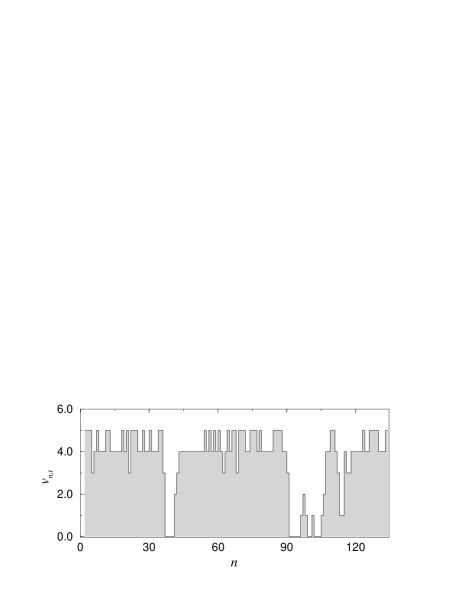
FIG. 2.: Snapshot of the velocity $v_{n,t}$ as a function of car number $n$ at a certain time $t$ and $P=0.5$. Jams are characterized by several particles with low velocity. The free flow particles fluctuate independently between $v_{n,t}=v_{\rm max}-1$ and $v_{n,t}=v_{\rm max}$.

FIG. 3.: The dynamical structure factor $S_{v}(k,\omega)$ of the velocity-particle space above the transition for $P=0.5$. Notice that the free flow phase contributes to $S_{v}(k,\omega)$ only white noise.

In the following we carry out a quantitative analysis of the ridges to obtain information about correlations between jammed particles. We will show that among those particles long range correlations exist only above the transition whereas below the transition these correlations are restricted to a finite correlation length. In Fig. 4 we plot the values of the dynamical structure factor $S_{v}(k,\omega)$ for $\omega/k=v_{\rm j}$, i.e., the values along the ridge which correspond to the jam modes. In order to take finite-size effects into account, we use the scaling ansatz

$$\left.S_{v}(k,\omega)\right|_{\omega/k=v_{\rm j}}\;=\;N^{-\theta}\,f(N^{\zeta}k).$$ (4)

For $\theta=-1.22$ and $\zeta=0.34$ we obtain a convincing data collapse of all curves. The dynamical structure factor decays algebraically,

$$\left.S_{v}(k,\omega)\right|_{\omega/k=v_{\rm j}}\;\sim\;k^{-\gamma},$$ (5)

where the exponent is given by $\gamma\approx 3.6\pm 0.2$. This algebraic decay of the dynamical structure factor indicates that the corresponding correlation function is also characterized by an algebraic decay, i.e., the system displays long range correlations above the transition. Next we are interested in the values of $S_{v}(k,\omega)$ for $\omega/k=v_{\rm j}$ below the critical density. These values are shown in Fig. 5. Due to the finite amount of standing cars below the transition, the jam mode does not vanish. Our analysis shows that the jam mode decreases like a Lorentz curve,

$$\left.S_{v}(k,\omega)\right|_{\omega/k=v_{\rm j}}\;\sim\;\frac{1}{1+(k\,\xi)^{2}}+c\,.$$ (6)

Herein $\xi$ denotes a correlation length, defined in the velocity-particle space. The term $c$ takes into consideration that, caused by the free flow phase, the jam mode does not tend to zero for large $k$ but to a finite value. Beside the jam mode, Fig. 5 shows a Lorentz curve according to Eq. (6), which has been fitted to the data. To estimate the influence of finite-size effects on the correlation length, we first determined the $\xi$ for different values of $N$ (with $T=N$) and found that $\xi$ is almost in-affected by finite-size effects for the densities shown in Fig. 5. Therefore, these values of the correlation length equal within negligible errors those values of the correlation length found in the limit $N\to\infty$ (with $N=T$). The dependence of the correlation length on $\rho_{\rm c}-\rho$ is shown in the inset of Fig. 5. With $\rho$ approaching $\rho_{\rm c}$ the correlation length diverges as

$$\xi\;\sim\;(\rho_{\rm c}-\rho)^{-\nu},$$ (7)

with $\nu=0.92\pm 0.05$.

FIG. 4.: The scaling plot of $S_{v}(k,\omega)$ along the jam mode for various values of $N$ (with $N\in\{128,256,512,1024,2048\}$ and $N=T$) and a fixed value of the global density with $\rho>\rho_{c}$. For $\theta=-1.22$ and $\zeta=0.34$ we got a good data collapse indicating that the correlation of the jams decay algebraically (dashed line with slope $\gamma=-3.6$).

Since $\xi$ describes the correlation of particles of the jammed phase, the occurrence of long range order in the system at $\rho=\rho_{\rm c}$ indicates that the system displays criticality. As mentioned above, the correlation length $\xi$ is infinite above the transition (long range order) and finite below. This coincides with measurements of the life time distribution of jams at the critical point [22] which displays a power-law behavior, i.e., traffic jams occur on all time scales. Below the critical density the life time of the jams is finite and no long range correlations of jams can occur.

FIG. 5.: The dynamical structure factor $S_{v}(k,\omega)$ for $\omega/k=v_{\rm j}$, $v_{\rm max}=5$, $P=0.5$ and $N=1024$. The dashed line corresponds to a Lorentzian fit according to Eq. (6). The inset shows the correlation length $\xi$ as a function of $\rho_{\rm c}-\rho$. The obtained power-law behavior (solid line) agrees with Eq. (7).

In the following we address the question how long range order occurs by approaching the transition point. Therefore we consider the smallest positive mode on the ridge of jammed particles, $S_{v}(k\to 0,\omega\to 0)$ with $\omega/k=v_{\rm j}$. This value contains the information how long range and long time correlations appear when the transition takes place and it is believed to be closely related to an order parameter (see for instance [23]). If the transition from the free flow regime to the jammed regime can be described as a critical phenomenon, $S_{v}(k\to 0,\omega\to 0)$ should vanish below the transition ($\rho<\rho_{c}$). Simulating finite system sizes this means that the smallest jam mode obeys the finite-size scaling ansatz

$$S_{v}(k\to 0,\omega\to 0)=(NT)^{-y/2}\,f[(NT)^{x/2}(\rho-\rho_{\rm c})],$$ (8)

with $\omega/k=v_{\rm j}$. We measured $S_{v}(k\to 0,\omega\to 0)$ for various values of $N$ and $T$ and for $P=0.321$ which corresponds to a jam velocity $v_{j}\approx-1/2$ [18]. The finite-size scaling works and for $y\approx-0.2$ and $x\approx 0.1$ we got a good data collapse, which is plotted in Fig. 6. Especially we obtain the data collapse for different ratios of $N$ and $T$, which shows that the system behaves isotropic in $N$ and $T$. To investigate the dependence of the exponents on $P$, we determined them also for another value of the noise parameter ($P=0.519$ corresponding to $v_{j}\approx-1/3$ ). Due to the size of the corresponding error bars no significant $P$ dependence of the exponents could be observed. Further investigation with improved accuracy are needed to clarify this point.

FIG. 6.: The smallest mode of $S_{v}(k\to 0,\omega\to 0)$, with $\omega/k=v_{\rm j}$, for different values of $N$ ($N\in\{128,256,512,1024\}$) and ratios $N/T$ ($N/T\in\{0.5,1,2,4\}$) and $P=0.321$.

Note that it is not justified to identify the scaling exponents [Eq. (8)] with the usual critical exponents of second order phase transitions ($y=\beta/\nu$ and $x=1/\nu$). First it is not clear if $S_{v}(k\to 0,\omega\to 0)$ equals the order parameter (see [23] and references therein). The second point is that the usual finite-size scaling ansatz rests on the validity of the hyperscaling relation between the exponents (see for instance [24]). Despite these restrictions the finite-size scaling analysis of the smallest jam mode reveals that it vanishes below the transition. In the hydrodynamic limit ($N\to\infty,T\to\infty$) no long range correlations in space and time occur for $\rho<\rho_{c}$. Above the critical value the correlation function displays an algebraic decay. Since the correlations of the jams are finite below and infinite above $\rho_{c}$ , the system displays critical behavior. This agrees with the above mentioned investigations of the life time distribution [22] of jams and with measurements of the relaxation time of the system. It was shown that the relaxation time $\tau$ diverges at the critical point with increasing system size $\tau\sim L^{z}$ with a $P$ depending exponent $z$ [15, 16, 17]. But one has to mention that above the transition the measurements of the relaxation time yields unphysical result, in the sense that the relaxation time becomes negative [17]. We think that the origin of this behavior is caused by the inhomogeneous character of the system above the transition where the system separates into two coexisting phases. The relaxation time measurement does not take this inhomogeneous character into account.

IV Conclusions

We studied numerically the Nagel-Schreckenberg traffic flow model. The investigation of the dynamical structure factor allowed us to examine the transition of the system from a free flow regime to a jammed regime. Above the transition the dynamical structure factor exhibits two modes corresponding to the coexisting free flow and jammed phase. Due to the sign of their characteristic velocities $v_{\rm f}$ and $v_{\rm j}$, both phases can clearly be distinguished.

The analysis of the dynamical structure factor of the velocity-particle space shows that above the transition the system exhibits long range correlations of the jammed particles and below the transition the correlations display a finite correlation length that diverges at the critical point, indicating that a continuous phase transition takes place. Using a finite-size scaling analysis we showed that in the hydrodynamic limit the smallest jam mode which corresponds to the long range correlations of jams vanishes below the transition. We think that an extended investigation of this quantity could lead to a convincing definition of an order parameter which describes the transition from the free flow to the jammed regime.

REFERENCES

- [1] E-mail: lars@thp.uni-duisburg.de
- [2] E-mail: sven@thp.uni-duisburg.de
- [3] E-mail: usadel@thp.uni-duisburg.de
- [4] W. Leutzbach, in Traffic and Granular Flow, edited by D. E. Wolf, M. Schreckenberg, and A. Bachem, (World Scientific, Singapore, 1996).
- [5] J. Treiterer, Appx IV to the final Report EES 202-2, Columbus Ohio State University (1965).
- [6] B. S. Kerner and H. Rehborn, Phys. Rev. E 53 1297 (1996), Phys. Rev. E 53 4275 (1996).
- [7] M. J. Lighthill and G. B. Whitham, Proc. R. Soc. London, Ser. A 229, 317 (1955).
- [8] Traffic and Granular Flow, edited by D. E. Wolf, M. Schreckenberg, and A. Bachem (World Scientific, Singapore, 1996).
- [9] Traffic and Granular Flow ’97, edited by M. Schreckenberg and D. E. Wolf (Springer, Singapore, 1998).
- [10] K. Nagel and M. Schreckenberg, J. Phys. I 2, 2221 (1992).
- [11] F. L. Hall, B. L. Allen, and M. A. Gunter, Transportation Research A 20, 197 (1986).
- [12] S. Lübeck, M. Schreckenberg, and K. D. Usadel, Phys. Rev. E 57, 1171 (1998).
- [13] D. Chowdhury, K. Ghosh, A. Majumdar, S. Sinha, and R. B. Stinchcombe, Physica A 246, 471 (1997).
- [14] L. C. Q. Vilar and A. M. C. Souza, Physica A 211, 84 (1994).
- [15] G. Csányi and J. Kertész, J. Phys. A 28, L427 (1995).
- [16] M. Sasvari and J. Kertész, Phys. Rev. E 56, 4104 (1997).
- [17] B. Eisenblätter, L. Santen, A. Schadschneider, and M. Schreckenberg, Phys. Rev. E 57, 1309 (1998).
- [18] S. Lübeck, L. Roters, and K. D. Usadel, in Traffic and Granular Flow 97, edited by M. Schreckenberg and D. E. Wolf, (Springer, Singapore, 1998).
- [19] M. Schreckenberg, A. Schadschneider, K. Nagel, and N. Ito, Phys. Rev. E 51 2939 (1995).
- [20] L. Neubert, H. Lee, and M. Schreckenberg, in Traffic and Granular Flow 97, edited by M. Schreckenberg and D. E. Wolf, (Springer, Singapore, 1998).
- [21] B. S. Kerner, S. L. Klenov, and P. Kohnhäuser, Phys. Rev. E 56 4200 (1997).
- [22] K. Nagel and M. Paczuski, Phys. Rev. E 51, 2909 (1995).
- [23] M. Schmittmann and R. K. P. Zia, in Phase Transition and Critical Phenomena, edited by C. Domb and J. L. Lebowitz, (Academic Press, London, 1995), Vol. 17.
- [24] K. Binder and D. W. Heermann, Monte Carlo Simulation in Statistical Physics, Springer Series in Solid-State Sciences 80, (Springer, Heidelberg, 1988).