Statistics of knots and entangled random walks

Abstract

The lectures review the state of affairs in modern branch of mathematical physics called probabilistic topology. In particular we consider the following problems: (i) We estimate the probability of a trivial knot formation on the lattice using the Kauffman algebraic invariants and show the connection of this problem with the thermodynamic properties of 2D disordered Potts model; (ii) We investigate the limit behavior of random walks in multi-connected spaces and on non-commutative groups related to the knot theory. We discuss the application of the above mentioned problems in statistical physics of polymer chains. On the basis of non-commutative probability theory we derive some new results in statistical physics of entangled polymer chains which unite rigorous mathematical facts with more intuitive physical arguments.

Contents

toc

I Introduction

It wouldn’t be an exaggeration to say that contemporary physical science is becoming more and more mathematical. This fact is too strongly manifested to be completely ignored. Hence I would permit myself to bring forward two possible conjectures:

(a) On the one hand there are hardly discovered any newly physical problem which would be beyond the well established methods of the modern theoretical physics. This leads to the fact that nowadays real physical problems seem to be less numerous than mathematical methods of their investigation.

(b) On the other hand the mathematical physics is a fascinating field which absorbs new ideas from different branches of modern mathematics, translates them into the physical language and hence fills the abstract mathematical constructions by the new fresh content. This ultimately leads to creating new concepts and stimulates seeking for newel deep conformities to natural laws in known physical phenomena.

The penetration of new mathematical ideas in physics has sometimes rather paradoxical character. It is not a secret that difference in means (in languages) and goals of physicists and mathematicians leads to mutual misunderstanding, making the very subject of investigation obscure. What is true for general is certainly true for particular. To clarify the point, let us turn to statistics of entangled uncrossible random walks—the well-known subject of statistical physics of polymers. Actually, since 1970s, after Conway’s works, when the first algebraic topological invariants—Alexander polynomials—became very popular in mathematical literature, physicists working in statistical topology have acquired a much more powerful topological invariant than the simple Gauss linking number. The constructive utilization of algebraic invariants in statistical physics of macromolecules has been developed in the classical works of A. Vologodskii and M. Frank-Kamenetskii [1]. However until recently in overwhelming majority of works the authors continue using the commutative Gauss invariant invariant just making references to its imperfectness.

One of the reasons of such inertia consists in the fact that new mathematical ideas are often formulated as “theorems of existence” and it takes much time to retranslate them into physically acceptable form which may serve as a real computational tool.

We intend to use some recent advances in algebraic topology and theory of random walks on non-commutative groups for reconsidering the old problem—evaluating of the entropy of randomly generated knots and entangled random walks in a given homotopic state. Let us emphasize that this is a real physical paper, and when it is possible the rigorous statements are replaced by some physically justified conjectures. Generally speaking, the work is devoted to an analysis of probabilistic problems in topology and their applications in statistical physics of polymer systems with topological constraints.

Let us formulate briefly the main results of our work.

1. The probability for a long random walk to form randomly a knot with specific topological invariant is computed. This problem is considered using the Kauffman algebraic invariants and the connection with the thermodynamic properties of 2D Potts model with “quenched” and “annealed” disorder in interaction constants is discussed.

2. The limit behavior of random walks on the non-commutative groups related to the knot theory is investigated. Namely, the connection between the limit distribution for the Lyapunov exponent of products of non-commutative random matrices—generators of “braid group”—and the asymptotic of powers (“knot complexity”) of algebraic knot invariants is established. This relation is applied for calculating the knot entropy. In particular, it is shown that the “knot complexity” corresponds to the well known topological invariant, “primitive path”, repeatedly used is statistics of entangled polymer chains.

3. The random walks on multi-connected manifolds is investigated using conformal methods and the nonabelian topological invariants are constructed. It is shown that many nontrivial properties of limit behavior of random walks with topological constraints can be explained in context of random walks on hyperbolic groups.

Usage of the limit behavior of entangled random paths established above for investigation of the statistical properties of so-called “crumpled globule” (trivial ring without self-intersections in strongly contracted state).

The connection between all these problems is shown in Table 1.

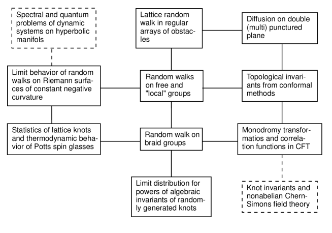
FIG. 1.: Links between topologically-probabilistic problems. Solid boxes – problems, discussed in the paper; dashed boxes – problems not included in the consideration.

II Knot diagrams as disordered spin systems

A Brief review of statistical problems in topology

The interdependence of such branches of modern theoretical and mathematical physics as theory of integrable systems, algebraic topology and conformal field theory has proved to be a powerful catalyst of development of the new direction in topology, namely, of analytical topological invariants construction by means of exactly solvable statistical models.

Today it is widely believed that the following three cornerstone findings have brought the fresh stream in topology:

— It has been found the deep relation between the Temperley-Lieb algebra and the Hecke algebra representation of the braid group. This fact resulted in the remarkable geometrical analogy between the Yang-Baxter equations, appearing as necessary condition of the transfer matrix commutativity in the theory of integrable systems on the one hand, and one of Reidemeister moves, used in the knot invariant construction on the other hand.

— It has been discovered that the partition function of the Wilson loop with the Chern-Simons action in the topological field theory coincides with the representation of the known nonabelian algebraic knot invariants written in terms of the time-ordered path integral.

— The need for new solutions of the Yang-Baxter equations has given a power impetus to the theory of quantum groups. Later on the related set of problems was separated in the independent branch of mathematical physics.

Of course the above mentioned findings do not exhaust the list of all brilliant achievements in that field during the last decade, but apparently these new accomplishments have used profound “ideological” changes in the topological science: now we can hardly consider topology as an independent branch of pure mathematics where each small step forward takes so much effort that it seems incidental.

Thus in the middle of the 80s the “quantum group” gin was released. It linked by common mathematical formalism classical problems in topology, statistical physics and field theory. A new look at the old problems and the beauty of the formulated ideas made an impression on physicists and mathematicians. As a result, in a few last years the number of works devoted to the search of the new applications of the quantum group apparatus is growing exponentially going beyond the framework of original domains. As an example of persistent penetrating of the quantum group ideas in physics we can name the works on anyon superconductivity [2], intensively discussing problems on “quantum random walks” [3], the investigation of spectral properties of “quantum deformations” of harmonic oscillators [4] and so on.

The time will show whether such “quantum group expansion” is physically justified or it merely does tribute to today’s fashion. However it is clear that physics has acquired new convenient language allowing to construct new “nonabelian objects” and to work with them.

Among the vast amount of works devoted to different aspects of the theory of integrable systems, their topological applications connected to the construction of knot and link invariants and their representation in terms of partition functions of some known 2D-models deserve our special attention. There exist several reviews [5] and books [6] on that subject and our aim by no means consists in re-interpretation or compilation of their contents. We make an attempt of consecutive account of recently solved probabilistic problems in topology as well as attract attention to some interesting, still unsolved, questions lying on the border of topology and the probability theory. Of course we employ the knowledges acquired in the algebraic topology utilizing the construction of new topological invariants done by V.F.R. Jones [5] and L.H. Kauffman [7].

Besides the traditional fundamental topological issues concerning the construction of new topological invariants, investigation of homotopic classes and fibre bundles we mark a set of adjoint but much less studied problems. First of all, we mean the problem of so-called “knot entropy” calculation. Most generally it can be formulated as follows. Take the lattice ${\rm{\sf ZZ\hskip 1.70717pt}}^{3}$ embedded in the space ${\rm{\sf RI\hskip 5.97508pt}}^{3}$. Let $\Omega_{N}$ be the ensemble of all possible closed nonselfintersecting $N$-step loops with one common fixed point on ${\rm{\sf ZZ\hskip 1.70717pt}}^{3}$; by $\omega$ we denote the particular trajectory configuration. The question is: what is the probability ${\cal P}_{N}$ of the fact that the trajectory $\omega\in\Omega_{N}$ belongs to some specific homotopic class. Formally this quantity can be represented in the following way

$$\begin{array}[]{c}{\cal P}_{N}\{\mbox{Inv}\}=\displaystyle\frac{1}{\Omega_{N}}\sum_{\{\omega\}}\Delta\left[\mbox{Inv}\{\omega\}-\mbox{Inv}\right]\equiv\vskip 6.0pt plus 2.0pt minus 2.0pt\\ \displaystyle\frac{1}{\Omega_{N}}\sum_{\{{\bf r}_{1},\ldots,{\bf r}_{N}\}}\Delta\left[\mbox{Inv}\{{\bf r}_{1},\ldots,{\bf r}_{N}\}-\mbox{Inv}\right]\Bigl{(}1-\Delta\left[{\bf r}_{i}-{\bf r}_{j}\right]\Bigr{)}\Delta\left[{\bf r}_{N}\right]\end{array}$$ (II.1)

where $\mbox{Inv}\{\omega\}$ is the functional representation of the knot invariant corresponding to the trajectory with the bond coordinates $\{{\bf r}_{1}\ldots,{\bf r}_{N}\}$; Inv is the topological invariant characterizing the knot of specific homotopic type and $\Delta(x)$ is the Kronecker function: $\Delta(x=0)=1$ and $\Delta(x\neq 0)=0$. The first $\Delta$-function in Eq.(II.1) cuts the set of trajectories with the fixed topological invariant while the second and the third $\Delta$-functions ensure the $N$-step trajectory to be nonselfintersecting and to form a closed loop respectively.

The distribution function ${\cal P}_{N}\{\mbox{Inv}\}$ satisfies the normalization condition

$$\sum_{\mbox{all homotopic classes}}P_{N}\{\mbox{Inv}\}=1$$ (II.2)

The entropy $S_{N}\{{\rm Inv}\}$ of the given homotopic state of the knot represented by $N$-step closed loop on ${\rm{\sf ZZ\hskip 1.70717pt}}^{3}$ reads

$$S_{N}\{{\rm Inv}\}=\ln\left[\Omega_{N}{\cal P}_{N}\{{\rm Inv}\}\right]$$ (II.3)

The problem concerning the knot entropy determination has been discussed time and again by the leading physicists. However the number of new analytic results in that field was insufficient till the beginning of the 80s: in about 90 percents of published materials their authors used the Gauss linking number or some of its abelian modifications for classification of a topological state of knots and links while the disadvantages of this approach were explained in the rest 10 percent of the works. We do not include in this list the celebrated investigations of A.V. Vologodskii et al [1] devoted to the first fruitful usage of the nonabelian Alexander algebraic invariants for the computer simulations in the statistical biophysics. We discuss physical applications of these topological problems at length in Section 5.

Despite of the clarity of geometrical image, the topological ideas are very hard to formalize because of the non-local character of topological constraints. Besides, the main difficulty in attempts to calculate analytically the knot entropy is due to the absence of convenient analytic representation of the complete topological invariant. Thus, to succeed, at least partially, in the knot entropy computation we simplify the general problem replacing it by the problem of calculating the distribution function for the knots with defined topological invariants. That problem differs from the original one because none of the known topological invariants (Gauss linking number, Alexander, Jones, HOMFLY) are complete. The only exception is Vassiliev invariants [8], which are beyond the scope of the present book. Strictly speaking we are unable to estimate exactly the correctness of such replacement of the homotopic class by the mentioned topological invariants. Thus under the definition of the topological state of the knot or entanglement we simply understand the determination of the corresponding topological invariant.

The problems where $\omega$ (see Eq.(II.1)) is the set of realizations of the random walk, i.e. the Markov chain are of special interest. In that case the probability to find a closed $N$-step random walk in ${\rm{\sf RI\hskip 5.97508pt}}^{3}$ in some prescribed topological state can be presented in the following way

$${\cal P}_{N}\{\mbox{Inv}\}=\int\ldots\int\prod_{j=1}^{N}d{\bf r}_{j}\prod_{j=1}^{N-1}g\left({\bf r}_{j+1}-{\bf r}_{j}\right)\delta\left[\mbox{Inv}\{{\bf r}_{1}\ldots,{\bf r}_{N}\}-\mbox{Inv}\right]\delta\left[{\bf r}_{N}\right]$$ (II.4)

where $g\left({\bf r}_{j+1}-{\bf r}_{j}\right)$ is the probability to find $j+1$th step of the trajectory in the point ${\bf r}_{j+1}$ if $j$th step is in ${\bf r}_{j}$. In the limit $a\to 0$ and $N\to\infty$ ($Na=L=\mbox{const}$) in three-dimensional space we have the following expression for $g\left({\bf r}_{j+1}-{\bf r}_{j}\right)$

$$g\left({\bf r}_{j+1}-{\bf r}_{j}\right)=\left(\frac{3}{2\pi a^{2}}\right)^{3/2}\exp\left(-\frac{3({\bf r}_{j+1}-{\bf r}_{j})^{2}}{2a^{2}}\right)\simeq\left(\frac{3}{2\pi a^{2}}\right)^{3/2}\exp\left\{\frac{3}{2a}\left(\frac{d{\bf r}(s)}{ds}\right)^{2}\right\}$$ (II.5)

Introducing the “time”, $s$, along the trajectory we rewrite the distribution function ${\cal P}_{N}\{\mbox{Inv}\}$ (Eq.(II.4)) in the path integral form with the Wiener measure density

$${\cal P}_{N}\{\mbox{Inv}\}=\frac{1}{\cal Z}\int\ldots\int{\cal D}\{{\bf r}\}\exp\left\{-\frac{3}{2a}\int_{0}^{L}\left(\frac{d{\bf r}(s)}{ds}\right)^{2}ds\right\}\delta[\mbox{Inv}\{{\bf r}(s)\}-\mbox{Inv}]$$ (II.6)

and the normalization condition is as follows

$${\cal Z}=\sum_{\begin{array}[]{c}\mbox{all different}\vspace{-3mm}\\ \mbox{knot invariants}\end{array}}{\cal P}_{N}\{\mbox{Inv}\}$$

The form of Eq.(II.6) up to the Wick turn and the constants coincides with the scattering amplitude $\alpha$ of a free quantum particle in the multi-connected phase space. Actually, for the amplitude $\alpha$ we have

$$\alpha\sim\sum_{\begin{array}[]{c}\mbox{all paths from given}\vspace{-3mm}\\ \mbox{topological class}\end{array}}\exp\left\{\frac{i}{h}\int\dot{\bf r}^{2}(s)ds\right\}$$ (II.7)

If phase trajectories can be mutually transformed by means of continuous deformations, then the summation in Eq.(II.7) should be extended to all available paths in the system, but if the phase space consists of different topological domains, then the summation in Eq.(II.7) refers to the paths from the exclusively defined class and the “knot entropy” problem arises.

B Abelian problems in statistics of entangled random walks and incompleteness of Gauss invariant

As far back as 1967 S.F. Edwards had discovered the basis of the statistical theory of entanglements in physical systems. In [9] he proposed the way of exact calculating the partition function of self-intersecting random walk topologically interacting with the infinitely long uncrossible string (in 3D case) or obstacle (in 2D-case). That problem had been considered in mathematical literature even earlier—see the paper [10] for instance—but S.F. Edwards was apparently the first to recognize the deep analogy between abelian topological problems in statistical mechanics of the Markov chains and quantum-mechanical problems (like Bohm-Aharonov) of the particles in the magnetic fields. The review of classical results is given in [12], whereas some modern advantages are discussed in [11].

The 2D version of the Edwards’ model is formulated as follows. Take a plane with an excluded origin, producing the topological constraint for the random walk of length $L$ with the initial and final points ${\bf r}_{0}$ and ${\bf r}_{L}$ respectively. Let trajectory make $n$ turns around the origin (fig.2). The question is in calculating the distribution function ${\cal P}_{n}({\bf r}_{0},{\bf r}_{L},L)$.

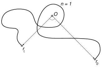
FIG. 2.: Random walk on the plane near the single obstacle.

In the said model the topological state of the path $C$ is fully characterized by number of turns of the path around the origin. The corresponding abelian topological invariant is known as Gauss linking number and when represented in the contour integral form, reads

$$\mbox{Inv}\{{\bf r}(s)\}\equiv G\{C\}=\int_{C}\frac{ydx-xdy}{x^{2}+y^{2}}=\int_{C}{\bf A}({\bf r})d{\bf r}\equiv 2\pi n+\vartheta$$ (II.8)

where

$${\bf A}({\bf r})={\bf\xi}\times\frac{{\bf r}}{r^{2}};\qquad{\bf\xi}=(0,0,1)$$ (II.9)

and $\vartheta$ is the angle distance between ends of the random walk.

Substituting Eq.(II.8) into Eq.(II.6) and using the Fourier transform of the $\delta$-function, we arrive at

$${\cal P}_{n}({\bf r}_{0},{\bf r}_{L},L)=\frac{1}{\pi La}\exp\left(\frac{r_{0}^{2}+r_{L}^{2}}{La}\right)\int_{-\infty}^{\infty}I_{|\lambda|}\left(\frac{2r_{0}r_{L}}{La}\right)e^{i\lambda(2\pi n+\vartheta)}d\lambda$$ (II.10)

which reproduces the well known old result [9] (some very important generalizations one can find in [11]).

Physically significant quantity obtained on the basis of Eq.(II.10) is the entropic force

$$f_{n}(\rho)=-\frac{\partial}{\partial\rho}\ln{\cal P}_{n}(\rho,L)$$ (II.11)

which acts on the closed chain $({\bf r}_{0}={\bf r}_{L}=\rho,\;\vartheta=0)$ when the distance between the obstacle and a certain point of the trajectory changes. Apparently the topological constraint leads to the strong attraction of the path to the obstacle for any $n\neq 0$ and to the weak repulsion for $n=0$.

Another exactly solvable 2D-problem closely related to the one under discussion deals with the calculation of the partition function of a random walk with given algebraic area. The problem concerns the determination of the distribution function ${\cal P}_{S}({\bf r}_{0},{\bf r}_{L},L)$ for the random walk with the fixed ends and specific algebraic area $S$.

As a possible solution of that problem, D.S. Khandekar and F.W. Wiegel [13] again represented the distribution function in terms of the path integral Eq.(II.6) with the replacement

$$\delta[\mbox{Inv}\{{\bf r}(s)\}-\mbox{Inv}]\to\delta[S\{{\bf r}(s)\}-S]$$ (II.12)

where the area is written in the Landau gauge:

$$S\{{\bf r}(s)\}=\frac{1}{2}\int_{C}ydx-xdy=\frac{1}{2}\int_{C}\tilde{\bf A}\{{\bf r}\}\dot{\bf r}ds;\qquad\tilde{\bf A}=\xi\times{\bf r}$$ (II.13)

(compare to Eqs.(II.8)-(II.9)).

The final expression for the distribution function reads ([12])

$${\cal P}_{S}({\bf r}_{0},{\bf r}_{L},L)=\frac{1}{2\pi}\int_{-\infty}^{\infty}dg\;e^{iqS}\;{\cal P}_{q}({\bf r}_{0},{\bf r}_{L},L)$$ (II.14)

where

$$\begin{array}[]{l}\displaystyle{\cal P}_{q}({\bf r}_{0},{\bf r}_{L},L)=\frac{\lambda}{4\pi\sin\frac{La\lambda}{4}}\\ \displaystyle\qquad\times\exp\left\{\frac{\lambda}{2}(x_{0}y_{L}-y_{0}x_{L})-\frac{\lambda}{4}\left((x_{L}-x_{0})^{2}+(y_{L}-y_{0})^{2}\right)\cot\frac{La\lambda}{4}\right\}\end{array}$$ (II.15)

and $\lambda=-iq$.

For closed trajectories Eqs.(II.14)-(II.15) can be simplified essentially, giving

$${\cal P}_{S}^{cl}(N)=2La\cosh^{2}\left(\frac{2\pi S}{La}\right)$$ (II.16)

Different aspects of this problem have been extensively studied in [11].

There is no principal difference between the problems of random walk statistics in the presence of a single topological obstacle or with a fixed algebraic area—both of them have the “abelian” nature. Nevertheless we would like to concentrate on the last problem because of its deep connection with the famous Harper-Hofstadter model dealing with spectral properties of the 2D electron hopping on the discrete lattice in the constant magnetic field [14]. Actually, rewrite Eq.(II.4) with the substitution Eq.(II.12) in form of recursion relation in the number of steps, $N$:

$$\begin{array}[]{c}\displaystyle{\cal P}_{q}({\bf r}_{N+1},N+1)=\int d{\bf r}_{N}g\left({\bf r}_{N+1}-{\bf r}_{N}\right)\exp\left(\frac{iq}{2}{\bf\xi}({\bf r}_{N}\times{\bf r}_{N+1})\right)\vskip 6.0pt plus 2.0pt minus 2.0pt\\ \displaystyle\times{\cal P}_{q}({\bf r}_{N},N)\end{array}$$ (II.17)

For the discrete random walk on ${\rm{\sf ZZ\hskip 1.70717pt}}^{2}$ we use the identity

$$\int d{\bf r}_{N}g\left({\bf r}_{N+1}-{\bf r}_{N}\right)(\ldots)\to\sum_{\{{\bf r}_{N}\}}w\left({\bf r}_{N+1}-{\bf r}_{N}\right)(\ldots)$$ (II.18)

where $w\left({\bf r}_{N+1}-{\bf r}_{N}\right)$ is the matrix of the local jumps on the square lattice; $w$ is supposed to be symmetric:

$$w=\left\{\begin{array}[]{cl}\frac{1}{4}&\mbox{for $(x,y)\to(x,y\pm 1)$ and $(x,y)\to(x\pm 1,y)$}\vskip 6.0pt plus 2.0pt minus 2.0pt\\ 0&\mbox{otherwise}\end{array}\right.$$ (II.19)

Finally, we get in the Landau gauge:

$$\begin{array}[]{lll}\displaystyle\frac{4}{\varepsilon}W(x,y,q,\varepsilon)&=&\displaystyle e^{\frac{1}{2}iqx}W(x,y-1,q)+\displaystyle e^{-\frac{1}{2}iqx}W(x,y+1,q)\;+\vskip 6.0pt plus 2.0pt minus 2.0pt\\ &&\displaystyle e^{\frac{1}{2}iqy}W(x-1,y,q)+e^{-\frac{1}{2}iqy}W(x+1,y,q)\end{array}$$ (II.20)

where $W(x,y,q,\varepsilon)$ is the generating function defined via relation

$$W(x,y,q,\varepsilon)=\sum_{N=0}^{\infty}\varepsilon^{N}{\cal P}_{S}({\bf r}_{N},N)$$

and $q$ plays a role of the magnetic flux through the contour bounded by the random walk on the lattice.

There is one point which is still out of our complete understanding. On the one hand the continuous version of the described problem has very clear abelian background due to the use of commutative “invariants” like algebraic area Eq.(II.13). On the other hand it has been recently discovered ([15]) that so-called Harper equation, i.e. Eq.(II.20) written in the gauge $S\{{\bf r}\}=\int_{C}ydx$, exhibits the hidden quantum group symmetry related to the so-called $C^{*}$–algebra ([16]) which is strongly nonabelian. Usually in statistical physics we expect that the continuous limit (when lattice spacing tends to zero with corresponding rescaling of parameters of the model) of any discrete problem does not change the observed physical picture, at least qualitatively. But for the considered model the spectral properties of the problem are extremely sensitive to the actual physical scale of the system and depend strongly on the lattice geometry.

The generalization of the above stated problems concerns, for instance, the computation of the partition function for the random walk entangled with $k>1$ obstacles on the plane located in the points $\{{\bf r}_{1},\ldots,{\bf r}_{k}\}$. At first sight, approach based on usage of Gauss linking number as topological invariant, might allow us to solve such problem easily. Let us replace the vector potential ${\bf A}({\bf r})$ in Eq.(II.8) by the following one

$${\bf A}({\bf r}_{1},\ldots,{\bf r}_{k})={\bf\xi}\times\sum_{j=1}^{k}\frac{{\bf r}-{\bf r}_{j}}{|{\bf r}-{\bf r}_{j}|^{2}}$$ (II.21)

The topological invariant in this case will be the algebraic sum of turns around obstacles, which seems to be a natural generalization of the Gauss linking number to the case of many-obstacle entanglements.

However, the following problem is bound to arise: for the system with two or more obstacles it is possible to imagine closed trajectories entangled with a few obstacles together but not entangled with every one. In the fig.3 the so-called “Pochhammer contour” is shown. Its topological state with respect to the obstacles cannot be described using any abelian version of the Gauss-like invariants.

FIG. 3.: Pochammer contour entangled with two obstacles together but not entangled with every one.

To clarify the point we can apply to the concept of the homotopy group [17]. Consider the topological space ${\cal R}={\rm{\sf RI\hskip 5.97508pt}}^{2}-\{{\bf r}_{1},{\bf r}_{2}\}$ where $\{{\bf r}_{1},{\bf r}_{2}\}$ are the coordinates of the removed points (obstacles) and choose an arbitrary reference point ${\bf r}_{0}$. Consider the ensemble of all directed trajectories starting and finishing in the point ${\bf r}_{0}$. Take the basis loops $\gamma_{1}(s)$ and $\gamma_{2}(s)$ $(0<s<L)$ representing the right-clock turns around the points ${\bf r}_{1}$ and ${\bf r}_{2}$ respectively. The same trajectories passed in the counter-clock direction are denoted by $\gamma^{-1}_{1}(s)$ and $\gamma^{-1}_{2}(s)$.

The multiplication of the paths is their composition: for instance, $\gamma_{1}\gamma_{2}=\gamma_{1}\circ\gamma_{2}$. The unit (trivial) path is the composition of an arbitrary loop with its inverse:

$$e=\gamma_{i}\gamma_{i}^{-1}=\gamma_{i}^{-1}\gamma_{i}\qquad\qquad i=\{1,2\}.$$ (II.22)

The loops $\gamma_{i}(s)$ and $\tilde{\gamma}_{i}(s)$ are called equivalent if one can be transformed into another by means of monotonic change of variables $s=s(\tilde{s})$. The homotopic classes of directed trajectories form the group with respect to the paths multiplication; the unity is the homotopic class of the trivial paths. This group is known as the homotopy group $\pi_{1}({\cal R},{\bf r}_{0})$.

Any closed path on ${\cal R}$ can be represented by the “word” consisting of set of letters $\{\gamma_{1},\gamma_{2},\gamma_{1}^{-1},\gamma_{2}^{-1}\}$. Taking into account Eq.(II.22), we can reduce each word to the minimal irreducible representation. For example, the word $W=\gamma_{1}\gamma_{2}^{-1}\gamma_{1}\gamma_{1}\gamma_{1}^{-1}\gamma_{2}^{-1}\gamma_{2}\gamma_{1}^{-1}\gamma_{2}^{-1}$ can be transformed to the irreducible form: $W=\gamma_{1}\gamma_{2}^{-1}\gamma_{2}^{-1}$. It is easy to understand that the word $W\equiv e$ represents only the unentangled contours. The entanglement in fig.3 corresponds to the irreducible word $W=\gamma_{1}^{-1}\gamma_{2}\gamma_{1}\gamma_{2}^{-1}\equiv 1$. The non-abelian character of the topological constraints is reflected in the fact that different entanglements do not commute: $\gamma_{1}\gamma_{2}\neq\gamma_{2}\gamma_{1}$. At the same time, the total algebraic number of turns (Gauss linking number) for the path in fig.3 is equal to zero, i.e. it belongs to the trivial class of homology. Speaking more formally, the mentioned example is the direct consequence of the well known fact in topology: the classes of homology of knots (of entanglements) do not coincide in general with the corresponding homotopic classes. The first ones for the group $\pi_{1}$ can be distinguished by the Gauss invariant, while the problem of characterizing the homotopy class of a knot (entanglement) by an analytically defined invariant is one of the main problems in topology.

The principal difficulty connected with application of the Gauss invariant is due to its incompleteness. Hence, exploiting the abelian invariants for adequate classification of topologically different states in the systems with multiple topological constraints is very problematic.

C Nonabelian Algebraic Knot Invariants

The most obvious topological questions concerning the knotting probability during the random closure of the random walk cannot be answered using the Gauss invariant due to its weakness.

The break through in that field was made in 1975-1976 when the algebraic polynomials were used for the topological state identification of closed random walks generated by the Monte-Carlo method [1]. It has been recognized that the Alexander polynomials being much stronger invariants than the Gauss linking number, could serve as a convenient tool for the calculation of the thermodynamic properties of entangled random walks. That approach actually appeared to be very fruitful and the main part of our modern knowledge on knots and links statistics is obtained with the help of these works and their subsequent modifications.

In the present Section we develop the analytic approach in statistical theory of knots considering the basic problem—the probability to find a randomly generated knot in a specific topological state. We would like to reiterate that our investigation would be impossible without utilizing of algebraic knot invariants discovered recently. Below we reproduce briefly the construction of Jones invariants following the Kauffman approach in the general outline.

1 Disordered Potts model and generalized dichromatic polynomials

The graph expansion for the Potts model with the disorder in the interaction constants can be defined by means of slight modification of the well known construction of the ordinary Potts model [18, 19]. Let us recall the necessary definitions.

Take an arbitrary graph ${\cal L}$ with $N$ vertices. To each vertex of the given graph we attribute the “spin” variable ${\bf\sigma}_{i}$ $(i\in[1,N])$ which can take $q$ states labelled as $1,2,\ldots,q$ on the simplex. Suppose that the interaction between spins belonging to the connected neighboring graph vertices only contributes to the energy. Define the energy of the spin’s interaction as follows

$$E_{kl}=J_{kl}\,\delta({\bf\sigma}_{k},{\bf\sigma}_{l})=\cases{J_{kl}&${\bf\sigma}_{k}={\bf\sigma}_{l},\;({\bf\sigma}_{k},{\bf\sigma}_{l})$ -- neighbors \vskip 6.0pt plus 2.0pt minus 2.0pt\cr 0&otherwise}$$ (II.23)

where $J_{kl}$ is the interaction constant which varies for different graph edges and the equality ${\bf\sigma}_{k}={\bf\sigma}_{l}$ means that the neighboring spins take equal values on the simplex.

The partition function of the Potts model now reads

$$Z_{potts}=\sum_{\{{\bf\sigma}\}}\exp\left\{\sum_{\{kl\}}\frac{J_{kl}}{T}\delta({\bf\sigma}_{k},{\bf\sigma}_{l})\right\}$$ (II.24)

where $T$ is the temperature.

Expression Eq.(II.24) gives for $q=2$ the well-known representation of the Ising model with the disordered interactions extensively studied in the theory of spin glasses [20]. (Later on we would like to fill in this old story by a new “topological” sense.)

To proceed with the graph expansion of the Potts model [19], rewrite the partition function (II.24) in the following way

$$Z_{potts}=\sum_{\{{\bf\sigma}\}}\prod_{\{kl\}}\left[1+v_{kl}\;\delta({\bf\sigma}_{k},{\bf\sigma}_{l})\right]$$ (II.25)

where

$$v_{kl}=\exp\left(\frac{J_{kl}}{T}\right)-1$$ (II.26)

If the graph ${\cal L}$ has $N$ edges then the product Eq.(II.25) contains $N$ multipliers. Each multiplier in that product consists of two terms $\{1$ and $v_{kl}\,\delta({\bf\sigma}_{k},{\bf\sigma}_{l})\}$. Hence the partition function Eq.(II.25) is decomposed in the sum of $2^{N}$ terms.

Each term in the sum is in one-to-one correspondence with some part of the graph ${\cal L}$. To make this correspondence clearer, it should be that an arbitrary term in the considered sum represents the product of $N$ multipliers described above in ones from each graph edge. We accept the following convention:

(a) If for some edge the multiplier is equal to $1$, we remove the corresponding edge from the graph ${\cal L}$;

(b) If the multiplier is equal to $v_{kl}\,\delta({\bf\sigma}_{k},{\bf\sigma}_{l})$ we keep the edge in its place.

After repeating the same procedure with all graph edges, we find the unique representation for all terms in the sum Eq.(II.25) by collecting the components (either connected or not) of the graph ${\cal L}$.

Take the typical graph $G$ consisting of $m$ edges and $C$ connected components where the separated graph vertex is considered as one component. The presence of $\delta$-functions ensures the spin’s equivalence within one graph component. As a result after summation of all independent spins and of all possible graph decompositions we get the new expression for the partition function of the Potts system Eq.(II.24)

$$Z_{potts}=\sum_{\{G\}}q^{C}\prod_{\{kl\}}^{m}v_{kl}$$ (II.27)

where the product runs over all edges in the fixed graph $G$.

It should be noted that the graph expansion Eq.(II.27) where $v_{kl}\equiv v$ for all $\{k,l\}$ coincides with the well known representation of the Potts system in terms of dichromatic polynomial (see, for instance, [18, 19]).

Another comment concerns the number of spin states, $q$. As it can be seen, in the derivation presented above we did not account for the fact that $q$ has to take positive integer values only. From this point of view the representation Eq.(II.27) has an advantage with respect to the standard representation Eq.(II.24) and can be considered an analytic continuation of the Potts system to the non-integer and even complex values of $q$. We show in the subsequent sections how the defined model is connected to the algebraic knot invariants.

2 Reidemeister Moves and State Model for Construction of Algebraic Invariants

Let $K$ be a knot (or link) embedded in the 3D-space. First of all we project the knot (link) onto the plane and obtain the 2D-knot diagram in the so-called general position (denoted by $K$ as well). It means that only the pair crossings can be in the points of paths intersections. Then for each crossing we define the passages, i.e. parts of the trajectory on the projection going “below” and “above” in accordance with its natural positions in the 3D-space.

For the knot plane projection with defined passages the following theorem is valid: (Reidemeister [22]):

Two knots embedded in ${\rm{\sf RI\hskip 5.97508pt}}^{3}$ can be deformed continuously one into the other if and only if the diagram of one knot can be transformed into the diagram corresponding to another knot via the sequence of simple local moves of types I, II and III shown in fig.4.

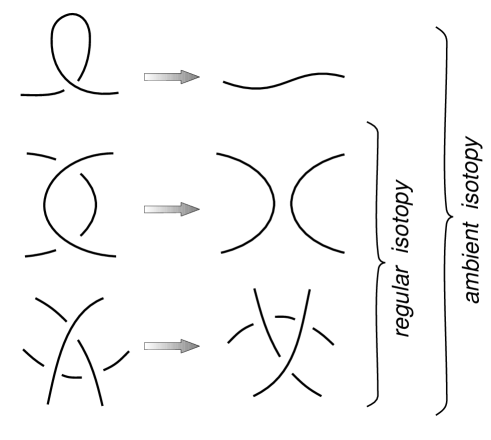
FIG. 4.: Reidemeister moves of types I, II and III.

The work [22] provides us with the proof of this theorem. Two knots are called regular isotopic if they are isotopic with respect to two last Reidemeister moves (II and III); meanwhile, if they are isotopic with respect to all moves, they are called ambient isotopic. As it can be seen from fig.4, the Reidemeister move of type I leads to the cusp creation on the projection. At the same time it should be noted that all real 3D-knots (links) are of ambient isotopy.

Now, after the Reidemeister theorem has been formulated, it is possible to describe the construction of polynomial “bracket” invariant in the way proposed by L.H. Kauffman [7, 23]. This invariant can be introduced as a certain partition function being the sum over the set of some formal (“ghost”) degrees of freedom.

Let us consider the 2D-knot diagram with defined passages as a certain irregular lattice (graph). Crossings of path on the projection are the lattice vertices. Turn all these crossings to the standard positions where parts of the trajectories in each graph vertex are normal to each other and form the angles of $\pm\pi/4$ with the $x$-axis. It can be proven that the result does not depend on such standardization.

There are two types of vertices in our lattice—a) and b) which we label by the variable $b_{i}=\pm 1$ as it is shown below:

$$\mbox{(a)}\quad\;\begin{picture}(10.0,10.0) \put(0.0,-3.5){\line(1,1){4.0}} \put(6.0,2.5){\line(1,1){4.0}} \put(10.0,-3.5){\line(-1,1){10.0}} \end{picture}\quad b_{i}=+1\quad\qquad\mbox{and}\quad\qquad\mbox{(b)}\quad\;\begin{picture}(10.0,10.0) \put(0.0,-3.5){\line(1,1){10.0}} \put(10.0,-3.5){\line(-1,1){4.0}} \put(4.0,2.5){\line(-1,1){4.0}} \end{picture}\quad b_{i}=-1$$

The next step in the construction of algebraic invariant is introduction of two possible ways of vertex splittings. Namely, we attribute to each way of graph splitting the following statistical weights: $A$ to the horizontal splitting and $B$ to the vertical one for the vertex of type a); $B$ to the horizontal splitting and $A$ to the vertical one for the vertex of type b). The said can be schematically reproduced in the following picture:

the constants $A$ and $B$ to be defined later.

For the knot diagram with $N$ vertices there are $2^{N}$ different microstates, each of them representing the set of splittings of all $N$ vertices. The entire microstate, $S$, corresponds to the knot (link) disintegration to the system of disjoint and non-selfintersecting circles. The number of such circles for the given microstate $S$ we denote as ${\cal S}$. The following statement belongs to L. Kauffman ([7]).

Consider the partition function

$$\left<K\right>=\sum_{\{S\}}d^{{\cal S}-1}A^{i}B^{j},$$ (II.28)

where $\sum_{\{S\}}$ means summation over all possible $2^{N}$ graph splittings, $i$ and $j=N-i$ being the numbers of vertices with weights $A$ and $B$ for the given realization of all splittings in the microstate $S$ respectively.

The polynomial in $A$, $B$ and $d$ represented by the partition function Eq.(II.28) is the topological invariant of knots of regular isotopy if and only if the following relations among the weights $A$, $B$ and $d$ are fulfilled:

$$\begin{array}[]{r}AB=1\vskip 6.0pt plus 2.0pt minus 2.0pt\\ ABd+A^{2}+B^{2}=0\end{array}$$ (II.29)

The sketch of the proof is as follows. Denote with $\left<\ldots\right>$ the statistical weight of the knot or of its part. The $\left<K\right>$-value equals the product of all weights of knot parts. Using the definition of vertex splittings, it is easy to test the following identities valid for unoriented knot diagrams

$$\begin{array}[]{ccl}\left<\;\begin{picture}(10.0,10.0) \put(0.0,-3.5){\line(1,1){4.0}} \put(6.0,2.5){\line(1,1){4.0}} \put(10.0,-3.5){\line(-1,1){10.0}} \end{picture}\right>&=&\left<\;\begin{picture}(7.0,12.5) \put(3.5,-3.3){\oval(7.0,7.0)[t]} \put(3.5,5.5){\oval(7.0,7.0)[b]} \end{picture}\;\right>\;A\;+\;\left<\;\begin{picture}(12.5,6.5) \put(0.0,1.0){\oval(7.0,7.0)[r]} \put(9.0,1.0){\oval(7.0,7.0)[l]} \end{picture}\right>\;B\\ \left<\;\begin{picture}(10.0,10.0) \put(0.0,-3.5){\line(1,1){10.0}} \put(10.0,-3.5){\line(-1,1){4.0}} \put(4.0,2.5){\line(-1,1){4.0}} \end{picture}\right>&=&\left<\;\begin{picture}(7.0,12.5) \put(3.5,-3.3){\oval(7.0,7.0)[t]} \put(3.5,5.5){\oval(7.0,7.0)[b]} \end{picture}\;\right>\;B\;+\;\left<\;\begin{picture}(12.5,6.5) \put(0.0,1.0){\oval(7.0,7.0)[r]} \put(9.0,1.0){\oval(7.0,7.0)[l]} \end{picture}\right>\;A\end{array}$$ (II.30)

completed by the “initial condition”

$$\Bigl{<}K\bigcup O\Bigr{>}=d\Bigl{<}K\Bigr{>};\qquad\mbox{$K$ is not empty}$$ (II.31)

where $O$ denotes the separated trivial loop.

The skein relations Eq.(II.30) correspond to the above defined weights of horizontal and vertical splittings while the relation Eq.(II.31) defines the statistical weights of the composition of an arbitrary knot and a single trivial ring. These diagrammatic rules are well defined only for fixed “boundary condition” of the knot (i.e., for the fixed part of the knot outside the brackets). Suppose that by convention the polynomial of the trivial ring is equal to the unity;

$$\Bigl{<}O\Bigr{>}=1$$ (II.32)

Now it can be shown that under the appropriate choice of the relations between $A$, $B$ and $d$, the partition function Eq.(II.28) represents the algebraic invariant of the knot. The proof is based on direct testing of the invariance of $\left<K\right>$-value with respect to the Reidemeister moves of types II and III. For instance, for the Reidemeister move of type II we have:

$$\begin{array}[]{c}\left<\;\begin{picture}(10.0,10.0)\put(10.0,1.0){\oval(10.0,12.0)[l]} \put(8.0,1.0){\oval(4.0,8.0)[r]} \put(4.0,5.0){\line(-1,0){3.0}} \put(4.0,-3.0){\line(-1,0){3.0}} \end{picture}\;\;\right>=\left<\begin{picture}(11.0,12.0)\put(6.0,-2.0){\line(-3,-2){5.0}} \put(6.0,-2.0){\line(3,-2){5.0}} \put(6.0,1.0){\circle{3.0}} \put(11.0,7.0){\line(-3,-2){5.0}} \put(1.0,7.0){\line(3,-2){5.0}} \end{picture}\;\right>\;ABd\;+\;\left<\;\begin{picture}(12.0,10.0)\put(6.0,0.5){\oval(4.0,3.0)[t]} \put(7.0,0.5){\oval(2.0,2.0)[rb]} \put(5.0,0.5){\oval(2.0,2.0)[lb]} \put(5.0,-0.5){\line(-3,-2){5.0}} \put(7.0,-0.5){\line(3,-2){5.0}} \put(6.0,3.0){\line(2,1){6.0}} \put(6.0,3.0){\line(-2,1){6.0}} \end{picture}\;\right>\;B^{2}\;+\\ \left<\;\begin{picture}(12.0,10.44)\put(0.0,-3.9){\line(2,1){6.0}} \put(12.0,-3.9){\line(-2,1){6.0}} \put(6.0,1.75){\oval(4.0,3.0)[b]} \put(5.0,1.75){\oval(2.0,2.0)[lt]} \put(7.0,1.75){\oval(2.0,2.0)[rt]} \put(11.89,6.25){\line(-3,-2){5.0}} \put(0.0,6.25){\line(3,-2){5.0}} \end{picture}\;\right>\;A^{2}\;+\;\left<\;\begin{picture}(12.0,10.33)\put(5.0,-1.0){\line(-3,-2){5.0}} \put(7.5,-1.0){\line(3,-2){5.0}} \put(5.0,1.0){\oval(4.0,4.0)[l]} \put(7.5,1.0){\oval(3.0,4.0)[r]} \put(0.0,6.3){\line(3,-2){5.0}} \put(12.5,6.3){\line(-3,-2){5.0}} \end{picture}\;\right>\;AB=\;\;\left<\;\begin{picture}(7.0,12.5) \put(3.5,-3.3){\oval(7.0,7.0)[t]} \put(3.5,5.5){\oval(7.0,7.0)[b]} \end{picture}\;\right>\;\left(ABd+A^{2}+B^{2}\right)\;+\;\left<\;\begin{picture}(12.5,6.5) \put(0.0,1.0){\oval(7.0,7.0)[r]} \put(9.0,1.0){\oval(7.0,7.0)[l]} \end{picture}\right>\;AB\end{array}$$ (II.33)

Therefore, the invariance with respect to the Reidemeister move of type II can be obtained immediately if we set the statistical weights in the last line of Eq.(II.33) as it is written in Eq.(II.29). Actually, the topological equivalence of two knot diagrams is restored with respect to the Reidemeister move of type II only if the right- and left-hand sides of Eq.(II.33) are identical. It can also be tested that the condition of obligatory invariance with respect to the Reidemeister move of type III does not violate the relations Eq.(II.29).

The relations Eq.(II.29) can be converted into the form

$$B=A^{-1},\qquad d=-A^{2}-A^{-2}$$ (II.34)

which means that the Kauffman invariant Eq.(II.28) is the Laurent polynomial in $A$-value only.

Finally, Kauffman showed that for oriented knots (links) the invariant of ambient isotopy (i.e., the invariant with respect to all Reidemeister moves) is defined via relation:

$$f[K]=(-A)^{3Tw(K)}\left<K\right>$$ (II.35)

here $Tw(K)$ is the twisting of the knot (link), i.e. the sum of signs of all crossings defined by the convention:

(not to be confused with the definition of the variable $b_{i}$ introduced above). Eq.(II.35) follows from the following chain of equalities

$$\begin{array}[]{lll}f\left[\;\;\begin{picture}(14.0,6.0)\put(13.0,6.0){\vector(-1,-1){10.0}} \put(7.0,2.0){\line(-1,1){4.0}} \put(9.0,0.0){\vector(1,-1){4.0}} \put(3.0,1.0){\oval(9.0,10.0)[l]} \end{picture}\right]&=&\left<\;\begin{picture}(14.0,8.0)\put(15.0,7.0){\line(-1,-1){5.0}} \put(10.0,2.0){\line(-1,1){5.0}} \put(15.0,-5.0){\line(-1,1){5.0}} \put(10.0,0.0){\line(-1,-1){5.0}} \put(5.0,1.0){\oval(11.0,12.0)[l]} \end{picture}\right>\;B\;+\left<\begin{picture}(15.0,8.0)\put(13.0,1.0){\oval(9.0,10.0)[l]} \put(4.0,1.0){\oval(6.0,10.0)} \end{picture}\right>\;dA\\ &=&\left<\begin{picture}(8.0,8.0)\put(5.0,1.0){\oval(9.0,10.0)[l]} \end{picture}\right>\;(B+dA)\;\equiv\;\left<\begin{picture}(8.0,8.0)\put(5.0,1.0){\oval(9.0,10.0)[l]} \end{picture}\right>(-A)^{3}\end{array}$$

The state model and bracket polynomials introduced by L.H. Kauffman seem to be very special. They explore only the peculiar geometrical rules such as summation over the formal “ghost” degrees of freedom—all possible knot (link) splittings with simple defined weights. But one of the main advantages of the described construction is connected with the fact that Kauffman polynomials in $A$-value coincide with Jones knot invariants in $t$-value (where $t=A^{1/4}$).

Jones polynomial knot invariants were discovered first by V.F.R. Jones during his investigation of topological properties of braids (see Section 3 for details). Jones’ proposition concerns the establishment of the deep connection between the braid group relations and the Yang-Baxter equations ensuring the necessary condition of transfer matrix commutativity [6]. The Yang-Baxted equations play an exceptionally important role in the statistical physics of integrable systems (such as ice, Potts, $O(n)$, 8-vertex, quantum Heisenberg models [19]).

The attempt to apply Kauffman invariants of regular isotopy for investigation of statistical properties of random walks with topological constraints in a thin slit has been made recently [24]. Below we extend the ideas of the work [24] considering the topological state of the knot as a special kind of a quenched disorder.

D Lattice knot diagrams as disordered Potts model

Let us specify the model under consideration. Take a square lattice ${\cal M}$ turned to the angle $\pi/4$ with respect to the $x$-axis and project a knot embedded in ${\rm{\sf RI\hskip 5.97508pt}}^{3}$ onto ${\cal M}$ supposing that each crossing point of the knot diagram coincides with one lattice vertex without fall (there are no empty lattice vertices)—see fig.5. Define the passages in all $N$ vertices and choose such boundary conditions which ensure the lattice to form a single closed path; that is possible when $\sqrt{N}$ (i.e. $N$) is an odd number. The frozen pattern of all passages $\{b_{i}\}$ on the lattice together with the boundary conditions fully determine the topology of some 3D knot.

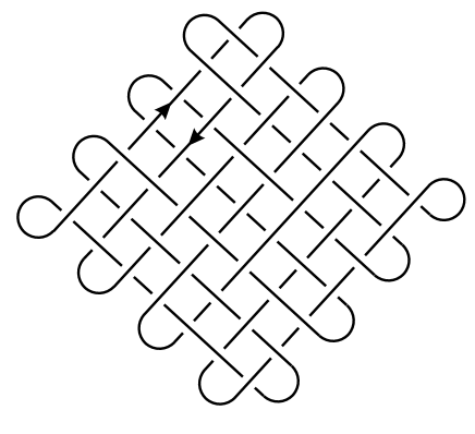
FIG. 5.: Lattice knot with topological disorder realized in a quenched random pattern of passages.

Of course, the model under consideration is rather rough because we neglect the “space” degrees of freedom due to trajectory fluctuations and keep the pure topological specificity of the system. Later on in Chapter 4 we discuss the applicability of such model for real physical systems and produce arguments in support of its validity.

The basic question of our interest is as follows: what is the probability ${\cal P}_{N}\{f[K]\}$ to find a knot diagram on our lattice ${\cal M}$ in a topological state characterized by some specific Kauffman invariant $f[K]$ among all $2^{N}$ microrealizations of the disorder $\{b_{i}\}$ in the lattice vertices. That probability distribution reads (compare to Eq.(II.1))

$${\cal P}_{N}\{f[K]\}=\frac{1}{2^{N}}\sum_{\{b_{i}\}}\Delta\Bigl{[}f[K\{b_{1},b_{2},\ldots,b_{N}\}]-f[K]\Bigr{]}$$ (II.36)

where $f[K\{b_{1},\ldots,b_{N}\}]$ is the representation of the Kauffman invariant as a function of all passages $\{b_{i}\}$ on the lattice ${\cal M}$. These passages can be regarded as a sort of quenched “external field” (see below).

Our main idea of dealing with Eq.(II.36) consists in two steps:

(a) At first we convert the Kauffman topological invariant into the known and well-investigated Potts spin system with the disorder in interaction constants;

(b) Then we apply the methods of the physics of disordered systems to the calculation of thermodynamic properties of the Potts model. It enables us to extract finally the estimation for the requested distribution function.

Strictly speaking, we could have disregarded point (a), because it does not lead directly to the answer to our main problem. Nevertheless we follow the mentioned sequence of steps in pursuit of two goals: 1) we would like to prove that the topologically-probabilistic problem can be solved within the framework of standard thermodynamic formalism; 2) we would like to employ the knowledges accumulated already in physics of disordered Potts systems to avoid some unnecessary complications. Let us emphasize that the mean–field approximation and formal replacement of the model with short–range interactions by the model with infinite long–range ones serves to be a common computational tool in the theory of disordered systems and spin glasses.

1 Algebraic invariants of regular isotopy

The general outline of topological invariants construction deals with seeking for the functional, $f[K\{b_{1},...b_{N}\}]$, which is independent on the knot shape i.e. is invariant with respect to all Reidemeister moves.

Recall that the Potts representation of the Kauffman polynomial invariant Eq.(II.28) of regular isotopy for some given pattern of “topological disorder”, $\{b_{i}\}$, deals with simultaneous splittings in all lattice vertices representing the polygon decomposition of the lattice ${\cal M}$. Such lattice disintegration looks like a densely packed system of disjoint and non-selfintersecting circles. The collection of all polygons (circles) can be interpreted as a system of the so-called Eulerian circuits completely filling the square lattice. Eulerian circuits are in one-to-one correspondence with the graph expansion of some disordered Potts system introduced in Section 2.3.1 (see details below and in [27]).

Rewrite the Kauffman invariant of regular isotopy, $\left<K\right>$, in form of disordered Potts model defined in the previous section. Introduce the two-state “ghost” spin variables, $s_{i}=\pm 1$ in each lattice vertex independent on the crossing in the same vertex

$$\;\begin{picture}(7.0,12.5) \put(3.5,-3.3){\oval(7.0,7.0)[t]} \put(3.5,5.5){\oval(7.0,7.0)[b]} \end{picture}\;\quad s_{i}=+1\quad\qquad\mbox{ }\quad\qquad\;\begin{picture}(12.5,6.5) \put(0.0,1.0){\oval(7.0,7.0)[r]} \put(9.0,1.0){\oval(7.0,7.0)[l]} \end{picture}\quad s_{i}=-1$$

Irrespective of the orientation of the knot diagram shown in fig.5 (i.e. restricting with the case of regular isotopic knots), we have

$$\left<K\{b_{i}\}\right>=\sum_{\{S\}}\left(A^{2}+A^{-2}\right)^{{\cal S}-1}\exp\left(\ln A{\sum_{i=1}^{N}b_{i}s_{i}}\right)$$ (II.37)

Written in such form the partition function $\left<K\{b_{i}\}\right>$ represents the weihgted sum of all possible Eulerian circuits  on the lattice ${\cal M}$. Let us show explicitly that the microstates of the Kauffman system are in one-to-one correspondence with the microstates of some disordered Potts model on a lattice. Apparently for the first time the similar statement was expressed in the paper [7]. To be careful, we would like to use the following definitions:

(i) Let us introduce the lattice ${\cal L}$ dual to the lattice ${\cal M}$, or more precisely, one of two possible (odd and even) diagonal dual lattices, shown in fig.6. It can be easily noticed that the edges of the lattice ${\cal L}$ are in one-to-one correspondence with the vertices of the lattice ${\cal M}$. Thus, the disorder on the dual lattice ${\cal L}$ is determined on the edges. In turn, the edges of the lattice ${\cal L}$ can be divided into the subgroups of vertical and horisontal bonds. Each $kl$-bond of the lattice ${\cal L}$ carries the “disorder variable” $b_{kl}$ being a function of the variable $b_{i}$ located in the corresponding $i$-vertex of the lattice ${\cal M}$. The simplest and most sutable choice of the function $b_{kl}(b_{i})$ is as in Eq.(II.48) (or vice versa for another choice of dual lattice); $i$ is the vertex of the lattice ${\cal M}$ belonging to the $kl$-bond of the dual lattice ${\cal L}$.

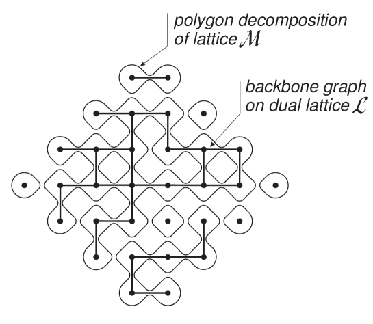
FIG. 6.: Disintegration of the knot diagram on the ${\cal M}$-lattice into ensemble of nonselfintersecting loops (Eulerian circuits) and graph representation of the Potts model on the dual ${\cal L}$-lattice.

(ii) For the given configuration of splittings on ${\cal M}$ and chosen dual lattice ${\cal L}$ let us accept the following convention: we mark the edge of the ${\cal L}$-lattice by the solid line if this edge is not intersected by some polygon on the ${\cal M}$-latice and we leave the corresponding edge unmarked if it is intersected by any polygon—as it is shown in the fig.6. Similarly, the sum $\sum s_{i}b_{i}$ in Eq.(II.37) can be rewritten in terms of marked and unmarked bonds on the ${\cal L}$-lattice

$$\begin{array}[]{ccl}\displaystyle\sum_{i}s_{i}b_{i}&=&\displaystyle\sum_{\rm mark}s_{i}b_{i}+\sum_{\rm nonmark}s_{i}b_{i}\vskip 6.0pt plus 2.0pt minus 2.0pt\\ &=&\displaystyle\sum_{\rm mark}^{\rm horiz}s_{i}b_{i}+\sum_{\rm mark}^{\rm vertic}s_{i}b_{i}+\sum_{\rm nonmark}^{\rm horiz}s_{i}b_{i}+\sum_{\rm nonmark}^{\rm vertic}s_{i}b_{i}\vskip 6.0pt plus 2.0pt minus 2.0pt\\ &=&\displaystyle-\sum_{\rm mark}^{\rm horiz}b_{kl}-\sum_{\rm mark}^{\rm vertic}b_{kl}+\sum_{\rm nonmark}^{\rm horiz}b_{kl}+\sum_{\rm nonmark}^{\rm vertic}b_{kl}\vskip 6.0pt plus 2.0pt minus 2.0pt\\ &=&\displaystyle\sum_{\rm nonmark}b_{kl}-\sum_{\rm mark}b_{kl}=\sum_{\rm all\;edges}b_{kl}-2\sum_{\rm mark}b_{kl}\end{array}$$ (II.38)

where we used the relation $\sum\limits_{\rm nonmark}b_{kl}+\sum\limits_{\rm mark}b_{kl}=\sum\limits_{\rm all\;edges}b_{kl}$.

(iii) Let $m_{s}$ be the number of marked edges and $C_{s}$ be the number of connected components of marked graph. Then the Euler relation reads:

$${\cal S}=2C_{s}+m_{s}-N+\chi$$ (II.39)

The Eq.(II.39) can be proved directly. The $\chi$-value depends on the genus of the surface, which can be covered by the given lattice, (i.e. $\chi$ depends on the boundary conditions). In the thermodynamic limit $N\gg 1$ the $\chi$-dependence should disappear (at least for the flat surfaces), so the standard equality ${\cal S}=2C_{s}+m_{s}-N$ will be assumed below.

By means of definitions (i)-(iii), we can easily convert Eq.(II.37) into the form:

$$\begin{array}[]{c}\displaystyle\left<K\{b_{kl}\}\right>=(A^{2}+A^{-2})^{-(N+1)}\prod_{\mbox{all edges}}^{N}\left[A^{b_{kl}}\right]\\ \displaystyle\hskip 76.82234pt\times\;\sum_{\{G\}}(A^{2}+A^{-2})^{2C_{s}}\prod_{\mbox{mark}}^{m_{s}}\left[A^{-2b_{kl}}(-A^{2}-A^{-2})\right]\end{array}$$ (II.40)

where we used Eq.(II.38) and the fact that $N+1$ is even. Comparing Eq.(II.40) with Eq.(II.25) we immediately conclude that

$$\sum_{\{G\}}(A^{2}+A^{-2})^{2C_{s}}\prod_{\mbox{mark}}^{m_{s}}\left[A^{-2b_{kl}}(-A^{2}-A^{-2})\right]\equiv\sum_{\{{\bf\sigma}\}}\prod_{\{kl\}}\left(1+v_{kl}\delta({\bf\sigma}_{k},{\bf\sigma}_{l})\right)$$ (II.41)

what coincides with the partition function of the Potts system written in the form of dichromatic polynomial. Therefore, we have

$$\begin{array}[]{l}v_{kl}\stackrel{{\scriptstyle def}}{{=}}A^{-2b_{kl}}(-A^{2}-A^{-2})=-1-A^{-4b_{kl}}\vskip 6.0pt plus 2.0pt minus 2.0pt\\ \hskip 8.00003ptq=(A^{2}+A^{-2})^{2}\end{array}$$ (II.42)

Since the “disorder” variables $b_{kl}$ take the discrete values $\pm 1$ only, we get the following expression for the interaction constant $J_{kl}$ (see Eq.(II.26))

$$\frac{J_{kl}}{T}=\ln\left[1-(A^{2}+A^{-2})A^{-2b_{kl}}\right]=\ln[-A^{-4b_{kl}}]$$ (II.43)

Combining Eqs.(II.40)-(II.43) we obtain the following statement.

(a) Take $N$-vertex knot diagram on the lattice ${\cal M}$ with given boundary conditions and fixed set of passages $\{b_{i}\}$. (b) Take the dual lattice ${\cal L}$ in one-to-one correspondence with ${\cal M}$ where one vertex of ${\cal M}$ belongs to one edge of ${\cal L}$.

The Kauffman topological invariant $\left<K(A)\right>$ of regular isotopy for knot diagrams on ${\cal M}$ admits representation in form of 2D Potts system on the dual lattice ${\cal L}$:

$$\left<K(A)\right>=H\bigl{(}A,\{b_{kl}\}\bigr{)}\;Z_{potts}\bigl{[}q(A),\left\{J_{kl}\bigl{(}b_{kl},A\bigr{)}\right\}\bigr{]}$$ (II.44)

where:

$$H\bigl{(}A,\{b_{kl}\}\bigr{)}=\left(A^{2}+A^{-2}\right)^{-(N+1)}\exp\left(\ln A\sum_{\{kl\}}b_{kl}\right)$$ (II.45)

is the trivial multiplier ($H$ does not depend on Potts spins);

$$Z_{potts}\bigl{[}q(A),\left\{J_{kl}\bigl{(}b_{kl},A\bigr{)}\right\}\bigr{]}=\sum_{\{{\bf\sigma}\}}\exp\left\{\sum_{\{kl\}}\frac{J_{kl}\bigl{(}b_{kl},A\bigr{)}}{T}\delta({\bf\sigma}_{k},{\bf\sigma}_{l})\right\}$$ (II.46)

is the Potts partition function with interaction constants, $J_{kl}$, and number of spin states, $q$, defined as follows

$$\frac{J_{kl}}{T}=\ln[-A^{-4b_{kl}}];\qquad q=\left(A^{2}+A^{-2}\right)^{2}$$ (II.47)

and the variables $b_{kl}$ play a role of disorder on edges of the lattice ${\cal L}$ dual to the lattice ${\cal M}$. The connection between $b_{kl}$ and $b_{i}$ is defined by convention

$$b_{kl}=\left\{\begin{array}[]{ll}-b_{i}&\mbox{if $(kl)$-edge is vertical}\vskip 6.0pt plus 2.0pt minus 2.0pt\\ b_{i}&\mbox{if $(kl)$-edge is horizontal}\end{array}\right.$$ (II.48)

Eq.(II.41) has the sense of partition function of the 2D disordered Potts system with the random nearest-neighbor interactions whose distribution remains arbitrary. The set of passages $\{b_{kl}\}$ uniquely determines the actual topological state of the woven carpet for the definite boundary conditions. Therefore the topological problem of the knot invariant determination is reduced to usual statistical problem of calculation of the partition function of the Potts model with the disorder in the interaction constants. Of course, this correspondence is still rather formal because the polynomial variable $A$ is absolutely arbitrary and can take even complex values, but for some regions of $A$ that thermodynamic analogy makes sense and could be useful as we shall see below.

The specific feature of the Potts partition function which gives the representation of the Kauffman algebraic invariant is connected with the existence of the relation between the temperature $T$ and the number of spin states $q$ (see Eq.(II.42)) according to which $T$ and $q$ cannot be considered anymore as independent variables.

2 Algebraic invariants of ambient isotopy

The invariance of the algebraic topological invariant, $f[K]$, with respect to all Reidemeister moves (see Eq.(II.35)) for our system shown in the fig.5 is related to the oriented Eulerian circuits called Hamiltonian walks .

Let us suppose that the orientation of the knot diagram shown in fig.5 is chosen according to the natural orientation of the path representing a knot $K$ in ${\rm{\sf RI\hskip 5.97508pt}}^{3}$. For the defined boundary conditions we get the so-called Manhattan lattice consisting of woven threads with alternating directions.

It follows from the definition of twisting $Tw(K)$ (see the Section 1.3.2) that $Tw(K)$ changes the sign if the direction of one arrow in the vertex is changed to the inverse. Reversing the direction of any arrows in the given vertex even times we return the sign of twisting to the initial value.

We define groups of “even” and “odd” vertices on the lattice ${\cal M}$ as follows. The vertex $i$ is called even (odd) if it belongs to the horizontal (vertical) bond $(kl)$ of the dual lattice ${\cal L}$. Now it is easy to prove that the twisting of the knot on the Manhattan lattice ${\cal M}$ can be written in terms of above defined variables $b_{kl}$. Finally the expression for the algebraic invariant of ambient isotopy $f[K]$ on the lattice ${\cal L}$ reads

$$f[K]=\exp\left(3\ln[-A]\sum_{\{kl\}}b_{kl}\right)\left<K\left(\{b_{kl}\},A\right)\right>$$ (II.49)

where $\left<K\left(\{b_{kl}\},A\right)\right>$ is defined by Eq.(II.44).

E Notion about annealed and quenched realizations of topological disorder

Fixed topological structure of a trajectory of given length fluctuating in space is a typical example of a quenched disorder. Actually, the knot structure is formed during the random closure of the path and cannot be changed without the path rupture. Because of the topological constraints the entire phase space of ensemble of randomly generated closed loops is divided into the separated domains resembling the multi-valley structure of the spin glass phase space. Every domain corresponds to the sub-space of the path configurations with the fixed value of the topological invariant.

The methods of theoretical description of the systems with quenched disorder in interaction constants are rather well developed, especially in regard to the investigation of spin glass models [20]. Central for these methods is the concept of self-averaging which can be explained as follows. Take some additive function $F$ (the free energy, for instance) of some disordered spin system. The function $F$ is the self-averaging quantity if the observed value, $F_{obs}$, of any macroscopic sample of the system coincides with the value $F_{av}$ averaged over the ensemble of disorder realizations:

$$F_{obs}=\left<F\right>_{av}$$

The central technical problem is in calculation of the free energy $F=-T\ln Z$ averaged over the randomly distributed quenched pattern in the interaction constants. In this Section we show that this famous thermodynamic problem of the spin glass physics is closely related to the knot entropy computation.

Another problem arises when averaging the partition function $Z$ (but not the free energy) over the disorder. Such problem is much simpler from computational point of view and corresponds to the case of annealed disorder. Physically such model corresponds to the situation when the topology of the closed loop can be changed. It means that the topological invariant, i.e. the Potts partition function, has to be averaged over all possible realizations of the pattern disorder in the ensemble of open (i.e. unclosed) loops on the lattice. It has been shown in [26] that the calculation of the mean values of topological invariants allows to extract rather rough but nontrivial information about the knot statistics.

1 Entropy of knots. Replica methods

Our main goal is the computation of the probability distribution ${\cal P}_{N}\{f[K]\}$ (see Eq.(II.36)). Although we are unable to evaluate this function exactly, the representation of ${\cal P}_{N}\{f[K]\}$ in terms of disordered Potts system enable us to give an upper estimation for the fraction of randomly generated paths belonging to some definite topological class (in particular, to the trivial one). We use the following chain of inequalities restricting ourselves with the case of regular isotopic knots for simplicity ([24]):

$$\framebox{\parbox{105.2751pt}{Probability ${\cal P}_{N}$ of knot formation in a given topological state}}\leq\framebox{\parbox{147.95424pt}{Probability ${\cal P}_{N}\{K(A)\}$ of knot formation with specific topological invariant $\left<K(A)\right>$ for {\it all} $A$}}\leq\framebox{\parbox{147.95424pt}{Probability ${\cal P}_{N}\{K(A^{*})\}$ of knot formation for {\it specific} va\-lu\-e of $A^{*}$ minimizing the free energy of associated Potts system}}$$ (II.50)

The first inequality is due to the fact that Kauffman invariant of regular isotopic knots is not a complete topological invariant, whereas the last probability in the chain can be written as follows

$${\cal P}_{N}\{K(A^{*})\}=\sum_{\{b_{kl}\}}\Theta\{b_{kl}\}\Delta\Bigl{[}\left<K\{b_{kl},A^{*}\}\right>-\left<K(A^{*})\right>\Bigr{]}$$ (II.51)

where $\sum$ means summation over all possible configurations of the “crossing field” $\{b_{kl}\}$, $\Delta$-function cuts out all states of the field $\{b_{kl}\}$ with specific value of Kauffman invariant $\left<K\{b_{kl},A^{*}\}\right>\equiv\left<K(A^{*})\right>$ and $\Theta\{b_{kl}\}$ is the probability of realization of given crossings configuration.

In principle the distribution $\Theta\{b_{i}\}$ depends on statistics of the path in underlying 3D space and is determined physically by the process of the knot formation. Here we restrict ourselves to the following simplest suppositions:

(i) We regard crossings $\{b_{i}\}$ in different vertices of ${\cal M}$-lattice as completely uncorrelated variables (or, in other words, we assume that the variables $\{b_{kl}\}$ defined on the edges of the ${\cal L}$-lattice are statistically independent):

$$\Theta\{b_{i}\}=\prod_{i}^{N}P(b_{i})$$ (II.52)

(ii) We suppose variable $b_{i}$ (or $b_{kl}$) to take values $\pm 1$ with equal probabilities, i.e.:

$$P(b_{i})=\frac{1}{2}\>\delta(b_{i}-1)+\frac{1}{2}\>\delta(b_{i}+1)$$ (II.53)

The probability of trivial knot formation can be estimated now as follows

$$\begin{array}[]{lll}\displaystyle{\cal P}_{N}^{(0)}(A^{*})&\leq&\displaystyle\sum_{\{b_{kl}\}}\Theta\{b_{kl}\}\Delta\Bigl{[}\ln\left<K\{b_{kl},A^{*}\}\right>\Bigr{]}\vskip 6.0pt plus 2.0pt minus 2.0pt\\ &\simeq&\displaystyle\frac{1}{2\pi}\int_{-\infty}^{\infty}dy\int\ldots\int\prod_{kl}P(b_{kl})db_{kl}\left<K^{iy}\{b_{kl},A^{*}\}\right>\end{array}$$ (II.54)

where $\left<K(A^{*})\right>\equiv 1$ for trivial knots.

Thus our problem is reduced to the calculation of non-integer complex moments of the partition function, i.e., values of the type $\overline{\left<K^{iy}\{b_{kl},A^{*}\}\right>}$. An analogous problem of evaluation of non-integer moments is well known in the spin-glass theory. Indeed, the averaging of the free energy of the system, $\overline{F}$, over quenched random field is widely performed via so-called replica-trick [28]. The idea of the method is as follows. Consider the identity $Z^{n}\equiv e^{n\ln Z}$ and expand the right-hand side up to the first order in $n$. We get $Z^{n}=1+n\ln Z+O(n^{2})$. Now we can write

$$F=-\ln Z=-\lim_{n\to 0}\frac{Z^{n}-1}{n}$$

We proceed with the calculation of the complex moments of the partition function $\left<K\{b_{kl}\}\right>$. In other words we would like to find the averaged value $\overline{\left<K^{n}\right>}$ for integer values of $n$. Then we put $n=iy$ and compute the remaining integral in Eq.(II.54) over $y$-value. Of course, this procedure needs to be verified and it would be of most desire to compare our predictions with the data obtained in numerical simulations. However let us stress that our approach is no more curious than replica one, it would be extremely desirable to test the results obtained by means of computer simulations.

The outline of our calculations is as follows. We begin by rewriting the averaged Kauffman invariant using the standard representation of the replicated Potts partition function and extract the corresponding free energy $\overline{F(A)}$ in the frameworks of the infinite–range mean–field theory in two dimensions. Minimizing $\overline{F(A)}$ with respect to $A$ we find the equilibrium value $A^{*}$. Then we compute the desired probability of trivial knot formation ${\cal P}_{N}^{(0)}(A^{*})$ evaluating the remaining Gaussian integrals.

Averaging the $n$th power of Kauffman invariant over independent values of the “crossing field” $b_{kl}=\pm 1$ we get

$$\begin{array}[]{lll}\displaystyle\overline{\left<K^{n}(A)\right>}&=&\displaystyle\int\ldots\int\prod_{kl}P(b_{kl})db_{kl}K^{2n}\{b_{kl}\}\vskip 6.0pt plus 2.0pt minus 2.0pt\\ &=&\displaystyle\left[2\cosh(2\beta)\right]^{-2n(N+1)}\vskip 6.0pt plus 2.0pt minus 2.0pt\\ &&\displaystyle\times\sum_{\{{\bf\sigma}\}}\prod_{kl}\exp\left\{i\pi\sum_{kl}\delta\bigl{(}{\bf\sigma}_{k}^{\alpha},{\bf\sigma}_{l}^{\alpha}\bigr{)}+\ln\cosh\left[\beta\sum_{\alpha=1}^{n}\Bigl{(}4\delta\bigl{(}{\bf\sigma}_{k}^{\alpha},{\bf\sigma}_{l}^{\alpha}\bigr{)}-1\Bigr{)}\right]\right\}\end{array}$$ (II.55)

where $\beta=\ln A$. Let us break for a moment the connection between the number of spin states, $q$, and interaction constant and suppose $|\beta|\ll 1$. Later on we shall verify the selfconsistency of this approximation. Now the exponent in the last expression can be expanded as a power series in $\beta$. Keeping the terms of order $\beta^{2}$ only, we rewrite Eq.(II.55) in the standard form of $n$-replica Potts partition function

$$\begin{array}[]{l}\displaystyle\overline{\left<K^{n}(A)\right>}=\left[2\cosh(2\beta)\right]^{-2n(N+1)}\exp\left[N\left(\frac{1}{2}\beta^{2}n^{2}\right)\right]\vskip 6.0pt plus 2.0pt minus 2.0pt\\ \displaystyle\times\sum_{\{{\bf\sigma}_{1}\ldots{\bf\sigma}_{n}\}}\exp\Biggl{\{}\frac{J^{2}}{2}\sum_{kl}^{N}\sum_{\alpha\neq\beta}^{n}{\bf\sigma}_{ka}^{\alpha}{\bf\sigma}_{kb}^{\beta}{\bf\sigma}_{la}^{\alpha}{\bf\sigma}_{lb}^{\beta}+\left(\frac{J^{2}}{2}(q-2)+\bar{J}_{0}\right)\sum_{kl}^{N}\sum_{\alpha=1}^{n}{\bf\sigma}_{ka}^{\alpha}{\bf\sigma}_{lb}^{\beta}\Biggr{\}}\end{array}$$ (II.56)

where spin indexes $a,b$ change in the interval $[0,q-1]$, $\beta^{2}\ll 1$ and

$$\begin{array}[]{rll}J^{2}&=&16\beta^{2}\vskip 6.0pt plus 2.0pt minus 2.0pt\\ \bar{J}_{0}&=&i\pi-4\beta^{2}n\vskip 6.0pt plus 2.0pt minus 2.0pt\\ q&=&4+16\beta^{2}>4\end{array}$$ (II.57)

According to the results of Cwilich and Kirkpatrick [29] and later works (see, for instance, [30]), the spin-glass ordering takes place and the usual ferromagnetic phase makes no essential contribution to the free energy under the condition

$$\frac{\bar{J}_{0}}{J}<\frac{q-4}{2}$$ (II.58)

Substituting Eq.(II.57) into Eq.(II.58) it can be seen that $\Re(\mbox{l.h.s.})<\Re(\mbox{r.h.s})$ in Eq.(II.58) for all $\beta$. Thus, we expect that the spin-glass ordering (in the infinite-range model) corresponds to the solutions

$$\begin{array}[]{lll}\displaystyle m_{a}^{\alpha}&=&\displaystyle\Bigl{<}q\delta({\bf\sigma}_{k}^{\alpha},a)-1\Bigr{>}=0\vskip 6.0pt plus 2.0pt minus 2.0pt\\ \displaystyle Q_{ab}^{\alpha\beta}&=&\displaystyle\Bigl{<}q\delta({\bf\sigma}_{k}^{\alpha},a)-1\Bigr{>}\Bigl{<}q\delta({\bf\sigma}_{k}^{\beta},b)-1\Bigr{>}\neq 0\end{array}$$

where $m_{a}^{\alpha}$ and $Q_{ab}^{\alpha\beta}$ are the ferromagnetic and spin-glass order parameters respectively. If it is so, we can keep the term in the exponent (Eq.(II.56)) corresponding to inter-replica interactions only.

We follow now the standard scheme of analysis of Potts spin glasses partition function exhaustively described in [29, 31, 30]; main steps of this analysis are shortly represented below. Performing the Hubbard-Stratonovich transformation to the scalar fields $Q^{\alpha\beta}_{iab}$ and implying the homogeneous isotropic solution of the form $Q^{\alpha\beta}_{iab}=Q^{\alpha\beta}_{i}\delta_{ab}$, we can write down the value $\overline{\left<K^{n}\right>}$ (Eq.(II.56)) as follows ([29]):

$$\begin{array}[]{c}\displaystyle\overline{\left<K^{n}\right>}=\exp\Biggl{\{}N\Biggl{[}\ln\frac{\pi}{J^{2}}n(n-1)(q-1)^{2}-\ln\left(2\cosh{J\over 2}\right)+\frac{J^{2}n^{2}}{32}\Biggr{]}\Biggr{\}}\vskip 6.0pt plus 2.0pt minus 2.0pt\\ \displaystyle\times\sum_{\{{\bf\sigma}\}}\int\prod_{i}dQ_{i}^{\alpha\beta}\exp\left\{-\int H\{Q_{i}^{\alpha\beta}\}d^{2}x\right\}\end{array}$$ (II.59)

where

$$\begin{array}[]{l}\displaystyle H\{Q^{\alpha\beta}\}=(q-1)\Biggl{[}{1\over 4}\left(\frac{2}{J^{2}}-1\right)\sum_{\alpha\neq\beta}(Q^{\alpha\beta})^{2}-{1\over 6}\sum_{\alpha\neq\beta\neq\gamma}Q^{\alpha\beta}Q^{\beta\gamma}Q^{\gamma\alpha}\vskip 6.0pt plus 2.0pt minus 2.0pt\\ \displaystyle\hskip 56.9055pt-{{q-2}\over{12}}\sum_{\alpha\neq\beta}(Q^{\alpha\beta})^{3}-{{q-2}\over 4}\sum_{\alpha\neq\beta\neq\gamma}(Q^{\alpha\beta})^{2}Q^{\beta\gamma}Q^{\gamma\alpha}\vskip 6.0pt plus 2.0pt minus 2.0pt\\ \displaystyle\hskip 56.9055pt-{1\over 8}\sum_{\alpha\neq\beta\neq\gamma\neq\delta}Q^{\alpha\beta}Q^{\beta\gamma}Q^{\gamma\delta}Q^{\delta\alpha}-{{q^{2}-6q+6}\over{48}}\sum_{\alpha\beta}(Q^{\alpha\beta})^{4}\Biggr{]}\end{array}$$ (II.60)

In [31, 29] it was shown, that the mean-field replica symmetric solution of the mean-field Potts spin glass is unstable for $q\geq 2$ and the right ansatz of Eqs.(II.59)-(II.60) corresponds to the first level of Parisi replica breaking scheme for spin glasses. Hence, we have

$$Q^{\alpha\beta}=\left\{\begin{array}[]{ll}Q&\mbox{if $\alpha$ and $\beta$ belong to the same group of $m$ replicas}\vskip 6.0pt plus 2.0pt minus 2.0pt\\ 0&\mbox{otherwise}\end{array}\right.$$ (II.61)

Analysis shows that for $q>4$ (our case) the transition to the glassy state corresponds to $m=1$ which implies the accessory condition $F_{pm}=F_{sg}$, where $F_{pm}$ and $F_{sg}$ are the free energies of paramagnetic and spin-glass phases respectively. The transition occurs at the point

$$1-{2\over{J^{2}}}={{(q-4)^{2}}\over{3(q^{2}-18q+42)}}$$ (II.62)

Substituting Eq.(II.57) into Eq.(II.62) we find the self-consistent value of reverse temperature of a spin-glass transition, $\beta_{tr}$:

$$\beta_{tr}\approx 0.35$$ (II.63)

This numerical value is consistent with the condition $\beta^{2}_{tr}\ll 1$ implied above in the course of expansion of Eq.(II.56).

According to the results of the work [29] the $n$-replica free energy near the transition point has the following form

$$F\simeq\frac{1}{64}Nn(q-1)^{2}Q_{tr}\left(\frac{1}{\beta^{2}}-\frac{1}{\beta^{2}_{tr}}\right)^{2}$$ (II.64)

with the following expression of the spin-glass order parameter

$$Q_{tr}=\frac{2(4-q)}{q^{2}-18q+42}>0$$ (II.65)

From Eq.(II.64) we conclude that the free energy $\overline{F}$ reaches its minimum as a function of $A=\exp{(\beta)}$ just at the point $A^{*}=\exp(\beta_{tr})$. Using Eqs.(II.64) and (II.65) we rewrite the expression for the averaged $n$-replica Kauffman invariant $\overline{\left<K^{n}\right>}$ in the vicinity of $\beta_{tr}$ as follows (compare to [29]):

$$\begin{array}[]{l}\displaystyle\overline{\left<K^{2n}\right>}\simeq\exp\Biggl{\{}Nn^{2}\Biggl{[}\left(3+16\beta^{2}\right)^{2}\ln\frac{\pi}{16\beta^{2}}+\frac{\beta^{2}}{2}\Biggr{]}-\vskip 6.0pt plus 2.0pt minus 2.0pt\\ \displaystyle\hskip 28.45274ptNn\Biggl{[}\left(3+16\beta^{2}\right)^{2}\ln\frac{\pi}{16\beta^{2}}+\ln 2+\frac{\beta^{2}}{2}-\frac{\left(3+16\beta^{2}\right)^{2}\left(\beta^{-2}-\beta_{tr}^{-2}\right)^{2}\beta_{tr}^{2}}{\left(4+16\beta_{tr}^{2}\right)^{2}-18\left(4+16\beta_{tr}^{2}\right)+42}\Biggr{]}\Biggr{\}}\end{array}$$ (II.66)

Substituting Eq.(II.66) into Eq.(II.54) and bearing in mind, that $n=iy$, we can easily evaluate the remaining Gaussian integral over $y$-value and obtain the result for ${\cal P}^{(0)}_{N}(A)$. As it has been mentioned above, to get the simplest estimation for probability of trivial knot formation, we use the last inequality in the chain of equations (II.50) corresponding to the choice $A=A^{*}\equiv\exp(\beta_{tr})$:

$${\cal P}^{(0)}_{N}(A^{*})\simeq\exp(c\,N);\qquad c\approx 1$$ (II.67)

This dependence it is not surprising from the point of view of statistical mechanics because the value $\eta={\cal P}^{(0)}_{N}(A^{*})$ is proportional to the free energy of the Potts system. But from the topological point of view the value $\eta$ has the sense of typical “complexity’ of the knot (see also Section 3). The fact that $\eta$ grows linearly with $N$ means that the maximum of the distribution function $P(\eta,N)$ is in the region of very “complex” knots, i.e. knots far from trivial. This circumstance directly follows from the non-commutative nature of topological interactions.

III Random walks on locally non-commutative groups

Recent years have been marked by the emergence of more and more problems related to the consideration of physical processes on non-commutative groups. In trying to classify such problems, we distinguish between the following categories in which the non-commutative origin of phenomena appear with perfect clarity:

1. Problems connected with the spectral properties of the Harper–Hofstadter equation [14] dealing with the electron dynamics on the lattice in a constant magnetic field. We mean primarily the consideration of groups of magnetic translations and properties of quantum planes [32, 15].

2. Problems of classical and quantum chaos on hyperbolic manifolds: spectral properties of dynamical systems and derivation of trace formulae [33, 34, 35] as well as construction of probability measures for random walks on modular groups [36].

3. Problems giving rise to application of quantum group theory in physics: deformations of classical abelian objects such as harmonic oscillators [4] and standard random walks [3].

4. Problems of knot theory and statistical topology: construction of nonabelian topological invariants [5, 23], consideration of probabilistic behavior of the words on the simplest non-commutative groups related to topology (such as braid groups) [37], statistical properties of ”anyonic” systems [38].

5. Classical problems of random matrix and random operator theory and localization phenomena: determination of Lyapunov exponents for products of random non-commutative matrices [39, 40, 41], study of the spectral properties and calculation of the density of states of large random matrices [21, 42].

Certainly, such a division of problems into these categories is very speculative and reflects to a marked degree the authors’ personal point of view. However, we believe that the enumerated items reflect, at least partially, the currently growing interest in theoretical physics of the ideas of non-commutative analysis. Let us stress that we do not touch upon the pure mathematical aspects of non-commutative analysis in this paper and the problems discussed in the present work mainly concern the points 4 and 5 of the list above.

In the present Section we continue analyzing the statistical problems in knot theory, but our attention is paid to some more delicate matters related to investigation of correlations in knotted random paths caused by the topological constraints. The methods elaborated in Section 2 allow us to discuss these questions but we find it more reasonable to take a look at the problems of knot entropy estimation in terms of conventional random matrix theory. We believe that many non-trivial properties of the knot entropy problem can be clearly explained in context of the limit behavior of random walks over the elements of some non-commutative (hyperbolic) groups [46].

Another reason which forces us to consider the limit distributions (and conditional limit distributions) of Markov chains on locally non-commutative discrete groups is due to the fact that this class of problems could be regarded as the first step in a consistent harmonic analysis on the multiconnected manifolds (like Teichmüller space); see also the Section 4.

A Brownian bridges on simplest non-commutative groups and knot statistics

As it follows from the said above the problems dealing with the investigation of the limit distributions of random walks on non-commutative groups is not a new subject in the probability theory and statistical physics.

However in the context of “topologically-probabilistic” consideration the problems dealing with distributions of non-commutative random walks are practically out of discussion, except for very few special cases [41, 49, 43]. Particularly, in these works it has been shown that statistics of random walks with the fixed topological state with respect to the regular array of obstacles on the plane can be obtained from the limit distribution of the so-called “Brownian bridges” (see the definition below) on the universal covering—the graph with the topology of Cayley tree. The analytic construction of nonabelian topological invariant for the trajectories on the double punctured plane and statistics of simplest nontrivial random braid $B_{3}$ was shortly discussed in [44].

Below we calculate the conditional limit distributions of the Brownian bridges on the braid group $B_{3}$ and derive the limit distribution of powers of Alexander polynomial of knots generated by random $B_{3}$-braids. We also discuss the limit distribution of random walks on locally free groups and express some conjectures about statistics of random walks on the group $B_{n}$. More extended discussion of the results concerning the statistics of Markov chains on the braid and locally free groups one can find in [52, 53, 54].

1 Basic definitions and statistical model

The braid group $B_{n}$ of $n$ strings has $n-1$ generators $\{\sigma_{1},\sigma_{2},\ldots,\sigma_{n-1}\}$ with the following relations:

$$\begin{array}[]{ll}\vskip 6.0pt plus 2.0pt minus 2.0pt\sigma_{i}\sigma_{i+1}\sigma_{i}=\sigma_{i+1}\sigma_{i}\sigma_{i+1}&\qquad(1\leq i<n-1)\\ \sigma_{i}\sigma_{j}=\sigma_{j}\sigma_{i}&\qquad(|i-j|\geq 2)\vskip 6.0pt plus 2.0pt minus 2.0pt\\ \sigma_{i}\sigma_{i}^{-1}=\sigma_{i}^{-1}\sigma_{i}=e&\end{array}$$ (III.1)

Any arbitrary word written in terms of “letters”—generators from the set $\{\sigma_{1},\ldots,\break\sigma_{n-1},\sigma_{1}^{-1},\ldots,\sigma_{n-1}^{-1}\}$—gives a particular braid. The geometrical interpretation of braid generators is shown below:

The length of the braid is the total number of the used letters, while the minimal irreducible length hereafter referred to as the “primitive word” is the shortest noncontractible length of a particular braid which remains after applying all possible group relations Eq.(III.1). Diagrammatically the braid can be represented as a set of crossed strings going from the top to the bottom appeared after subsequent gluing the braid generators.

The closed braid appears after gluing the “upper” and the “lower” free ends of the braid on the cylinder.

Any braid corresponds to some knot or link. So, it is feasible principal possibility to use the braid group representation for the construction of topological invariants of knots and links. However the correspondence between braids and knots is not mutually single valued and each knot or link can be represented by infinite series of different braids. This fact should be taken into account in course of knot invariant construction.

Take a knot diagram $K$ in general position on the plane. Let $f[K]$ be the topological invariant of the knot $K$. One of the ways to construct the knot invariant using the braid group representation is as follows.

1. Represent the knot by some braid $b\in B_{n}$. Take the function $f$

$$f:\;B_{n}\to{\sf C}$$

Demand $f$ to take the same value for all braids $b$ representing the given knot $K$. That condition is established in the well-known Markov-Birman theorem (see, for instance, [55]):

The function $f_{K}\{b\}$ defined on the braid $b\in B_{n}$ is the topological invariant of a knot or link if and only if it satisfies the following “Markov condition”:

$$\begin{array}[]{lc}\vskip 6.0pt plus 2.0pt minus 2.0ptf_{K}\{b^{\prime}\,b^{\prime\prime}\}=f_{K}\{b^{\prime\prime}\,b^{\prime}\}&\\ f_{K}\{b^{\prime}\,\sigma_{n}\}=f_{K}\{\sigma_{n}\,b^{\prime}\}=f_{K}\{b^{\prime}\}&\quad b^{\prime},b^{\prime\prime}\in B_{n}\end{array}$$ (III.2)

where $b^{\prime}$ and $b^{\prime\prime}$ are two subsequent sub-words in the braid — see fig.7.

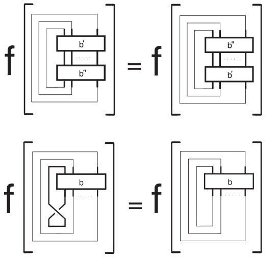
FIG. 7.: Geometric representation of Eqs.(III.2).

2. Now the invariant $f_{K}\{b\}$ can be constructed using the linear functional $\varphi\{b\}$ defined on the braid group and called Markov trace. It has the following properties

$$\begin{array}[]{l}\varphi\{b^{\prime}\,b^{\prime\prime}\}=\varphi\{b^{\prime\prime}\,b^{\prime}\}\vskip 6.0pt plus 2.0pt minus 2.0pt\\ \varphi\{b^{\prime}\,\sigma_{n}\}=\tau\varphi\{b^{\prime}\}\vskip 6.0pt plus 2.0pt minus 2.0pt\\ \varphi\{b^{\prime}\,\sigma_{n}^{-1}\}=\bar{\tau}\varphi\{b^{\prime}\}\end{array}$$ (III.3)

where

$$\tau=\varphi\{\sigma_{i}\},\quad\bar{\tau}=\varphi\{\sigma_{i}^{-1}\};\qquad i\in[1,n-1]$$ (III.4)

The invariant $f_{K}\{b\}$ of the knot $K$ is connected with the linear functional $\varphi\{b\}$ defined on the braid $b$ as follows

$$f_{K}\{b\}=(\tau\bar{\tau})^{-(n-1)/2}\left(\frac{\bar{\tau}}{\tau}\right)^{\frac{1}{2}\bigl{(}\#(+)-\#(-)\bigr{)}}\varphi\{b\}$$ (III.5)

where $\#(+)$ and $\#(-)$ are the numbers of “positive” and “negative” crossings in the given braid correspondingly.

The Alexander algebraic polynomials are the first well-known invariants of such type. In the beginning of 1980s Jones discovered the new knot invariants. He used the braid representation “passed through” the Hecke algebra relations, where the Hecke algebra, $H_{n}(t)$, for $B_{n}$ satisfies both braid group relations Eq.(III.1) and an additional “reduction” relation (see the works [55, 56])

$$\sigma_{i}^{2}=(1-t)\sigma_{i}+t$$ (III.6)

Now the trace $\varphi\{b\}=\varphi(t)\{b\}$ can be said to take the value in the ring of polynomials of one complex variable $t$. Consider the functional $\varphi(t)$ over the braid $\{b^{\prime}\,\sigma_{i}\,b^{\prime\prime}\}$. Eq.(III.6) allows us to get the recursion (skein) relations for $\varphi(t)$ and for the invariant $f_{K}(t)$ (see for details [58]):

$$\varphi(t)\{b^{\prime}\sigma_{i}b^{\prime\prime}\}=(1-t)\varphi(t)\{b^{\prime}b^{\prime\prime}\}+t\varphi(t)\{b^{\prime}\sigma_{i}^{-1}b^{\prime\prime}\}$$ (III.7)

and

$$f_{K}^{+}(t)-t\left(\frac{\bar{\tau}}{\tau}\right)f_{K}^{-}(t)=(1-t)\left(\frac{\bar{\tau}}{\tau}\right)^{1/2}f_{K}^{0}(t)$$ (III.8)

where $f_{K}^{+}\equiv f\{b^{\prime}\,\sigma_{i}\,b^{\prime\prime}\}$;  $f_{K}^{-}\equiv f\{b^{\prime}\,\sigma_{i}^{-1}\,b^{\prime\prime}\}$;  $f_{K}^{0}\equiv f\{b^{\prime}\,b^{\prime\prime}\}$ and the fraction $\displaystyle\frac{\bar{\tau}}{\tau}$ depends on the used representation.

3. The tensor representations of the braid generators can be written as follows

$$\sigma_{i}(u)=\lim_{u\to\infty}\sum_{klmn}R^{km}_{ln}(u)I^{(1)}\otimes\cdots I^{(i-1)}\otimes E_{nk}^{i}\otimes E_{ml}^{i+1}\otimes I^{(i+1)}\otimes\cdots I^{(n)}$$ (III.9)

where $I^{(i)}$ is the identity matrix acting in the position $i$; $E_{nk}$ is a matrix with $(E_{nk})_{pq}=\delta_{np}\delta_{kq}$ and $R^{km}_{ln}$ is the matrix satisfying the Yang-Baxter equation

$$\sum_{abc}R^{bq}_{cr}(v)R^{ap}_{kc}(u+v)R^{ia}_{jb}(u)=\sum_{abc}R^{ap}_{bq}(u)R^{ia}_{cr}(u+v)R^{jb}_{ka}(v)$$ (III.10)

In that scheme both known polynomial invariants (Jones and Alexander) ought to be considered. In particular, it has been discovered in [57, 58] that the solutions of Eq.(III.10) associated with the groups $SU_{q}(2)$ and $GL(1,1)$ are linked to Jones and Alexander invariants correspondingly. To be more specific:

(a) $\displaystyle\frac{\bar{\tau}}{\tau}=t^{2}$ for Jones invariants, $f_{K}(t)\equiv V(t)$. The corresponding skein relations are

$$t^{-1}V^{+}(t)-tV^{-}(t)=(t^{-1/2}-t^{1/2})V^{0}(t)$$ (III.11)

and

(b) $\displaystyle\frac{\bar{\tau}}{\tau}=t^{-1}$ for Alexander invariants, $f_{K}(t)\equiv\nabla(t)$. The corresponding skein relations  are

$$\nabla^{+}(t)-\nabla^{-}(t)=(t^{-1/2}-t^{1/2})\nabla^{0}(t)$$ (III.12)

To complete this brief review of construction of polynomial invariants from the representation of the braid groups it should be mentioned that the Alexander invariants allow also another useful description [59]. Write the generators of the braid group in the so-called Magnus representation

$$\sigma_{j}\equiv\hat{\sigma}_{j}=\left(\begin{array}[]{ccccccccc}1&0&\cdots&&\\ 0&\ddots&&&\\ \vdots&&\framebox{A}&&\vdots\\ &&&\ddots&0\\ &&\cdots&0&1\end{array}\right)\leftarrow j\mbox{th row};\;A=\left(\begin{array}[]{ccc}1&0&0\\ t&-t&1\\ 0&0&1\end{array}\right)$$ (III.13)

Now the Alexander polynomial of the knot represented by the closed braid $W=\prod_{j=1}^{N}\sigma_{{\alpha}_{j}}$ of the length $N$ one can write as follows

$$(1+t+t^{2}+\ldots+t^{n-1})\,\nabla(t)\{A\}=\det\left[\prod_{j=1}^{N}\hat{\sigma}_{{\alpha}_{j}}-e\right]$$ (III.14)

where index $j$ runs “along the braid”, i.e. labels the number of used generators, while the index $\alpha=\{1,\ldots,n-1,n,\dots,2n-2\}$ marks the set of braid generators (letters) ordered as follows $\{\sigma_{1},\ldots,\sigma_{n-1},\sigma_{1}^{-1},\ldots,\sigma_{n-1}^{-1}\}$. In our further investigations we repeatedly address to that representation.

We are interested in the limit behavior of the knot or link invariants when the length of the corresponding braid tends to infinity, i.e. when the braid “grows”. In this case we can rigorously define some topological characteristics, simpler than the algebraic invariant, which we call the knot complexity.

Call the knot complexity, $\eta$, the power of some algebraic invariant, $f_{K}(t)$ (Alexander, Jones, HOMFLY) (see also [26])

$$\eta=\lim_{|t|\rightarrow\infty}\frac{\ln f_{K}(t)}{\ln|t|}$$ (III.15)

Remark. By definition, the “knot complexity” takes one and the same value for rather broad class of topologically different knots corresponding to algebraic invariants of one and the same power, being from this point of view weaker topological characteristics than complete algebraic polynomial. Let us summarize the advantages of knot complexity.

(i) One and the same value of $\eta$ characterizes a narrow class of “topologically similar” knots which is, however, much broader than the class represented by the polynomial invariant $X(t)$. This enables us to introduce the smoothed measures and distribution functions for $\eta$.

(ii) The knot complexity $\eta$ describes correctly (at least from the physical point of view) the limit cases: $\eta=0$ corresponds to “weakly entangled” trajectories whereas $\eta\sim N$ matches the system of “strongly entangled” paths.

(iii) The knot complexity keeps all nonabelian properties of the polynomial invariants.

(iv) The polynomial invariant can give exhaustive information about the knot topology. However when dealing with statistics of randomly generated knots, we frequently look for rougher characteristics of “topologically different” knots. A similar problem arises in statistical mechanics when passing from the microcanonical ensemble to the Gibbs one: we lose some information about details of particular realization of the system but acquire smoothness of the measure and are able to apply standard thermodynamic methods to the system in question.

The main purpose of the present section is the estimation of the limit probability distribution of $\eta$ for the knots obtained by randomly generated closed $B_{n}$-braids of the length $N$. It should be emphasized that we essentially simplify the general problem “of knot entropy”. Namely, we introduce an additional requirement that the knot should be represented by a braid from the group $B_{n}$ without fail.

We begin the investigation of the probability properties of algebraic knot invariants by analyzing statistics of the random loops (“Brownian bridges”) on simplest non-commutative groups. Most generally the problem can be formulated as follows. Take the discrete group ${\cal G}_{n}$ with a fixed finite number of generators $\{g_{1},\ldots,g_{n-1}\}$. Let $\nu$ be the uniform distribution on the set $\{g_{1},\ldots,g_{n-1},g_{1}^{-1},\ldots,g_{n-1}^{-1}\}$. For convenience we suppose $h_{j}=g_{i}$ for $j=i$ and $h_{j}=g_{i}^{-1}$ for $j=i+n-1$; $\nu(h_{j})=\frac{1}{2n-2}$ for any $j$. We construct the (right-hand) side random walk (the random word) on ${\cal G}_{n}$ with a transition measure $\nu$, i.e. the Markov chain $\{\xi_{n}\}$, $\xi_{0}=e\in{\cal G}_{n}$ and Prob$(\xi_{j}=u|\xi_{j-1}=v)=\nu(v^{-1}u)=\frac{1}{2n-2}$. It means that with the probability $\frac{1}{2n-2}$ we add the element $h_{\alpha_{N}}$ to the given word $h_{N-1}=h_{\alpha_{1}}h_{\alpha_{2}}\ldots h_{\alpha_{N-1}}$ from the right-hand side .

The random word $W$ formed by $N$ letters taken independently with the uniform probability distribution $\nu=\frac{1}{2n-2}$ from the set $\{g_{1},\ldots,$ $g_{n-1},g_{1}^{-1},\ldots,g_{n-1}^{-1}\}$ is called the Brownian bridge (BB) of length $N$ on the group ${\cal G}_{n}$ if the shortest (primitive) word of $W$ is identical to the unity.

Two questions require most of our attention:

1. What is the probability distribution $P(N)$ of the Brownian bridge on the group ${\cal G}_{n}$.

2. What is the conditional probability distribution $P(k,m|N)$ of the fact that the sub-word $W^{\prime}$ consisting of first $m$ letters of the $N$–letter word $W$ has the primitive path $k$ under the condition that the whole word $W$ is the Brownian bridge on the group ${\cal G}_{n}$. (Hereafter $P(k,m|N)$ is referred to as the conditional distribution for BB.)

It has been shown in the paper [41] that for the free group the corresponding problem can be mapped on the investigation of the random walks on the simply connected tree. Below we represent shortly some results concerning the limit behavior of the conditional probability distribution of BB on the Cayley tree. In the case of braids the more complicated group structure does not allow us to apply the same simple geometrical image directly. Nevertheless the problem of the limit distribution for the random walks on $B_{n}$ can be reduced to the consideration of the random walk on some graph $C(\Gamma)$. In case of the group $B_{3}$ we are able to construct this graph evidently, whereas for the group $B_{n}$ ($n\geq 4$) we give upper estimations for the limit distribution of the random walks considering the statistics of Markov chains on so-called local groups.

2 Random process on $PSL(2,{\rm{\sf ZZ\hskip 1.70717pt}})$, $B_{3}$ and limit distribution of powers of Alexander invariant

We begin with computing the distribution function for the conditional random process on the simplest nontrivial braid group $B_{3}$. The group $B_{3}$ can be represented by $2\times 2$ matrices. To be specific, the braid generators $\sigma_{1}$ and $\sigma_{2}$ in the Magnus representation [59] look as follows:

$$\sigma_{1}=\left(\begin{array}[]{cc}-t&1\\ 0&1\end{array}\right);\qquad\sigma_{2}=\left(\begin{array}[]{cc}1&0\\ t&-t\end{array}\right),$$ (III.16)

where $t$ is “the spectral parameter”. It is well known that for $t=-1$ the matrices $\sigma_{1}$ and $\sigma_{2}$ generate the group $PSL(2,\rm{\sf ZZ\hskip 1.70717pt})$ in such a way that the whole group $B_{3}$ is its central extension with the center

$$(\sigma_{1}\sigma_{2}\sigma_{1})^{4\lambda}=(\sigma_{2}\sigma_{1}\sigma_{2})^{4\lambda}=(\sigma_{1}\sigma_{2})^{6\lambda}=(\sigma_{2}\sigma_{1})^{6\lambda}=\left(\begin{array}[]{cc}t^{6\lambda}&0\\ 0&t^{6\lambda}\end{array}\right)$$ (III.17)

First restrict ourselves with the examination of the group $PSL(2,\rm{\sf ZZ\hskip 1.70717pt})$, for which we define $\tilde{\sigma}_{1}=\sigma_{1}$ and $\tilde{\sigma}_{2}=\sigma_{2}$ (at $t=-1$).

The canonical representation of $PSL(2,\rm{\sf ZZ\hskip 1.70717pt})$ is given by the unimodular matrices $S,T$:

$$S=\left(\begin{array}[]{cc}0&1\\ -1&0\end{array}\right);\qquad T=\left(\begin{array}[]{cc}1&1\\ 0&1\end{array}\right)$$ (III.18)

The braiding relation $\tilde{\sigma}_{1}\tilde{\sigma}_{2}\tilde{\sigma}_{1}=\tilde{\sigma}_{2}\tilde{\sigma}_{1}\tilde{\sigma}_{2}$ in the $\{S,T\}$-representation takes the form

$$S^{2}TS^{-2}T^{-1}=1$$ (III.19)

in addition we have

$$S^{4}=(ST)^{3}=1$$ (III.20)

This representation is well known and signifies the fact that in terms of $\{S,T\}$-generators the group $SL(2,\rm{\sf ZZ\hskip 1.70717pt})$ is a free product $Z^{2}\otimes Z^{3}$ of two cyclic groups of the 2nd and the 3rd orders correspondingly.

The connection of $\{S,T\}$ and $\{\tilde{\sigma}_{1},\tilde{\sigma}_{2}\}$ is as follows

$$\begin{array}[]{ll}\tilde{\sigma}_{1}=T&(T=\tilde{\sigma}_{1})\vskip 6.0pt plus 2.0pt minus 2.0pt\\ \tilde{\sigma}_{2}=T^{-1}ST^{-1}&(S=\tilde{\sigma}_{1}\tilde{\sigma}_{2}\tilde{\sigma}_{1})\end{array}$$ (III.21)

The modular group $PSL(2,\rm{\sf ZZ\hskip 1.70717pt})$ is a discrete subgroup of the group $PSL(2,\rm{\sf RI\hskip 5.97508pt})$. The fundamental domain of $PSL(2,\rm{\sf ZZ\hskip 1.70717pt})$ has the form of a circular triangle $ABC$ with angles $\left\{0,\frac{\pi}{3},\frac{\pi}{3}\right\}$ situated in the upper half-plane Im$\zeta>0$ of the complex plane $\zeta=\xi+i\eta$ (see fig.8 for details). According to the definition of the fundamental domain, at least one element of each orbit of $PSL(2,\rm{\sf ZZ\hskip 1.70717pt})$ lies inside $ABC$-domain and two elements lie on the same orbit if and only if they belong to the boundary of the $ABC$-domain. The group $PSL(2,\rm{\sf ZZ\hskip 1.70717pt})$ is completely defined by its basic substitutions under the action of generators $S$ and $T$:

$$\begin{array}[]{l}S:\quad\zeta\to-1/\zeta\vskip 6.0pt plus 2.0pt minus 2.0pt\\ T:\quad\zeta\to\zeta+1\end{array}$$ (III.22)

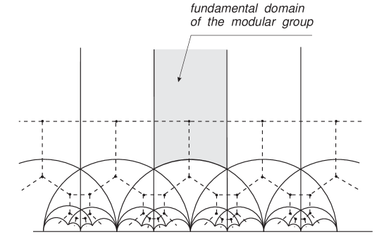
FIG. 8.: The Riemann surface for the modular group The graph $C(\Gamma)$ representing the topological structure of $PSL(2,~{}\rm{\sf ZZ\hskip 1.70717pt})$ is shown by the dashed line.

Let us choose an arbitrary element $\zeta_{0}$ from the fundamental domain and construct a corresponding orbit. In other words, we raise a graph, $C(\Gamma)$, which connects the neighboring images of the initial element $\zeta_{0}$ obtained under successive action of the generators from the set $\{S,T,S^{-1},T^{-1}\}$ to the element $\zeta_{0}$. The corresponding graph is shown in the fig.8 by the broken line and its topological structure is clearly reproduced in fig.9. It can be seen that although the graph $C(\Gamma)$ does not correspond to the free group and has local cycles, its “backbone”, $C(\gamma)$, has Cayley tree structure but with the reduced number of branches as compared to the free group $C(\Gamma_{2})$.

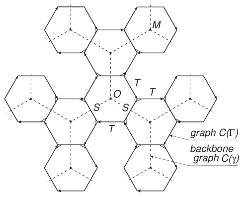
FIG. 9.: The graph $C(\Gamma)$ and its backbone graph $C(\gamma)$ (see the explanations in the text).

Turn to the problem of limit distribution of a random walk on the graph $C(\Gamma)$. The walk is determined as follows:

1. Take an initial point (“root”) of the random walk on the graph $C(\Gamma)$. Consider the discrete random jumps over the neighboring vertices of the graph with the transition probabilities induced by the uniform distribution $\nu$ on the set of generators $\{\tilde{\sigma}_{1},\tilde{\sigma}_{2},\tilde{\sigma}_{1}^{-1},\tilde{\sigma}_{2}^{-1}\}$. These probabilities are (see Eq.(III.21))

$$\begin{array}[]{l}\vskip 6.0pt plus 2.0pt minus 2.0pt\mbox{Prob}(\xi_{n}=T\zeta_{0}\;|\;\xi_{n-1}=\zeta_{0})=\frac{1}{4}\\ \vskip 6.0pt plus 2.0pt minus 2.0pt\mbox{Prob}(\xi_{n}=(T^{-1}ST^{-1})\zeta_{0}\;|\;\xi_{n-1}=\zeta_{0})=\frac{1}{4}\\ \vskip 6.0pt plus 2.0pt minus 2.0pt\mbox{Prob}(\xi_{n}=T^{-1}\zeta_{0}\;|\;\xi_{n-1}=\zeta_{0})=\frac{1}{4}\\ \vskip 6.0pt plus 2.0pt minus 2.0pt\mbox{Prob}(\xi_{n}=(TS^{-1}T)\zeta_{0}\;|\;\xi_{n-1}=\zeta_{0})=\frac{1}{4}\end{array}$$ (III.23)

The following facts should be taken into account: the elements $S\zeta_{0}$ and $S^{-1}\zeta_{0}$ represent one and the same point, i.e. coincide (as it follows from Eq.(III.22)); the process is Markovian in terms of the alphabet $\{\tilde{\sigma}_{1},\ldots,\tilde{\sigma}_{2}^{-1}\}$ only; the total transition probability is conserved.

2. Define the shortest distance, $k$, along the graph between the root and terminal points of the random walk. According to its construction, this distance coincides with the length $|W_{\{S,T\}}|$ of the minimal irreducible word $W_{\{S,T\}}$ written in the alphabet $\{S,T,S^{-1},T^{-1}\}$. The link of the distance, $k$, with the length $|W_{\{\tilde{\sigma}_{1},\tilde{\sigma}_{2}\}}|$ of the minimal irreducible word $W_{\{\tilde{\sigma}_{1},\tilde{\sigma}_{2}\}}$ written in terms of the alphabet $\{\tilde{\sigma}_{1},\tilde{\sigma}_{2},\tilde{\sigma}_{1}^{-1},\tilde{\sigma}_{2}^{-1}\}$ is as follows: (a) $|W_{\{\tilde{\sigma}_{1},\tilde{\sigma}_{2}\}}|=0$ if and only if $k=0$; (b) for $k\gg 1$ the length $|W_{\{\tilde{\sigma}_{1},\tilde{\sigma}_{2}\}}|$ has asymptotic: $|W_{\{\tilde{\sigma}_{1},\tilde{\sigma}_{2}\}}|=k+o(k)$.

We define the “coordinates” of the graph vertices in the following way (see fig.9):

(a) We apply the arrows to the bonds of the graph $\Gamma$ corresponding to $T$-generators. The step towards (backwards) the arrow means the application of $T$ ($T^{-1}$).

(b) We characterize each elementary cell of the graph $\Gamma$ by its distance, $\mu$, along the graph backbone $\gamma$ from the root cell.

(c) We introduce the variable $\alpha=\{1,2\}$ which numerates the vertices in each cell only. We assume that the walker stays in the cell $M$ located at the distance $\mu$ along the backbone from the origin if and only if it visits one of two in-going vertices of $M$. Such labelling gives unique coding of the whole graph $C(\Gamma)$.

Define the probability $U_{\alpha}(\mu,N)$ of the fact that the $N$-step random walk along the graph $C(\Gamma)$ starting from the root point is ends in $\alpha$-vertex of the cell on the distance of $\mu$ steps along the backbone. It should be emphasized that $U_{\alpha}(\mu,N)$ is the probability to stay in any of ${\cal N}_{\gamma}(\mu)=3\cdot 2^{\mu-1}$ cells situated at the distance $\mu$ along the backbone.

It is possible to write the closed system of recursion relations for the functions $U_{\alpha}(\mu,N)$. However, here we attend to rougher characteristics of random walk. Namely, we calculate the “integral” probability distribution of the fact that the trajectory of the random walk starting from an arbitrary vertex of the root cell $O$ has ended in an arbitrary vertex point of the cell $M$ situated on the distance $\mu$ along the graph backbone. This probability, $U(\mu,N)$, reads

$$U(\mu,N)=\frac{1}{2}\sum_{\alpha=\{1,2\}}U_{\alpha}(\mu,N)$$

The relation between the distances $k$, along the graph $\Gamma$, and $\mu$ along its backbone $\gamma$ is such: $k=\mu+o(\mu)$ for $\mu\gg 1$, what ultimately follows from the constructions of the graphs $C(\Gamma)$ and $C(\gamma)$.

Suppose the walker stays in the vertex $\alpha$ of the cell $M$ located at the distance $\mu>1$ from the origin along the graph backbone $C(\gamma)$. The change in $\mu$ after making of one arbitrary step from the set $\{\tilde{\sigma}_{1},\tilde{\sigma}_{2},\tilde{\sigma}_{1}^{-1},\tilde{\sigma}_{2}^{-1}\}$ is summarized in the following table:

$\alpha=1$		$\alpha=2$
$\tilde{\sigma}_{1}=T$	$\mu\rightarrow\mu+1$	$\tilde{\sigma}_{1}=T$	$\mu\rightarrow\mu-1$
$\tilde{\sigma}_{2}=T^{-1}ST^{-1}$	$\mu\rightarrow\mu$	$\tilde{\sigma}_{2}=T^{-1}ST^{-1}$	$\mu\rightarrow\mu+1$
$\tilde{\sigma}_{1}^{-1}=T^{-1}$	$\mu\rightarrow\mu-1$	$\tilde{\sigma}_{1}^{-1}=T^{-1}$	$\mu\rightarrow\mu+1$
$\tilde{\sigma}_{2}^{-1}=TS^{-1}T$	$\mu\rightarrow\mu+1$	$\tilde{\sigma}_{2}^{-1}=TS^{-1}T$	$\mu\rightarrow\mu$

It is clear that for any value of $\alpha$ two steps increase the length of the backbone, $\mu$, one step decreases it and one step leaves $\mu$ without changes.

Let us introduce the effective probabilities: $p_{1}$ – to jump to some specific cell among 3 neighboring ones of the graph $C(\Gamma)$ and $p_{2}$ – to stay in the given cell. Because of the symmetry of the graph, the conservation law has to be written as $3p_{1}+p_{2}=1$. By definition we have: $p_{1}=\nu=\frac{1}{4}$. Thus we can write the following set of recursion relations for the integral probability $U(\mu,N)$

$$\begin{array}[]{ll}U(\mu,N+1)=\frac{1}{4}U(\mu+1,N)+\frac{1}{4}U(\mu,N)+\frac{1}{2}U(\mu-1,N)&(\mu\geq 2)\vskip 6.0pt plus 2.0pt minus 2.0pt\\ U(\mu,N+1)=\frac{1}{4}U(\mu+1,N)+\frac{1}{2}U(\mu,N)&(\mu=1)\vskip 6.0pt plus 2.0pt minus 2.0pt\\ U(\mu,N=0)=\delta_{\mu,1}&\end{array}$$ (III.24)

The solution of Eq.(III.24) gives the limit distribution for the random walk on the group $PLS(2,\rm{\sf ZZ\hskip 1.70717pt})$.

The probability distribution $U(k,N)$ of the fact that the randomly generated $N$-letter word $W_{\{\tilde{\sigma}_{1},\tilde{\sigma}_{2}\}}$ with the uniform distribution $\nu=\frac{1}{4}$ over the generators $\{\tilde{\sigma}_{1},\tilde{\sigma}_{2},\tilde{\sigma}_{1}^{-1},\tilde{\sigma}_{2}^{-1}\}$ can be contracted to the minimal irreducible word of length $k$, has the following limit behavior

$$U(k,N)\simeq\frac{h}{\sqrt{\pi}(4-h)}\left(\frac{h}{4(h-2)}\right)^{N}\left\{\begin{array}[]{lc}\displaystyle\frac{1}{N^{3/2}}&k=0\vskip 6.0pt plus 2.0pt minus 2.0pt\\ \displaystyle\frac{k}{N^{3/2}}2^{k/2}\exp\left(-\frac{k^{2}h}{4N}\right)&1\ll k\end{array}\right.$$ (III.25)

where $\displaystyle h=2+\frac{\sqrt{2}}{2}$.

Corollary 1

The probability distribution $U(k,m|N)$ of the fact that in the randomly generated $N$-letter trivial word in the alphabet $\{\tilde{\sigma}_{1},\tilde{\sigma}_{2},\tilde{\sigma}_{1}^{-1},\tilde{\sigma}_{2}^{-1}\}$ the sub-word of first $m$ letters has a minimal irreducible length $k$ reads

$$U(k,m|N)=\frac{h}{\sqrt{\pi}(4-h)}\frac{k^{2}}{(m(N-m))^{3/2}}\exp\left\{\frac{k^{2}h}{4}\left(\frac{1}{m}+\frac{1}{N-m}\right)\right\}$$ (III.26)

Actually, the conditional probability distribution $U(\mu,m|N)$ that the random walk on the backbone graph, $C(\gamma)$, starting in the origin, visits after first $m$ ($\frac{m}{N}={\rm const}$) steps some graph vertex situated at the distance $\mu$ and after $N$ steps returns to the origin, is determined as follows

$$U(\mu,m|N)=\frac{U(\mu,m)U(\mu,N-m)}{U(\mu=0,N){\cal N}_{\gamma}(\mu)}$$ (III.27)

where ${\cal N}_{\gamma}=3\cdot 2^{\mu-1})$ and $U(\mu,N)$ is given by (III.25).

The problem considered above helps us in calculating the conditional distribution function for the powers of Alexander polynomial invariants of knots produced by randomly generated closed braids from the group $B_{3}$.

Generally the closure of an arbitrary braid $b\in B_{n}$ of the total length $N$ gives the knot (link) $K$. Split the braid $b$ in two parts $b^{\prime}$ and $b^{\prime\prime}$ with the corresponding lengths $m$ and $N-m$ and make the “phantom closure” of the sub-braids $b^{\prime}$ and $b^{\prime\prime}$ as it is shown in fig.10. The phantomly closed sub-braids $b^{\prime}$ and $b^{\prime\prime}$ correspond to the set of phantomly closed parts (“sub-knots”) of the knot (link) $K$. The next question is what the conditional probability to find these sub-knots in the state characterized by the complexity $\eta$ when the knot (link) $K$ as a whole is characterized by the complexity $\eta=0$ (i.e. the topological state of $K$ “is close to trivial”).

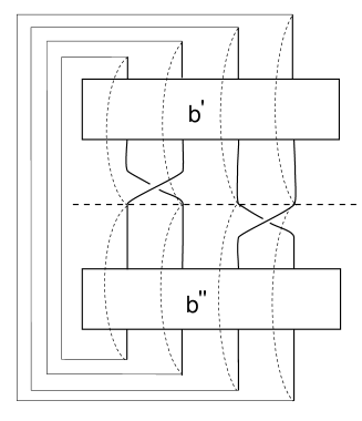
FIG. 10.: Construction of Brownian bridge for knots.

Returning the the group $B_{3}$, introduce normalized generators as follows

$$||\sigma_{j}^{\pm 1}||=(\det\sigma_{j}^{\pm 1})^{-1}\sigma_{j}^{\pm 1}.$$

To neglect the insignificant commutative factor dealing with norm of matrices $\sigma_{1}$ and $\sigma_{2}$. Now we can rewrite the power of Alexander invariant (Eq.(III.14)) in the form

$$\eta=\left[\#(+)-\#(-)\right]+\overline{\eta}$$ (III.28)

where $\#(+)$ and $\#(-)$ are numbers of generators $\sigma_{{\alpha}_{j}}$ or $\sigma_{{\alpha}_{j}}^{-1}$ in a given braid and $\overline{\eta}$ is the power of the normalized matrix product $\prod^{N}_{j=1}||\sigma_{{\alpha}_{j}}||$. The condition of Brownian bridge implies $\eta=0$ (i.e. $\#(+)-\#(-)=0$ and $\overline{\eta}=0$).

Write

$$||\sigma_{1}||=T(t);\qquad||\sigma_{2}||=T^{-1}(t)S(t)T^{-1}(t)$$ (III.29)

where $T(t)$ and $S(t)$ are the generators of the “$t$-deformed” group $PSL_{t}(2,\rm{\sf ZZ\hskip 1.70717pt})$

$$\begin{array}[]{ccc}\displaystyle T(t)&=&\left(\begin{array}[]{cc}(-t)^{1/2}&0\\ 0&(-t)^{-1/2}\end{array}\right)\left(\begin{array}[]{cc}1&(-t)^{-1}\\ 0&1\end{array}\right);\vskip 6.0pt plus 2.0pt minus 2.0pt\\ \displaystyle S(t)&=&\left(\begin{array}[]{cc}(-t)^{-1/2}&0\\ 0&(-t)^{1/2}\end{array}\right)\left(\begin{array}[]{rc}0&1\\ -1&0\end{array}\right)\end{array}$$ (III.30)

The group $PSL_{t}(2,\rm{\sf ZZ\hskip 1.70717pt})$ preserves the relations of the group $PSL(2,\rm{\sf ZZ\hskip 1.70717pt})$ unchanged, i.e., $(T(t)S(t))^{3}=S^{4}(t)=T(t)S^{2}(t)T^{-1}(t)S^{-2}(t)=1$ (compare to Eq.(III.19)). Hence, if we construct the graph $C(\Gamma_{t})$ for the group $PSL_{t}(2,\rm{\sf ZZ\hskip 1.70717pt})$ connecting the neighboring images of an arbitrary element from the fundamental domain, we ultimately come to the conclusion that the graphs $C(\Gamma_{t})$ and $C(\Gamma)$ (fig.9) are topologically equivalent. This is the direct consequence of the fact that group $B_{3}$ is the central extension of $PSL(2,\rm{\sf ZZ\hskip 1.70717pt})$. It should be emphasized that the metric properties of the graphs $C(\Gamma_{t})$ and $C(\Gamma)$ differ because of different embeddings of groups $PSL_{t}(2,\rm{\sf ZZ\hskip 1.70717pt})$ and $PSL(2,\rm{\sf ZZ\hskip 1.70717pt})$ into the complex plane.

Thus, the matrix product $\prod^{N}_{j=1}||\sigma_{{\alpha}_{j}}||$ for the uniform distribution of braid generators is in one-to-one correspondence with the $N$-step random walk along the graph $C(\Gamma)$. Its power coincides with the respective geodesics length along the backbone graph $C(\gamma)$. Thus we conclude that limit distribution of random walks on the group $B_{3}$ in terms of normalized generators (III.29) is given by Eq.(III.25) where $k$ should be regarded as the power of the product $\prod^{N}_{\alpha=1}||\sigma_{{\alpha}_{j}}||$. Hence we come to the following statement.

Take a set of knots obtained by closure of $B_{3}$-braids of length $N$ with the uniform distribution over the generators. The conditional probability distribution $U(\overline{\eta},m|N)$ for the normalized complexity $\overline{\eta}$ of Alexander polynomial invariant (see (III.28)) has the Gaussian behavior and is given by Eq.(III.26) where $k=\overline{\eta}$.

B Random walks on locally free groups

We aim at getting the asymptotic of conditional limit distributions of BB on the braid group $B_{n}$. For the case $n>3$ it presents a problem which is unsolved yet. However we can estimate limit probability distributions of BB on $B_{n}$ considering the limit distributions of random walks on the so-called “local groups” ([48, 44, 52, 53, 54]).

The group ${\cal LF}_{n+1}(d)$ we call the locally free if the generators, $\{f_{1},\ldots,f_{n}\}$ obey the following commutation relations:

(a) Each pair $(f_{j},f_{k})$ generates the free subgroup of the group ${\cal F}_{n}$ if $|j-k|<d$;

(b) $f_{j}f_{k}=f_{k}f_{j}$ for $|j-k|\geq d$.

(Below we restrict ourselves to the case $d=2$ where ${\cal LF}_{n+1}(2)\equiv{\cal LF}_{n+1}$).

The limit probability distribution for the $N$-step random walk ($N\gg 1$) on the group ${\cal F}_{n+1}$ to have the minimal irreducible length $\mu$ is

$$\begin{array}[]{ll}\displaystyle{\cal P}(\mu,N)\simeq\frac{\rm const}{N^{3/2}}e^{-N/6}\,\mu\sinh\mu\exp\left(-\frac{3\mu^{2}}{2N}\right)&(n=3)\vskip 6.0pt plus 2.0pt minus 2.0pt\\ \displaystyle{\cal P}(\mu,N)\simeq\frac{1}{2\sqrt{14\pi N}}\exp\left\{-\frac{8}{7N}\left(\mu-\frac{3}{4}N\right)^{2}\right\}&(n\gg 1)\end{array}$$ (III.31)

We propose two independent approaches valid in two different cases: (1) for $n=3$ and (2) for $n\gg 1$.

(1) The following geometrical image seems useful. Establish the one-to-one correspondence between the random walk in some $n$-dimensional Hilbert space ${\cal LH}^{n}(x_{1},\ldots,x_{n})$ and the random walk on the group ${\cal LF}_{n+1}$, written in terms of generators $\{f_{1},\ldots,f_{n}^{-1}\}$. To be more specific, suppose that when a generator, say, $f_{j}$, (or $f_{j}^{-1}$) is added to the given word in ${\cal LF}_{n}$, the walker makes one unit step towards (backwards for $f_{j}^{-1}$) the axis $[0,x_{j}[$ in the space ${\cal LH}^{n}(x_{1},\ldots,x_{n})$.

Now the relations (a)-(b) of the definition of the locally free group could be reformulated in terms of metric properties of the space ${\cal LH}^{n}$. Actually, the relation (b) indicates that successive steps along the axes $[0,x_{j}[$ and $[0,x_{k}[$ $(|j-k|\geq 2)$ commute, hence the section $(x_{j},x_{k})$ of the space ${\cal LH}^{n}$ is flat and has the Euclidean metric $dx_{j}^{2}+dx_{k}^{2}$. Situation with the random trajectories in the sections $(x_{j},x_{j\pm 1})$ of the Hilbert space ${\cal LH}^{n}$ appears to be completely different. Here the steps of the walk obey the free group relations (a) and the walk itself is mapped to the walk on the Cayley tree. It is well known that Cayley tree can be uniformly embedded (without gaps and selfintersections) into the 3-pseudosphere which gives the representation of the non-Euclidean plane with the constant negative curvature. Thus, sections $(x_{j},x_{j+1})$ have the metric of Lobachevskii plane which can be written in the form $\frac{1}{x_{j}^{2}}(dx_{j}^{2}+dx_{j+1}^{2})$.

For the group ${\cal LF}_{4}$ these arguments result in the following metric of appropriate space ${\cal LH}^{(3)}$

$$ds^{2}=\frac{dx_{1}^{2}+dx_{2}^{2}+dx_{3}^{2}}{x_{2}^{2}}$$ (III.32)

Actually, the space section $(x_{1},x_{3})$ is flat whereas the space sections $(x_{1},x_{2})$ and $(x_{2},x_{3})$ have Lobachevskii plane metric. The noneuclidean (hyperbolic) distance between two points $M^{\prime}$ and $M^{\prime\prime}$ in the space ${\cal H}^{3}$ is defined as follows

$$\cosh\mu(M^{\prime}M^{\prime\prime})=1+\frac{1}{x_{2}(M^{\prime})x_{2}(M^{\prime\prime})}\sum_{i=1}^{3}\left(x_{i}(M^{\prime})-x_{i}(M^{\prime\prime})\right)^{2}$$ (III.33)

where $\{x_{1},x_{2},x_{3}\}$ are the euclidean coordinates in the 3D-halfspace $x_{2}>0$ and $\mu$ is regarded as geodesics on a 4-pseudosphere (Lobachevskii space).

Some well known results concerning the limit behavior of random walks in spaces of constant negative curvature are reviewed in the next Section where solutions of the diffusion equations in the Lobachevskii plane and space are given by Eq.(III.58) and Eq.(III.60) correspondingly. Thus we can conclude that the distribution function for random walk in Lobachevskii space ${\cal P}_{s}(\mu,N)$ defined by Eqs.(III.60)-(III.63) gives also the probability for the $N$-letter random word (written in terms of uniformly distributed generators on ${\cal F}_{4}$) to have the primitive word of length $\mu$ (see Eq.(III.31)).

(2) For the group ${\cal LF}_{n+1}$ ($n\gg 1)$ we extract the limit behavior of the distribution function evaluating the probabilities to increase and to decrease the length of the primitive word if we randomly add one extra letter to the given word. We follow below the line proposed by J. Desbois [52, 54]

Let us point out the main steps of our computations:

• We generate randomly (with uniform probability distribution) the words of lengths $N\in[1000;20000]$, while the number of generators, $n$, varies in the interval $[3;200]$. The number of randomly generated words is of order of 1000.

• We reduce the given word till the minimal irreducible (primitive) word. This can be done by using the braid (or locally free) group relations. The numerical procedure is as follows. First, we try to push each braid generator in the word as far as possible to the left. Some reductions can occur after that. Then, we play the same game but in the opposite direction, pushing each braid generator to the right performing possible reductions of the word, then—to the left again and so on… If no reductions occur during two consecutive steps, we stop the process.

We compute the following quantities for braid and locally free groups:

The mean length of the shortest (primitive) word $\left<\mu\right>$

$$\left<\mu\right>=\frac{\sum\limits_{\mu=0}^{\infty}\mu Z(\mu,N)}{\sum\limits_{\mu=0}^{\infty}Z(\mu,N)}$$ (III.34)

and the variance $\mbox{Var}(\mu)$

$$\mbox{Var}(\mu)\equiv\bigl{<}\mu^{2}\bigr{>}-\bigl{<}\mu\bigr{>}^{2}=\frac{\sum\limits_{\mu=0}^{\infty}\mu^{2}Z(\mu,N)}{\sum\limits_{\mu=0}^{\infty}Z(\mu,N)}-\bigl{<}\mu\bigr{>}^{2}$$ (III.35)

The results of numerical simulations for the word statistics on braid ($B_{n}$) and locally free (${\cal LF}_{n}(d)$) groups are presented in the Table 1.

Table 1.

Groups	$B_{n}$		${\cal LF}_{n}(2)$		${\cal LF}_{n}(3)$		${\cal LF}_{n}(4)$
	$\frac{\left<\mu\right>}{N}$	$\frac{\mbox{Var}(\mu)}{N}$	$\frac{\left<\mu\right>}{N}$	$\frac{\mbox{Var}(\mu)}{N}$	$\frac{\left<\mu\right>}{N}$	$\frac{\mbox{Var}(\mu)}{N}$	$\frac{\left<\mu\right>}{N}$	$\frac{\mbox{Var}(\mu)}{N}$
n=3	0.29	0.85	0.50	0.76	0.50	0.76	0.50	0.75
n=5	0.49	0.77	0.60	0.63	0.71	0.48	0.75	0.46
n=10	0.56	0.63	0.65	0.56	0.77	0.40	0.82	0.34
n=20	0.59	0.63	0.66	0.54	0.79	0.39	0.84	0.29
n=50	0.61	0.61	0.67	0.56	0.80	0.38	0.85	0.27
n=100	0.61	0.61	0.67	0.52	0.80	0.36	0.86	0.26
n=200	0.61	0.60	0.67	0.53	0.80	0.35	0.86	0.26

The maximal standard deviations in the Table 1 (and everywhere below) are:

$$\left\{\begin{array}[]{ll}\pm 0.01&\mbox{for the mean value $\left<\mu\right>/N$}\\ \pm 0.05&\mbox{for the variance $\mbox{Var}(\mu)/N$}\end{array}\right.$$

C Analytic Results for Random Walks on Locally Free Group

Let us estimate now the quantities $\left<\mu\right>/N$ and $\mbox{Var}(\mu)/N$ analytically. We present below two different approaches called ”dynamical” and ”statistical”. The ”dynamical” approach is based on simple estimation of the probability to reduce the primitive word by random adding one extra letter. The estimate obtained by this method is in very good agreement with corresponding numerical simulations. However the ”statistical” approach dealing with rigorous enumeration of all nonequivalent primitive words in the locally free group ${\cal LF}_{n}(d)$ leads to another answer. The rest of this section is devoted to the explanation of the abovementioned discrepancy.

Dynamical Consideration. Under the conditions

$$\begin{array}[]{c}n\gg 1\\ N\gg n^{2}\end{array}$$ (III.36)

we can easily develop the dynamical arguments which are in rather good agreement with the results of numerical simulations presented above. The last inequality in (III.36) ensures the conditions, sufficient for finding the limit probability distribution of Markov chains on the groups of $n$ generators. Actually, the number of letters in the word, $N$ should be much larger that the number of all possible pairs in the set of $2n$ letters. Only in this case the corresponding Markov process has the reliable distribution function. The number of pairs is of order $4n^{2}$, so we arrived at the inequality stated in (III.36).

Take a randomly generated $N$–letter word $W$. This word is characterized by the length of the primitive word $W_{p}$ (recall that $W_{p}$ is the length of the word $W$ obtained after all possible contractions allowed by the structure of the group ${\cal LF}_{n}(d)$).

Let us compute the probability $\pi(d)$ of the fact that the primitive word $W_{p}$ will be shortened in one letter after adding of the letter $f_{i}$ ($i\in[1,n]$) to the word $W$ from the right-hand side. It is easy to understand that the primitive word $W_{p}$ can be reduced if:

• The last letter in the word $W_{p}$ is just $f_{i}^{-1}$. The probability of such event is $\frac{1}{2n}$;

• The letter before the last in the word $W_{p}$ is $f_{i}^{-1}$ and the last letter commutes with the letter $f_{i}$. The probability of such event is $\frac{1}{2n}\left(1-\frac{4d-2}{2n}\right)$;

• The third letter from the right end of the word $W_{p}$ is $f_{i}^{-1}$ and two last letters commute with the letter $f_{i}$. The probability of such event is $\frac{1}{2n}\left(1-\frac{4d-2}{2n}\right)^{2}$;

• … and so on.

Finally we arrive at the following expression for the probability $\pi(d)$:

$$\pi(d)=\frac{1}{2n}\sum_{l=0}^{\infty}\left(1-\frac{4d-2}{2n}\right)^{l}=\frac{1}{4d-2}$$ (III.37)

The procedure described above assumes that the letters remaining in the word $W_{p}$ are uniformly distributed—as in the initial (nonreduced word $W$). The absence of ”boundary effects” is ensured by the condition (III.36).

Once having the probability $\pi(d)$, we can write down the master equation for the probability $P(\mu,N)$ of the fact that in randomly generated $N$–letter word the primitive path has the length $\mu$

$$P(\mu,N+1)=(1-\pi(d))\,P(\mu-1,N)+\pi(d)\,P(\mu+1,N)\qquad(\mu\geq 2)$$ (III.38)

where the relation between $P(\mu,N)$ and the partition function $Z(\mu,N)$ introduced above is as follows

$$P(\mu,N)=\frac{Z(\mu,N)}{\sum\limits_{\mu=0}^{\infty}Z(\mu,N)}$$

The recursion relation (III.38) coincides with the equation describing the random walk on the halfline with the drift from the origin or, what is the same, with the equation describing the random walk on the simply Cayley tree with the coordinational number

$$z_{\rm eff}=\frac{1}{\pi(d)}=4d-2$$ (III.39)

Taking into account the last analogy we can complete the Eq.(III.38) by the boundary conditions

$$\begin{array}[]{l}P(\mu=1,N+1)=P(\mu=0,N)+\pi(d)\,P(\mu=2,N)\\ P(\mu=0,N+1)=\pi P(\mu=1,N)\\ P(\mu,N=0)=\delta_{\mu,0}\end{array}$$ (III.40)

It is noteworthy that these equations are written just for the Cayley tree with $z_{\rm eff}$ branches. The actual structure of the graph corresponding to the group ${\cal LF}_{n}(d)$ is much more complex, thus Eqs.(III.40) should be regarded as an aproximation. However the exact form of boundary conditions does not influence the asymptotic solution of Eq.(III.38) in vicinity of the maximum of the distribution function:

$$P(\mu,N)\simeq\frac{1}{2\sqrt{2\pi(z_{\rm eff}-1)N}}\exp\left\{-\frac{z_{\rm eff}^{2}}{8(z_{\rm eff}-1)N}\left(\mu-\frac{z_{\rm eff}-2}{z_{\rm eff}}N\right)^{2}\right\}$$ (III.41)

Thus, we find

$$\begin{array}[]{l}\displaystyle\frac{\left<\mu(d)\right>}{N}\simeq\frac{z_{\rm eff}-2}{z_{\rm eff}}=\frac{2d-2}{2d-1}\vskip 6.0pt plus 2.0pt minus 2.0pt\\ \displaystyle\frac{\mbox{Var}(\mu,d)}{N}\simeq\frac{4(z_{\rm eff}-1)}{z_{\rm eff}^{2}}=\frac{4d-3}{(2d-1)^{2}}\end{array}$$ (III.42)

Substituting in Eq.(III.42) $d=2,3,4$ we get the following numerical values:

$$\begin{array}[]{ll}\displaystyle\frac{\left<\mu(d)\right>}{N}=\frac{2}{3};\quad\displaystyle\frac{\mbox{Var}(\mu,d)}{N}=\frac{5}{9}&\quad\mbox{for $d=2$}\vskip 6.0pt plus 2.0pt minus 2.0pt\\ \displaystyle\frac{\left<\mu(d)\right>}{N}=\frac{4}{5};\quad\displaystyle\frac{\mbox{Var}(\mu,d)}{N}=\frac{9}{25}&\quad\mbox{for $d=3$}\vskip 6.0pt plus 2.0pt minus 2.0pt\\ \displaystyle\frac{\left<\mu(d)\right>}{N}=\frac{6}{7};\quad\displaystyle\frac{\mbox{Var}(\mu,d)}{N}=\frac{13}{49}&\quad\mbox{for $d=4$}\end{array}$$

what is in the excellent agreement with the asymptotic values ($n\gg 1$) from the Table 1 for the same groups.

Another statistical problem appears when we are interested in the consideration of the target space of the group ${\cal LF}_{n+1}$, i.e. in the evaluation of the number of nonequivalent primitive words in the froup ${\cal LF}_{n+1}$ (see for details [53]).

Let $V_{n}(\mu)$ be the number of all nonequivalent primitive words of length $\mu$ on the group ${\cal LF}_{n+1}$. When $\mu\gg 1$, $V_{n}(\mu)$ has the following asymptotic:

$$V_{n}(\mu)=\mbox{const}\left[1+2\left(3-\frac{4\pi^{2}}{n^{2}}\right)\right]^{\mu};\qquad n\gg 1$$ (III.43)

To get Eq.(III.43) we write each primitive word $W_{p}$ of length $\mu$ in the group ${\cal LF}_{n+1}$ in the so-called normal order (all $f_{\alpha_{i}}$ are different) similar to so-called ”symbolic dynamics” used in consideration of chaotic systems

$$W_{p}=\left(f_{\alpha_{1}}\right)^{m_{1}}\left(f_{\alpha_{2}}\right)^{m_{2}}\ldots\left(f_{\alpha_{s}}\right)^{m_{s}}$$ (III.44)

where $\displaystyle\sum_{i=1}^{s}|m_{i}|=\mu\;(m_{i}\neq 0\;\forall\;i;\;1\leq s\leq\mu$) and sequence of generators $f_{\alpha_{i}}$ in Eq.(III.44) for all $f_{{\alpha}_{i}}$ satisfies the following local rules:

• If $f_{\alpha_{i}}=f_{1}$, then $f_{\alpha_{i+1}}\in\left\{f_{2},f_{3},\ldots f_{n-1}\right\}$;

• If $f_{\alpha_{i}}=f_{k}$ ($1<k\leq n-1$), then $f_{\alpha_{i+1}}\in\left\{f_{k-1},f_{k+1},\ldots f_{n-1}\right\}$;

• If $f_{\alpha_{i}}=f_{n}$, then $f_{\alpha_{i+1}}=f_{n-1}$.

These local rules prescribe the enumeration of all distinct primitive words. If the sequence of generators in the primitive word $W_{p}$ does not satisfy the rules (i)-(iii), we commute the generators in the word $W_{p}$ up the normal order is restored. Hence, the normal order representation provides us with the unique coding of all nonequivalent primitive words in the group ${\cal LF}_{n+1}$.

The calculation of the number of distinct primitive words, $V_{n}(\mu)$, of the given length $\mu$ is rather straightforward:

$$V_{n}(\mu)=\sum_{s=1}^{\mu}R(s)\mathop{{\sum}^{\prime}}_{\{m_{1},\ldots,m_{s}\}}\Delta\left[\sum_{i=1}^{s}|m_{i}|-\mu\right]$$ (III.45)

where $R(s)$ is the number of all distinct sequences of $s$ generators taken from the set $\{f_{1},\ldots,f_{n}\}$ and satisfying the local rules (i)-(iii) while the second sum gives the number of all possible representations of the primitive path of length $\mu$ for the fixed sequence of generators (“prime” means that the sum runs over all $m_{i}\neq 0$ for $1\leq i\leq s$; $\Delta$ is the Kronecker $\Delta$-function).

It should be mentioned that the local rules (i)-(iii) define the generalized Markov chain with the states given by the $n\times n$ coincidence matrix $\hat{T}_{n}$ where the rows and columns correspond to the generators $f_{1},\ldots,f_{n}$:

$$\hat{T}_{n}(d)={\begin{tabular}[]{|c||c|c|c|c|c|c|c|}\hline\cr\rule{0.0pt}{12.0pt}&$f_{1}$&$f_{2}$&$f_{3}$&$f_{4}$&$\ldots$&$f_{n-1}$&$f_{n}$\\ \hline\cr\rule{0.0pt}{2.0pt}&&&&&&&\\ \hline\cr\rule{0.0pt}{12.0pt} $f_{1}$&0&1&1&1&$\ldots$&1&1\\ \hline\cr\rule{0.0pt}{12.0pt} $f_{2}$&1&0&1&1&$\ldots$&1&1\\ \hline\cr\rule{0.0pt}{12.0pt} $f_{3}$&1&1&0&1&$\ldots$&1&1\\ \hline\cr\rule{0.0pt}{12.0pt} $f_{4}$&0&1&1&0&$\ldots$&1&1\\ \hline\cr$\vdots$&$\vdots$&$\vdots$&$\vdots$&$\vdots$&$\ddots$&$\vdots$&$\vdots$\\ \hline\cr\rule{0.0pt}{12.0pt} $f_{n-1}$&0&0&0&0&$\ldots$&0&1\\ \hline\cr\rule{0.0pt}{12.0pt} $f_{n}$&0&0&0&0&$\ldots$&1&0\\ \hline\cr\end{tabular}}$$ (III.46)

The number of all distinct normally ordered sequences of words of length $s$ with allowed commutation relations is given by the following partition function

$$R_{n}(s,d)={\bf v}_{\mbox{in}}\left[\hat{T}_{n}(d)\right]^{s}{\bf v}_{\mbox{out}}$$ (III.47)

where

$${\bf v}_{\mbox{in}}=(\;\overbrace{1\;1\;1\;\ldots\;1}^{n}\;)\qquad\mbox{and}\qquad{\bf v}_{\mbox{out}}=\left.\left({\begin{array}[]{c}1\\ 1\\ 1\\ \vdots\\ 1\end{array}}\right)\right\}n$$ (III.48)

Supposing that the main contribution in Eq.(III.45) results from $s\gg 1$ we take for $R_{n}(s)$ the following asymptotic expression

$$R_{n}(s)\Big{|}_{s\gg 1}=\left(\lambda_{n}^{max}\right)^{s};\qquad\lambda_{n}^{max}=3-\frac{4\pi^{2}}{n^{2}}+O\left(\frac{1}{n^{3}}\right)$$ (III.49)

where $\lambda_{n}^{max}$ is the highest eigenvalue of the matrix $\hat{T}_{n}$ ($n\gg 1$).

The remaining sum in Eq.(III.45) is independent of $R(s)$, so its calculation is trivial:

$$\mathop{{\sum}^{\prime}}_{\{m_{1},\ldots,m_{s}\}}\Delta\left[\sum_{i=1}^{s}|m_{i}|-\mu\right]=2^{s}\frac{(\mu-1)!}{(s-1)!(\mu-s)!}$$ (III.50)

Collecting all terms in Eq.(III.45) and evaluating the sum over $s$ we arrive at Eq.(III.43). The value $V_{n}(\mu,d)$ is growing exponentially fast with $\mu$ and the ”speed” of this grows is clearly represented by the fraction

$$z_{\rm eff}-1=\frac{V_{n}(\mu+1)}{V_{n}(\mu)}\bigg{|}_{\mu\gg 1}\simeq 7-\frac{8\pi^{2}}{n^{2}}$$ (III.51)

where $z_{\rm eff}$ is the coordinational number of effective tree associated with the locally free group.

Thus, the random walk on the group ${\cal LF}_{n+1}$ can be viewed as follows. Take the free group $\Gamma_{n}$ with generators $\{\tilde{f}_{1},\ldots,\tilde{f}_{n}\}$ where all $\tilde{f}_{i}$ ($1\leq i\leq n$) do not commute. The group $\Gamma_{n}$ has a structure of $2n$-branching Cayley tree, $C(\Gamma_{n}),$ where the number of distinct words of length $\mu$ is equal to $\tilde{V}_{n}(\mu)$,

$$\tilde{V}_{n}(\mu)=2n(2n-1)^{\mu-1}$$ (III.52)

The graph $C({\cal LF}_{n+1})$ corresponding to the group ${\cal LF}_{n+1}$ can be constructed from the graph $C(\Gamma_{n})$ in accordance with the following recursion procedure: (a) Take the root vertex of the graph $C(\Gamma_{n})$ and consider all vertices on the distance $\mu=2$. Identify those vertices which correspond to the equivalent words in group ${\cal LF}_{n+1}$; (b) Repeat this procedure taking all vertices at the distance $\mu=(1,2,\ldots)$ and “gluing” them at the distance $\mu+2$ according to the definition of the locally free group. By means of the described procedure we raise a graph which in average has $z_{\rm eff}-1$ distinct branches leading to the ”next coordinational sphere”. Thus this graph coincides (in average) with $z_{\rm eff}$-branching Cayley tree.

Although the local structure of the graph $C({\cal LF}_{n+1})$ is very complex, Eq.(III.51) enables us to find the asymptotic of the random walk on the graph $C({\cal LF}_{n+1})$. Once having $z_{\rm eff}$, we can write down the master equation for the probability ${\cal P}(\mu,N)$ to find the walker at the distance $\mu$ from the origin after $N$ random steps on the graph $C({\cal LF}_{n+1})$

$${\cal P}(\mu,N+1)=(1-\frac{1}{z_{\rm eff}})\,P(\mu-1,N)+\frac{1}{z_{\rm eff}}\,P(\mu+1,N)\qquad(\mu\geq 2)$$ (III.53)

The recursion relation (III.53) coincides with the equation describing the random walk on the half-line with the drift from the origin. Taking into account this analogy we can complete the Eq.(III.53) by the boundary conditions [52]. However the exact form of boundary conditions does not influence the asymptotic solution of Eq.(III.53) in vicinity of the maximum of the distribution function:

$${\cal P}(\mu,N)\simeq\frac{1}{2\sqrt{2\pi(z_{\rm eff}-1)N}}\exp\left\{-\frac{z_{\rm eff}^{2}}{8(z_{\rm eff}-1)N}\left(\mu-\frac{z_{\rm eff}-2}{z_{\rm eff}}N\right)^{2}\right\}$$

Thus we obtain the desired distribution function (Eq.(III.31)) for the primitive word length for the random walk on the group ${\cal LF}_{n+1}$.

The Eq.(III.31) gives the estimation from below for the limit distribution of the primitive words on the group $B_{n}$ for $n\gg 1$.

We find further investigation of the random walks on the groups ${\cal LF}_{n+1}(d)$ for different values of $d$ very perspective. It should give insight for consideration of random walk statistics on “partially commutative groups”. Moreover, the set of problems considered there has deep relation with the spectral theory of random matrices.

D Brownian bridges on Lobachevskii plane and products of non-commutative random matrices

The problem of word enumeration on locally non-commutative group has evident connection with the statistics of Markov chains on graphs having the Cayley tree–like structure and, hence, with random walk statistics on the surfaces of a constant negative curvature. (We stressed once that the Cayley tree–like graphs are isometrically embedded in the surfaces of a constant negative curvature).

Recall that the distribution function, $P({\bf r},t)$, for the free random walk in D-dimensional Euclidean space obeys the standard heat equation:

$$\frac{\partial}{\partial t}P({\bf r},t)={\cal D}\Delta P({\bf r},t)$$

with the diffusion coefficient ${\cal D}=\frac{1}{2D}$ and appropriate initial and normalization conditions

$$\begin{array}[]{c}\displaystyle P({\bf r},t=0)=\delta({\bf r})\vskip 6.0pt plus 2.0pt minus 2.0pt\\ \displaystyle\int P({\bf r},t)d{\bf r}=1\end{array}$$

Correspondingly, the diffusion equation for the scalar density $P({\bf q},t)$ of the free random walk on a Riemann manifold reads (see [62] for instance)

$$\frac{\partial}{\partial t}P({\bf q},t)={\cal D}\frac{1}{\sqrt{g}}\frac{\partial}{\partial q_{i}}\left(\sqrt{g}\left(g^{-1}\right)_{ik}\frac{\partial}{\partial q_{k}}\right)P({\bf q},t)$$ (III.54)

where

$$\begin{array}[]{c}\displaystyle P({\bf q},t=0)=\delta({\bf q})\vskip 6.0pt plus 2.0pt minus 2.0pt\\ \displaystyle\int\sqrt{g}P({\bf q},t)d{\bf q}=1\end{array}$$ (III.55)

and $g_{ik}$ is the metric tensor of the manifold; $g=\det g_{ik}$.

Eq.(III.54) has been subjected to thorough analysis for the manifolds of the constant negative curvature. Below we reproduce the corresponding solutions for the best known cases: for 2D– and 3D–Lobachevskii spaces (often referred to as 3– and 4–pseudospheres) labelling them by indices “$p\,$” and “$s\,$” for 2D– and 3D–cases correspondingly.

For the Lobachevskii plane one has

$$||g_{ik}||=\left|\left|\begin{array}[]{cc}1&0\vskip 6.0pt plus 2.0pt minus 2.0pt\\ 0&\sinh^{2}\mu\end{array}\right|\right|$$ (III.56)

where $\mu$ stands for the geodesics length on 3-pseudosphere. The corresponding diffusion equation now reads

$$\frac{\partial}{\partial t}P_{p}(\mu,\varphi,t)={\cal D}\left(\frac{\partial^{2}}{\partial\mu^{2}}+\coth\mu\frac{\partial}{\partial\mu}+\frac{1}{\sinh^{2}\mu}\frac{\partial^{2}}{\partial\varphi^{2}}\right)P_{p}(\mu,\varphi,t)$$ (III.57)

The solution of Eq.(III.57) is believed to have the following form

$$\begin{array}[]{lll}P_{p}(\mu,t)&=&\displaystyle\frac{e^{-\frac{t{\cal D}}{4}}}{4\pi\sqrt{2\pi(t{\cal D})^{3}}}\int_{\mu}^{\infty}\frac{\xi\exp\left(-\frac{\xi^{2}}{4t{\cal D}}\right)}{\sqrt{\cosh\xi-\cosh\mu}}d\xi\vskip 6.0pt plus 2.0pt minus 2.0pt\\ &\simeq&\displaystyle\frac{e^{-\frac{t{\cal D}}{4}}}{4\pi t{\cal D}}\left(\frac{\mu}{\sinh\mu}\right)^{1/2}\exp\left(-\frac{\mu^{2}}{4t{\cal D}}\right)\end{array}$$ (III.58)

For the Lobachevskii space the corresponding metric tensor is

$$||g_{ik}||=\left|\left|\begin{array}[]{ccc}1&0&0\vskip 6.0pt plus 2.0pt minus 2.0pt\\ 0&\sinh^{2}\mu&0\vskip 6.0pt plus 2.0pt minus 2.0pt\\ 0&0&\sinh^{2}\mu\sin^{2}\theta\end{array}\right|\right|$$ (III.59)

Substituting Eq.(III.54) for Eq.(III.59) we have

$$P_{s}(\mu,t)=\frac{e^{-t{\cal D}}}{8\pi\sqrt{\pi(t{\cal D})^{3}}}\frac{\mu}{\sinh\mu}\exp\left(-\frac{\mu^{2}}{4t{\cal D}}\right)$$ (III.60)

For the first time this spherically symmetric solution of the heat equation (Eq.(III.54)) in the Lobachevskii space was received in [63].

In our opinion one fact must be given our attention. The distribution functions $P_{\rm p}(\mu,t)$ and $P_{\rm s}(\mu,t)$ give the probabilities to find the random walk starting at the point $\mu=0$ after time $t$ in some specific point located at the distance $\mu$ in corresponding noneuclidean space. The probability to find the terminal point of a random walk after time $t$ somewhere at the distance $\mu$ is

$${\cal P}_{\rm p,s}(\mu,t)=P_{\rm p,s}(\mu,t){\cal N}_{\rm p,s}(\mu)$$ (III.61)

where

$${\cal N}_{\rm p}(\mu)=\sinh\mu$$ (III.62)

is the perimeter of circle of radius $\mu$ on the Lobachevskii plane and

$${\cal N}_{\rm s}(\mu)=\sinh^{2}\mu$$ (III.63)

is the area of sphere of radius $\mu$ in the Lobachevskii space.

The difference between $P_{\rm p,s}$ and ${\cal P}_{\rm p,s}$ is insignificant in euclidean geometry, whereas in the noneuclidean space it becomes dramatic because of the consequences of the behavior of Brownian bridges in spaces on constant negative curvature.

Using the definition of the Brownian bridge, let us calculate the probabilities to find the $N$-step random walk (starting at $\mu=0$) after first $t$ steps at the distance $\mu$ in the Lobachevskii plane (space) under the condition that it returns to the origin on the last step. These probabilities are ($N\to\infty$)

$$\begin{array}[]{l}\displaystyle{\cal P}_{\rm p}(\mu,t|0,N)=\frac{P_{\rm p}(\mu,t){\cal P}_{\rm p}(\mu,N-t)}{P_{\rm p}(0,t)}=\frac{N}{4\pi{\cal D}t(N-t)}\mu\exp\left\{-\frac{\mu^{2}}{4{\cal D}}\left(\frac{1}{t}+\frac{1}{N-t}\right)\right\}\vskip 6.0pt plus 2.0pt minus 2.0pt\\ \displaystyle{\cal P}_{\rm s}(\mu,t|0,N)=\frac{P_{\rm s}(\mu,t){\cal P}_{\rm s}(\mu,N-t)}{P_{\rm s}(0,t)}=\frac{N^{3/2}}{8\pi t^{3/2}(N-t)^{3/2}}\mu^{2}\exp\left\{-\frac{\mu^{2}}{4{\cal D}}\left(\frac{1}{t}+\frac{1}{N-t}\right)\right\}\end{array}$$ (III.64)

Hence we come to the standard Gaussian distribution function with zero mean.

Equations (III.64) describing the random walk on the Riemann surface of constant negative curvature have direct application to the conditional distributions of Lyapunov exponents for products of some non-commutative matrices. Let us consider the first of Eqs.(III.64). Changing the variables $\mu=\ln\frac{1+|z|}{1-|z|};\quad\varphi=\arg z$ where $z=x+iy;\,\bar{z}=x-iy$ we map the 3–pseudosphere $(\mu,\varphi)$ onto the unit disk $|z|<1$ known as the Poincare representation of the Lobachevskii plane. The corresponding conformal metric reads $dl^{2}=\frac{4\;dzd\bar{z}}{\left(1-|z|^{2}\right)^{2}}$. Using the conformal transform $\displaystyle z=\frac{1+iw}{1-iw}$ we recover the so-called Klein representation of Lobachevskii plane, where $dl^{2}=-\frac{4\;dwd\bar{w}}{\left(w-\bar{w}\right)^{2}}$ and the model is defined in Im$w>0$ ($w=u+iv;\,\bar{w}=u-iv$).

The following relations can be verified using conformal representations of the Lobachevskii plane metric (see, for instance, [17]). The fractional group of motions of Lobachevskii plane is isomorphic to:

(i) the group $SU(1,1)/\pm 1\equiv PSU(1,1)$ in the Poincare model; (ii) the group $SL(2,{\rm{\sf RI\hskip 5.97508pt}})/\pm 1\equiv PSL(2,\rm{\sf RI\hskip 5.97508pt})$ in the Klein model.

Moreover, it is known (see, for example, [34]) that the Lobachevskii plane $H$ can be identified with the group $SL(2,{\rm{\sf RI\hskip 5.97508pt}})/SO(2)$. This relation enables us to resolve (at least qualitatively) the following problem. Take the Brownian bridge on the group ${\cal H}=SL(2,{\rm{\sf RI\hskip 5.97508pt}})/SO(2)$, i.e. demand the products of $N$ independent random matrices $\widehat{\cal M}_{k}\in{\cal H}\;(0\leq k\leq N)$ to be identical to the unit matrix. Consider the limit distribution of the Lyapunov exponent, $\hat{\delta}$, for the first $m$ matrices in that products. To have a direct mapping of this problem on the random walk in the Lobachevskii plane, write the corresponding stochastic recursion equation for some vector $\displaystyle{\bf W}_{k}={u_{k}\choose v_{k}}$

$${\bf W}_{k+1}=\widehat{\cal M}_{k}{\bf W}_{k};\qquad{\bf W}_{0}={1\choose 1}$$ (III.65)

where ${\cal M}_{k}\in{\cal H}$ for all $k\in[1,N]$. The BB–condition means that

$${\bf W}_{N}={\bf W}_{1}\quad\mbox{for $N\gg 1$}$$ (III.66)

Let us consider the simplest case

$$\widehat{\cal M}_{k}=1+\widehat{M}_{k};\qquad\mbox{norm}[\widehat{M}_{k}]\ll 1$$ (III.67)

In this case the discrete dynamic equation (III.65) can be replaced by the differential one. Its stationary measure is determined by the corresponding Fokker-Plank equation (III.54). The Lyapunov exponent, $\hat{\delta}$ of product of random matrices $\widehat{\cal M}$ coincides with the length of geodesics in the Klein representation of the Lobachevskii plane. Hence, under the conditions (III.66), (III.67) we have for $\hat{\delta}$ the usual Gaussian distribution coinciding with the first of Eq.(III.64). Without the BB–condition (i.e. for “open walks”) we reproduce the standard Fürstenberg behavior [39].

Although this consideration seems rather crude (for details see Appendix A), it clearly shows the origin of the main result:

The “Brownian bridge” condition for random walks in space of constant negative curvature makes the space “effectively flat” turning the corresponding limit probability distribution for random walks to the ordinary central limit distribution.

The question whether this result is valid for the case of the random walk in noneuclidean spaces of non-constant negative curvature still remains.

Finally we would like to introduce some conjectures which naturally generalize our consideration.

The complexity $\eta$ of any known algebraic invariants (Alexander, Jones, HOMFLY) for the knot represented by the $B_{n}$-braid of length $N$ with the uniform distribution over generators has the following limit behavior:

$$P(\eta,N)\sim\frac{{\rm const}}{N^{3/2}}\eta\exp\left(-\alpha(n)N+\beta(n)\eta-\frac{\eta^{2}}{\delta(n)N}\right)$$ (III.68)

where $\alpha(n),\;\beta(n),\;\delta(n)$ are numerical constants depending on $n$ only.

The knot complexity $\eta$ in ensemble of Brownian bridges from the group $B_{n}$ shown in fig.10 has Gaussian distribution, where

$$\left<\overline{\eta}\right>=0;\qquad\left<\overline{\eta}^{2}\right>=\frac{1}{2}\delta(n)N$$ (III.69)

These conjectures are to be proven yet. The main idea is to employ the relation between the knot complexity $\eta$, the length of the shortest noncontractible word and the length of geodesics on some hyperbolic manifold.

IV Conformal methods in statistics of random walks with topological constraints

The last few years have been marked by considerable progress in understanding the relationship between Chern-Simons topological field theory, construction of algebraic knot and link invariants and conformal field theory (see, for review, [64]).

Although the general concepts have been well elaborated in the field-theoretic context, their application in the related areas of mathematics and physics, such as, for instance, probability theory and statistical physics of chain-like objects is highly limited.

The present Section is mainly concerned with the conformal methods in statistical analysis which allow us to correlate problems discussed in Chapters 1 and 2 and the limit distributions of random walks on multiconnected Riemann surfaces. To be more specific, we show on the level of differential equations how simple geometrical methods can be applied to construction of non-commutative topological invariants. The latter might serve as nonabelian generalizations of the Gauss linking numbers for the random walks on multi-punctured Riemann surfaces. We also study the connection between the topological properties of random walks on the double punctured plane and behavior of four-point correlation functions in the conformal theory with central charge $c=-2$. The developed approach is applied to the investigation of statistics of 2D–random walks with multiple topological constraints. For instance, the methods presented here allow us to extract nontrivial critical exponents for the contractible (i.e., unentangled) random walks in the regular lattices of obstacles. Some of our findings support conjectures of Sections 2 and 3 and have direct application in statistics of strongly entangled polymer chains (see Section 5).

A Construction of nonabelian connections for $\Gamma_{2}$ and $PSL(2,\rm{\sf ZZ\hskip 1.70717pt})$ from conformal methods

We analyze the random walk of length $L$ with the effective elementary step $a$ ($a\equiv 1$) on the complex plane $z=x+iy$ with two points removed. Suppose the coordinates of these points being $M_{1}$ ($z_{1}=(0,0)$) and $M_{2}$ ($z_{2}=(c,0)$) ($c\equiv 1$). Such choice does not indicate the loss of generality because by means of simultaneous rescaling of the effective step, $a$, of the random walk and of the distance, $c$, between the removed points we can always obtain of any arbitrary values of $a$ and $c$.

Consider the closed paths on $z$ and attribute the generators $g_{1},\,g_{2}$ of some group $G$ to the turns around the points $M_{1}$ and $M_{2}$ if we move along the path in the clockwise direction (we apply $g_{1}^{-1},\,g_{2}^{-1}$ for counter-clockwise move)—see fig.11.

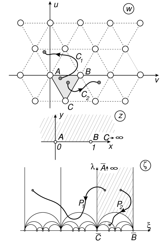
FIG. 11.: (a)—the double punctured complex plane $z$ with two basis loops $C_{1}$ and $C_{2}$ enclosing points $M_{1}$ and $M_{2}$; (b)—the universal covering $\zeta$ with fundamental domain corresponding to free group $\Gamma_{2}$. The contours $P_{1}$ and $P_{2}$ are the images of the loops $C_{1}$ and $C_{2}$.

The question is: what is the probability $P(\mu,L)$ for the random walk of length $L$ on the plane $z$ to form a closed loop with the shortest noncontractible word written in terms of generators $\{g_{1},g_{2},g_{1}^{-1},g_{2}^{-1}\}$ to have the length $\mu$ (see also Chapter 2).

Let the distribution function $P(\mu,L)$ be formally written as a path integral with a Wiener measure

$$\begin{array}[]{ll}\displaystyle P(\mu,L)=\frac{1}{\cal Z}\int\ldots\int{\cal D}\{z\}&\displaystyle\exp\left\{-\frac{1}{a^{2}}\int_{0}^{L}\left(\frac{dz(s)}{ds}\right)^{2}ds\right\}\vskip 6.0pt plus 2.0pt minus 2.0pt\\ &\times\delta\left[W\{g_{1},g_{2},g_{1}^{-1},g_{2}^{-1}|z\}-\mu\right]\end{array}$$ (IV.1)

where ${\cal Z}=\int P(\mu,L)d\mu$ and $W\{\ldots|z\}$ is the length of the shortest word on $G$ as a functional of the path on the complex plane.

Conformal methods enable us construct the connection and the topological invariant $W$ for the given group as well as to rewrite Eq.(IV.1) in a closed analytic form which is solvable at least in the limit $L\to\infty$.

Let $\zeta(z)$ be the conformal mapping of the double punctured plane $z=x+iy$ on the universal covering $\zeta=\xi+i\lambda$. The Riemann surface $\zeta$ is constructed in the following way. Make three cuts on the complex plane $z$ between the points $M_{1}$ and $M_{2}$, between $M_{2}$ and $(\infty)$ and between $(\infty)$ and $M_{1}$ along the line Im$z=0$. These cuts separate the upper (Im$z>0$) and lower (Im$z<0$) half-planes of $z$. Now perform the conformal transform of the half-plane Im$z>0$ to the fundamental domain of the group $G\{g_{1},g_{2}\}$—the curvilinear triangle lying in the half-plane Im$\zeta>0$ of the plane $\zeta$. Each fundamental domain represents the Riemann sheet corresponding to the fibre bundle above $z$. The whole covering space $\zeta$ is the unification of all such Riemann sheets.

The coordinates of initial and final points of any trajectory on universal covering $\zeta$ determine ([66]): (a) The coordinates of corresponding points on $z;$ (b) The homotopy class of any path on $z$. In particular, the contours on $\zeta$ are closed if and only if $W\{g_{1},g_{2}|z\}\equiv 1$, i.e. they belong to the trivial homotopy class.

Coordinates of ends of the trajectory on universal covering $\zeta$ can be used as the topological invariant for the path on double punctured plane $z$ with respect to the action of the group $G$.

Thus, we characterize the topological invariant, Inv$(C)$, of some closed directed path $C$ starting and ending in an arbitrary point $z_{0}\neq\{z_{1},z_{2},\infty\}$ on the plane $z$ by the coordinates of the initial, $\zeta_{\rm in}(z_{0})$, and final, $\zeta_{\rm fin}(z_{0})$, points of the corresponding contour $P$ in the covering space $\zeta$. The contour $P$ connects the images of the point $z_{0}$ on the different Riemann sheets. Write Inv${}_{(z)}(C)$ as a full derivative along the contour $C$:

$$\mbox{Inv}_{(z)}(C)\stackrel{{\scriptstyle def}}{{=}}\zeta_{\rm in}-\zeta_{\rm fin}=\oint_{C}{{d\zeta(z)}\over{dz}}dz$$ (IV.2)

The physical interpretation of the derivative $\displaystyle\frac{d\zeta(z)}{dz}$ is very straightforward. Actually, the invariant, Inv$(C)$, can be associated with the flux through the contour $C$ on the plane $(x,y)$:

$$\mbox{Inv}(C)\equiv\mbox{Inv}_{(x,y)}(C)=\oint_{C}\nabla\zeta(x,y){\bf n}d{\bf r}=\oint_{C}\nu\times\nabla\zeta(x,y){\bf v}(s)ds$$ (IV.3)

where: ${\bf n}$ is the unit vector normal to the curve $C$, $d{\bf r}={\bf e}_{x}dx+{\bf e}_{y}dy$ on the plane $(x,y)$; $\displaystyle{\bf v}(s)=\frac{d{\bf r}}{ds}$ denotes the ”velocity” along the trajectory; and $ds$ stands for the differential path length. Simple transformations used in Eq.(IV.3) are: (a) ${\bf n}d{\bf r}={\bf e}_{x}dy-{\bf e}_{y}dx=d{\bf r}\times\nu$; (b) $\nabla\zeta(x,y)(d{\bf r}\times{\bf\nu})=({\bf\nu}\times\nabla\zeta(x,y))d{\bf r}$, where ${\bf\nu}=(0,0,1)$ is the unit vector normal to the plane $(x,y)$.

The vector product

$${\bf A}(x,y)={\bf\nu}\times\nabla\zeta(x,y)$$ (IV.4)

can be considered a non-abelian generalization of the vector potential of a solenoidal ”magnetic field” normal to the plane $(x,y)$ and crossing it in the points $(x_{1},y_{1})$ and $(x_{2},y_{2})$. Thus, ${\bf A}$ defines the flat connection of the double punctured plane $z$ with respect to the action of the group $G$.

It is easy to show how the basic formulae (IV.2) and (IV.3) transform in case of commutative group $G_{\rm comm}\{g_{1},g_{2}\}$ which distinguishes only the classes of homology of the contour $C$ with respect to the removed points on the plane. The corresponding conformal transform is performed by the function $\zeta(z)=\ln(z-z_{1})+\ln(z-z_{2})$. This immediately gives the abelian connection and the Gauss linking number as a topological invariant:

$$\begin{array}[]{c}\displaystyle{\bf A}({\bf r})={\bf\nu}\times\sum_{j=\{1,2\}}\frac{{\bf r}-{\bf r}_{j}}{|{\bf r}-{\bf r}_{j}|^{2}};\vskip 6.0pt plus 2.0pt minus 2.0pt\\ \displaystyle\mbox{Inv}(C)=\oint_{C}A({\bf r})d{\bf r}=\sum_{j=\{1,2\}}\oint_{C}\frac{(y-y_{j})dx-(x-x_{j})dy}{(x-x_{j})^{2}+(y-y_{j})^{2}}=2\pi(n_{1}+n_{2})\end{array}$$

where $n_{1}$ and $n_{2}$ are the winding numbers of the path $C$ around the points $M_{1}$ and $M_{2}$ of the plane $(x,y)$.

Substituting Eq.(IV.1) written in the Euclidean coordinates $(x,y)$ for Eq.(IV.3) and using the Fourier transform for the $\delta$-function, we can rewrite equation (IV.1) as follows

$$P(\mu,L)=\frac{1}{2\pi}\int_{-\infty}^{\infty}e^{-iq\mu}P(q,L)dq$$ (IV.5)

where

$$P(q,L)=\frac{1}{\cal Z}\int\ldots\int{\cal D}\{{\bf r}\}\exp\left\{-\frac{1}{a^{2}}\int\limits_{0}^{L}\left(\left(\frac{d{\bf r}(s)}{ds}\right)^{2}-iq{\bf A}({\bf r})\frac{d{\bf r}(s)}{ds}\right)ds\right\}$$ (IV.6)

The function $P(q,L)$ coincides with the Green function $P({\bf r}_{0},{\bf r}={\bf r}_{0},q,L)$ of the non-stationary Schrödinger-like equation for the free particle motion in a ”magnetic field” with the vector potential (IV.4):

$$\frac{\partial}{\partial L}P({\bf r}_{0},{\bf r},q,L)-\left(\frac{1}{2a}{\bf\nabla}-iq{\bf A}({\bf r})\right)^{2}P({\bf r}_{0},{\bf r},q,L)=\delta(L)\delta({\bf r}-{\bf r}_{0})$$ (IV.7)

where $q$ plays a role of a ”charge” and the magnetic field is considered transversal, i.e. $\mbox{rot}{\bf A}({\bf r})=0$.

Describe now the constructive way of getting the desired conformal transform. The single-valued inverse function $z(\zeta)\equiv\zeta^{-1}(z)$ is defined in the fundamental domain of $\zeta$—the triangle $ABC$. The multivalued function $\phi(\zeta)$ is determined as follows:

– The function $\phi(\zeta)$ coincides with $z(\zeta)$ in the basic fundamental domain;

– In all other domains of the covering space $\zeta$ the function $\phi(\zeta)$ is analytically continued through the boundaries of these domains by means of fractional transformations consistent with the action of the group $G$.

Consider two basic contours $P_{1}$ and $P_{2}$ on $\zeta$ being the conformal images of the contours $C_{1}$ and $C_{2}$ (fig.11b). The function $\phi(z)$ ($z\neq\{z_{1},z_{2},\infty\}$) obeys the following transformations:

$$\phi\left[z\stackrel{{\scriptstyle C_{1}}}{{\rightarrow}}z\right]\rightarrow\tilde{\phi}_{1}(z)={{a_{1}\phi(z)+b_{1}}\over{c_{1}\phi(z)+d_{1}}};\;\phi\left[z\stackrel{{\scriptstyle C_{2}}}{{\rightarrow}}z\right]\rightarrow\tilde{\phi}_{2}(z)={{a_{2}\phi(z)+b_{2}}\over{c_{2}\phi(z)+d_{2}}}$$ (IV.8)

where

$$\left(\begin{array}[]{cc}a_{1}&b_{1}\\ c_{1}&d_{1}\end{array}\right)=g_{1};\qquad\left(\begin{array}[]{cc}a_{2}&b_{2}\\ c_{2}&d_{2}\end{array}\right)=g_{2}$$ (IV.9)

are the matrices of basic substitutions of the group $G\{g_{1},g_{2}\}$.

We assume $\zeta(z)$ to be a ratio of two fundamental solutions, $u_{1}(z)$, and, $u_{2}(z)$, of some second order differential equation with peculiar points $\{z_{1}=(0,0),z_{2}=(0,1),z_{3}=(\infty)\}$. As it follows from the analytic theory of differential equations [68], the solutions $u_{1}(z)$ and $u_{2}(z)$ undergo the linear transformations when the variable $z$ moves along the contours $C_{1}$ and $C_{2}$:

$$C_{1}:\,\left(\begin{array}[]{c}\tilde{u}_{1}(z)\\ \tilde{u}_{2}(z)\end{array}\right)=g_{1}\left(\begin{array}[]{c}u_{1}(z)\\ u_{2}(z)\end{array}\right);\quad C_{2}:\,\left(\begin{array}[]{c}\tilde{u}_{1}(z)\\ \tilde{u}_{2}(z)\end{array}\right)=g_{2}\left(\begin{array}[]{c}u_{1}(z)\\ u_{2}(z)\end{array}\right)$$ (IV.10)

The problem of restoring the form of differential equation knowing the monodromy matrices $g_{1}$ and $g_{2}$ of the group $G$ known as Riemann-Hilbert problem has an old history [68]. In our particular case we restrict ourselves with the well investigated groups $\Gamma_{2}$ (the free group) and $PSL(2,\rm{\sf ZZ\hskip 1.70717pt})$ (the modular group). (III.16). Thus, we have the following second-order differential equations:

$$z(z-1){{d^{2}}\over{dz^{2}}}u^{(f)}(z)+(2z-1){{d}\over{dz}}u^{(f)}(z)+{1\over 4}u^{(f)}(z)=0$$ (IV.11)

for the free group and

$$z(z-1){{d^{2}}\over{dz^{2}}}u^{(m)}(z)+\left({5\over 3}z-1\right){{d}\over{dz}}u^{(m)}(z)+{1\over{12}}u^{(m)}(z)=0$$ (IV.12)

for the modular group.

The function which performs the conformal mapping of the upper half-plane Im$z>0$ on the fundamental domain (the curvilinear triangle $ABC$) of the universal covering $\zeta$ now reads

$$\zeta(z)=\frac{u_{1}^{\rm(f,m)}(z)}{u_{2}^{(f,m)}(z)}$$ (IV.13)

where $u_{1,2}^{(f,m)}(z)$ and $u_{1,2}^{(f,m)}(z)$ are the basic solutions of (IV.11) and (IV.12) for $\Gamma_{2}$ and $PSL(2,\rm{\sf ZZ\hskip 1.70717pt})$ respectively.

As an example we give an explicit form of the complex potential $A(z)$ for the free group $\Gamma_{2}$. Substituting Eq.(IV.2) for Eq.(IV.13), we get

$$A(z)=\frac{d\zeta(z)}{dz}=\frac{1}{2(z-1)}\left(\frac{F_{1}(z)F_{4}(z)}{F_{2}^{2}(z)}-\frac{F_{3}(z)}{F_{2}(z)}\right)$$ (IV.14)

where

$$\begin{array}[]{rl}\displaystyle F_{1}(z)=\int\limits_{1}^{1/\sqrt{z}}\frac{d\kappa}{\sqrt{(1-\kappa^{2})(1-z\kappa^{2})}};&\displaystyle F_{2}(z)=\int\limits_{0}^{1}\frac{d\kappa}{\sqrt{(1-\kappa^{2})(1-z\kappa^{2})}}\vskip 6.0pt plus 2.0pt minus 2.0pt\\ \displaystyle F_{3}(z)=\int\limits_{1}^{1/\sqrt{z}}\sqrt{\frac{1-\kappa^{2}}{1-z\kappa^{2}}}d\kappa;&\displaystyle F_{4}(z)=\int\limits_{0}^{1}\sqrt{\frac{1-\kappa^{2}}{1-z\kappa^{2}}}d\kappa\end{array}$$

The asymptotic of (IV.14) is as follows

$$\frac{d\zeta(z)}{dz}\sim\left\{\begin{array}[]{cl}\displaystyle\frac{1}{z}&\qquad z\to 0\vskip 6.0pt plus 2.0pt minus 2.0pt\\ \displaystyle\frac{1}{z-1}&\qquad z\to 1\end{array}\right.$$

(compare to the abelian case).

B Random walk on double punctured plane and conformal field theory

The geometrical construction described in the previous section is evidently related to the conformal field theory. In the most direct way this relation could be understood as follows. The ordinary differential equations Eq.(IV.11) and Eq.(IV.12) can be associated with equations on the four-point correlation function of some (still not defined) conformal field theory. The question remains whether it is always possible to adjust the central charge $c$ of the corresponding Virosoro algebra and the conformal dimension $\Delta$ of the critical theory to the coefficients in equations like (IV.11), (IV.12). The question is positive and we show that on the example of the random walk on the double punctured plane with the monodromy of the free group.

We restrict ourselves to the ”critical” case of infinite long trajectories, i.e. we suppose $L\to\infty$. In the field-theoretic language that means the consideration of the massless free field theory on $z$. Actually, the partition function of the selfintersecting random walk on $z$ written in the field representation is generated by the scalar Hamiltonian $H={1\over 2}(\nabla\varphi)^{2}+m\varphi^{2}$ where the mass $m$ functions as the ”chemical potential” conjugated to the length of the path ($m\sim 1/L$). Thus, for $L\rightarrow\infty$ we have $m_{c}=0$ which corresponds to the critical point in conformal theory [65].

We introduce the conformal operator, $\varphi(z)$, on the complex plane $z$. The dimension, $\Delta$, of this operator is defined from the conformal correlator

$$\left<\varphi(z)\varphi(z^{\prime})\right>\sim\frac{1}{\left|z-z^{\prime}\right|^{2\Delta}}$$ (IV.15)

Let us suppose $\varphi(z)$ to be a primary field, then the four-point correlation function $\left<\varphi(z_{1})\varphi(z_{2})\varphi(z_{3})\varphi(z_{4})\right>$ satisfies the equation following from the conformal Ward identity [65, 69, 70]. In form of ordinary Riemann differential equation, Eq.(IV.15) on the conformal correlator $\psi(z|z_{1},z_{2},z_{3})=\left<\varphi(z)\varphi(z_{1})\varphi(z_{2})\varphi(z_{3})\right>$ with the fixed points $\{z_{1}=(0,0),z_{2}=(1,0),z_{3}=\infty\}$ reads [65, 69]

$$\begin{array}[]{ll}\displaystyle\left\{\frac{3}{2(2\Delta+1)}\frac{d^{2}}{dz^{2}}+\frac{1}{z}\frac{d}{dz}+\frac{1}{z-1}\frac{d}{dz}-\frac{\Delta}{z^{2}}-\frac{\Delta}{(z-1)^{2}}+\frac{2\Delta}{z(z-1)}\right\}&\vskip 6.0pt plus 2.0pt minus 2.0pt\\ &\psi(z|z_{1},z_{2},z_{3})=0\end{array}$$

Performing the substitution

$$\psi(z|z_{1},z_{2},z_{3})=\left[z(z-1)\right]^{-2\Delta}u(z)$$

we get the equation

$$z(z-1)u^{\prime\prime}(z)-\frac{2}{3}(1-4\Delta)(1-2z)u^{\prime}(z)-\frac{2}{3}(2\Delta-8\Delta^{2})u(z)=0$$ (IV.16)

which coincides with Eq.(IV.11) for one single value of $\Delta$

$$\Delta=-\frac{1}{8}$$ (IV.17)

The conformal properties of the stress-energy tensor, $T(z)$, are defined by the coefficients, $L_{n}$, in its Laurent expansion,

$$T(z)=\sum_{n=-\infty}^{\infty}\frac{L_{n}}{z^{n+2}}$$

These coefficients form the Virosoro algebra [65]

$$\left[L_{n},L_{m}\right]=(n-m)L_{n+m}+\frac{1}{12}C(n^{3}-n)\delta_{n+m,0}$$

where the parameter, $c$, is the central charge of the theory. Using the relation $c=\frac{2\Delta(5-8\Delta)}{(2\Delta+1)}$ established in [69] and Eq.(IV.17) we obtain

$$c=-2$$ (IV.18)

We find the following fact, mentioned by B. Duplantier, very intriguing. As he has pointed out, the value $\Delta=-\frac{1}{8}$ (Eq.(IV.17)) coincides with the surface exponent (i.e. with the conformal dimension of the two point correlator near the surface) for the dense phase of the $O(n=0)$ lattice model (or, what is the same, for the Potts model with $q=0$) describing statistics of the so-called ”Manhattan random walks” (known also as ”dense polymers”—see the paper [27]). Recall that Potts model has been already mentioned in the Chapter 1 in connection with construction of algebraic knot invariants. It is hard to believe that such coincidence is occasional and we hope that the relation between these problems will be elucidated in the near future.

The conformal invariance of the random walk [66, 67] together with the geometrical interpretation of the monodromy properties of the four-point conformal correlator established above enable us to express the following assertion:

The critical conformal field theory characterized by the values $c=-2$ and $\Delta=-\frac{1}{8}$ gives the field representation for the infinitely long random walk on the double punctured complex plane.

With respect to the four-point correlation function, we could ask what happens with the gauge connection $A_{j}(z)$ if the argument $z_{j}$ of the primary field $\psi(z_{j})$ moves along the closed contour $C$ around three punctures on the plane. From the general theory it is known that $A_{j}(z)$ can be written as

$$A_{j}(z)=\frac{2}{k}\sum_{i\neq j}\frac{R_{i}R_{j}}{z-z_{i}}$$ (IV.19)

where $k$ is the level of the corresponding representation of the Kac-Moody algebra and $R_{i}$, $R_{j}$ are the generators of representation of the primary fields $\psi(z_{i})$, $\psi(z_{j})$ in the given group [71].

The holonomy operator $\chi(C)$ associated with $A_{j}(z)$ reads

$$\chi(C)=P\exp\left(-\oint_{C}A_{j}(z)dz\right)$$ (IV.20)

It would be interesting to compare Eq.(IV.14) (with one puncture at infinity) to Eq.(IV.19). Besides we could also expect that Eq.(IV.2) would allow us to rewrite the holonomy operator (IV.20) as follows

$$\chi(C)=\exp\left(\zeta_{\rm in}-\zeta_{\rm fin}\right)$$

At this point we finish the brief discussion of the field-theoretical aspects of the geometrical approach presented above.

C Statistics of random walks with topological constraints in the two–dimensional lattice of obstacles

The conformal methods can be applied to the problem of calculating the distribution function for random walks in regular lattices of topological obstacles on the complex plane $w=u+iv$. Let the elementary cell of the lattice be the equal-sided triangle with the side length $c$.

Introduce the distribution function $P(w_{0},w,L|{\rm hom})$ defining the probability of the fact that the trajectory of random walk starting at the point $w_{0}$ comes after ”time” $L$ to the point $w$ and all paths going from $w_{0}$ to $w$ belong to the same homotopy class with respect to the lattice of obstacles. Formally we can write the diffusion equation

$$\frac{a}{4}\Delta_{w}P(w,L|{\rm hom})=\frac{\partial}{\partial L}P(w,L|{\rm hom})$$ (IV.21)

with initial and normalization conditions:

$$\begin{array}[]{c}\displaystyle P(w,L=0|{\rm hom})=\delta(z_{0});\vskip 6.0pt plus 2.0pt minus 2.0pt\\ \displaystyle\sum_{\{{\rm hom}\}}P(w_{0},w,L|{\rm hom})=\frac{1}{\pi aL}\exp\left(-\frac{|w-w_{0}|^{2}}{aL}\right)\end{array}$$

The conformal methods can be used to find the asymptotic solution of Eq.(IV.21) when $L\gg a$. Due to the conformal invariance of the Brownian motion, the new random process in the covering space will be again random but in the metric-dependent ”new time”. In particular, we are interested in the probability to find the closed path of length $L$ to be unentangled in the lattice of obstacles.

The construction of the conformal transformation $\zeta(w)$ (explicitly described in [66]) can be performed in two steps—see fig.11:

1. First, by means of auxiliary reflection $w(z)$ we transfer the elementary cell of the $w$-plane to the upper half-plane of the Im$(z)>0$ of the double punctured plane $z$. The function $w(z)$ is determined by the Christoffel-Schwarts integral

$$w(z)=\frac{c}{B\left(\frac{1}{3},\frac{1}{3}\right)}\int_{0}^{z}\frac{d\tilde{z}}{\tilde{z}^{2/3}\left(1-\tilde{z}\right)^{2/3}}$$ (IV.22)

where $B\left(\frac{1}{3},\frac{1}{3}\right)$ is the Beta-function. The correspondence of the branching points is as follows:

$$\begin{array}[]{lll}A(w=0)&\to&\tilde{A}(z=0)\vskip 6.0pt plus 2.0pt minus 2.0pt\\ B(w=c)&\to&\tilde{B}(z=1)\vskip 6.0pt plus 2.0pt minus 2.0pt\\ C\left(w=c\;e^{-i\frac{\pi}{3}}\right)&\to&\tilde{C}(z=\infty)\end{array}$$

2. The construction of the universal covering $\zeta$ for the double punctured complex plane $z$ is realized by means of automorphic functions. If the covering space is free of obstacles, the corresponding conformal transform should be as follows

$$-\frac{1}{\bigl{(}z^{\prime}(\zeta)\bigr{)}^{2}}\bigl{\{}z(\zeta)\bigr{\}}=\frac{z^{2}-z+1}{2z^{2}(z-1)^{2}}$$ (IV.23)

where $\bigl{\{}z(\zeta)\bigr{\}}$ is the so-called Schwartz’s derivative

$$\bigl{\{}z(\zeta)\bigr{\}}=\frac{z^{\prime\prime\prime}(\zeta)}{z^{\prime}(\zeta)}-\frac{3}{2}\left(\frac{z^{\prime\prime}(\zeta)}{z^{\prime}(\zeta)}\right)^{2}\;,\qquad z^{\prime}(z)=\frac{dz}{d\zeta}$$

It is well known in the analytic theory of differential equations [68] that the solution of Eq.(IV.23) can be represented as ratio of two fundamental solutions of some second order differential equation with two branching points, namely, of Eq.(IV.11). The final answer reads

$$z(\zeta)\equiv k^{2}(\zeta)={{\theta_{2}^{4}(0,e^{i\pi\zeta})}\over{\theta_{3}^{4}(0,e^{i\pi\zeta})}}$$ (IV.24)

where $\theta_{2}(0,\zeta)$ and $\theta_{3}(0,\zeta)$ are the elliptic Jacobi Theta-functions. We recall their definitions

$$\begin{array}[]{l}\displaystyle\theta_{2}\left(\chi,e^{i\pi\zeta}\right)=2e^{i{\pi\over 4}\zeta}\sum_{n=0}^{\infty}e^{i\pi\zeta n(n+1)}\cos(2n+1)\chi\vskip 6.0pt plus 2.0pt minus 2.0pt\\ \displaystyle\theta_{3}\left(\chi,e^{i\pi\zeta}\right)=1+2\sum_{n=0}^{\infty}e^{i\pi\zeta n^{2}}\cos 2n\chi\end{array}$$ (IV.25)

The branching points $\tilde{A},\;\tilde{B},\;\tilde{C}$ have the images in the vertex points of zero-angled triangle lying in the upper half-plane of the plane $\zeta$. We have from Eq.(IV.24):

$$\begin{array}[]{lll}\tilde{A}(z=0)&\to&\bar{A}(\zeta=\infty)\vskip 6.0pt plus 2.0pt minus 2.0pt\\ \tilde{B}(z=1)&\to&\bar{B}(\zeta=0)\vskip 6.0pt plus 2.0pt minus 2.0pt\\ \tilde{C}(z=\infty)&\to&\bar{C}(\zeta=-1)\end{array}$$

The half-plane Im$(\zeta)>0$ functions as a covering space for the plane $w$ with the regular array of topological obstacles. It does not contain any branching point and consists of the infinite set of Riemann sheets, each of them having form of zero-angled triangle. These Riemann sheets correspond to the fibre bundle of $w$.

The conformal approach gives us a well defined nonabelian topological invariant for the problem—the difference between the initial and final points of the trajectory in the covering space (see Section 3.1). Thus, the diffusion equation for the distribution function $P(\zeta,L)$ in the covering space $\zeta$ with given initial point $\zeta_{0}$ yields

$$\frac{a}{4}\frac{\partial^{2}}{\partial\zeta\partial\overline{\zeta}}P(\zeta,\zeta_{0},L)=\left|w^{\prime}(\zeta)\right|^{2}\frac{\partial}{\partial L}P(\zeta,\zeta_{0},L)$$ (IV.26)

where we took into account that under the conformal transform the Laplace operator is transformed in the following way

$$\Delta_{w}=\left|\frac{d\zeta}{dw}\right|^{2}\Delta_{\zeta}\qquad\mbox{and}\qquad\left|\frac{d\zeta}{dw}\right|^{2}=\frac{1}{\left|w^{\prime}(\zeta)\right|^{2}}$$

In particular, the value $P(\zeta=\zeta_{0},\zeta_{0},L)$ gives the probability for the path of length $L$ to be unentangled (i.e. to be contractible to the point) in the lattice of obstacles.

The expression for the Jacobian $\left|w^{\prime}(\zeta)\right|^{2}$ one can find using the properties of Jacobi Theta-functions [72]. Write $w^{\prime}(\zeta)=w^{\prime}(z)\;z^{\prime}(\zeta)$, where

$$w^{\prime}(z)=\frac{c}{B\left(\frac{1}{3},\frac{1}{3}\right)}\frac{\theta_{3}^{16/3}}{\theta_{2}^{8/3}\;\theta_{0}^{8/3}}$$

and

$$z^{\prime}(\zeta)=i\pi\frac{\theta_{2}^{4}\;\theta_{0}^{4}}{\theta_{3}^{4}}\;;\qquad i\frac{\pi}{4}\theta_{0}^{4}=\frac{d}{d\zeta}\ln\left(\frac{\theta_{2}}{\theta_{3}}\right)$$

(we omit the arguments for compactness).

The identity

$$\theta^{\prime}_{1}(0,e^{i\pi\zeta})\equiv\left.\frac{d\theta_{1}(\chi,e^{i\pi\zeta})}{d\chi}\right|_{\chi=0}=\pi\theta_{0}(\chi,e^{i\pi\zeta})\,\theta_{2}(\chi,e^{i\pi\zeta})\,\theta_{3}(\chi,e^{i\pi\zeta})$$

enables us to get the final expression

$$\left|w^{\prime}(\zeta)\right|^{2}=c^{2}h^{2}\left|\theta^{\prime}_{1}\left(0,e^{i\pi\zeta}\right)\right|^{8/3},\qquad h=\frac{1}{\pi^{1/3}B\left(\frac{1}{3},\frac{1}{3}\right)}\simeq 0.129$$ (IV.27)

where

$$\theta_{1}(\chi,e^{i\pi\zeta})=2e^{i\frac{\pi}{4}\zeta}\sum_{n=0}^{\infty}(-1)^{n}e^{i\pi n(n+1)\zeta}\sin(2n+1)\chi$$ (IV.28)

Return to Eq.(IV.26) and perform the conformal transform of the upper half-plane Im$\zeta>0$ to the interior of the unit circle on the complex plane $\tau$ in order to use the symmetry properties of the system. It is convenient to choose the following mapping of the vertices of the fundamental triangle $\bar{A}\bar{B}\bar{C}$

$$\begin{array}[]{lll}\bar{A}(\zeta=\infty)&\to&A^{\prime}(\tilde{\zeta}=1)\vskip 6.0pt plus 2.0pt minus 2.0pt\\ \bar{B}(\zeta=0)&\to&B^{\prime}(\tilde{\zeta}=e^{-i\frac{2\pi}{3}})\vskip 6.0pt plus 2.0pt minus 2.0pt\\ \bar{C}(\zeta=-1)&\to&C^{\prime}(\tilde{\zeta}=e^{i\frac{2\pi}{3}})\end{array}$$

The corresponding transform reads

$$\zeta(\tau)=e^{-i\frac{\pi}{3}}\frac{\tau-e^{i\frac{2\pi}{3}}}{\tau-1}-1$$ (IV.29)

and the Jacobian $|w^{\prime}(\tau)|^{2}$ takes the form

$$|w^{\prime}(\tau)|^{2}=\frac{3c^{2}h^{2}}{|1-\tau|^{4}}\left|\theta^{\prime}_{1}\left(0,e^{i\pi\zeta(\tau)}\right)^{8/3}\right|$$ (IV.30)

In fig.(12) we plot the function $\displaystyle g(r,\psi)=\frac{1}{c^{2}}|w^{\prime}(\tau)|^{2}$ where $\tau=r\,e^{i\psi}$.

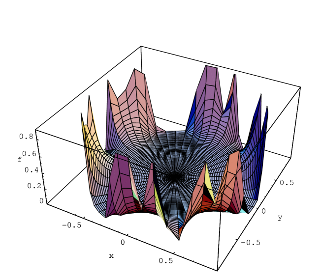
FIG. 12.: Relief of the function $g(r,\psi)$—see explanations in the text.

The gain of such representation becomes clear if we average the function $g(r,\psi)$ with respect to $\psi$. The numerical calculations give us:

$$\lim_{r\to 1}\left<g(r,\psi)\right>_{\psi}\equiv\lim_{r\to 1}\frac{1}{2\pi}\int_{0}^{2\pi}g(r,\psi)d\psi=\frac{\varpi}{(1-r^{2})^{2}}$$ (IV.31)

where $\varpi\simeq 0.0309$ (see the fig.(13)).

FIG. 13.: Plot of product $2\pi\left<g(r,\psi)\right>_{\psi}\times(1-r^{2})^{2}$ as a function of $r$.

Thus it is clear that for $r$ rather close to $1$ the diffusion is governed by the Laplacian on the surface of the constant negative curvature (the Lobachevskii plane). Representation of the Lobachevskii plane in the unit circle and in the upper half-plane (i.e. Poincare and Klein models) has been discussed in Section 2.4. Finally the diffusion equation (IV.26) takes the following form:

$$\frac{\partial}{\partial N}P(r,\psi,N)={\cal D}(1-r^{2})^{2}\Delta_{r,\psi}P(r,\psi,N)$$ (IV.32)

where $\displaystyle{\cal D}=\frac{a^{2}}{4\varpi c^{2}}$ is the ”diffusion coefficient” in the Lobachevskii plane and $N=L/a$ is the dimensionless chain length (i.e. effective number of steps).

Changing the variables $(r,\psi)\to(\mu,\psi)$, where $\displaystyle\mu=\ln\frac{1+r}{1-r}$, we get the unrestricted random walk on the 3-pseudosphere (see Eq.(III.58)). Correspondingly the distribution function $P(\mu,N)$ reads

$$P(\mu,N)=\frac{e^{-\frac{N{\cal D}}{4}}}{4\pi\sqrt{2\pi(N{\cal D})^{3}}}\int_{\mu}^{\infty}\frac{\xi\exp\left(-\frac{\xi^{2}}{4N{\cal D}}\right)}{\sqrt{\cosh\xi-\cosh\mu}}d\xi$$ (IV.33)

The physical meaning of the geodesics length on 3-pseudosphere, $\mu$, is straightforward: $\mu$ is the length of so-called ”primitive path” in the lattice of obstacles, i.e. length of the shortest path remaining after all topologically allowed contractions of the random trajectory in the lattice of obstacles. Hence, $\mu$ can be considered a nonabelian topological invariant, much more powerful than the Gauss linking number. This invariant is not complete except one point $\mu=0$ where it precisely classifies the trajectories belonging to the trivial homotopic class. Let us note that the length $\eta$ is proportional to the length of the primitive (irreducible) word written in terms of generators of the free group $\Gamma_{2}$.

V Physical applications. Polymer language in statistics of entangled chain–like objects

Topological constraints essentially modify the physical properties of statistical systems consisting of chain-like objects of completely different nature. It should be said that topological problems are widely investigated in connection with quantum field and string theories, 2D-gravitation, statistics of vortexes in superconductors and world lines of anyons, quantum Hall effect, thermodynamic properties of entangled polymers etc. Modern methods of theoretical physics allow us to describe rather comprehensively the effects of nonabelian statistics on physical behavior for each particular referred system; however, in our opinion, the following general questions remain obscure:

How does the changes in topological state of the system of entangled chain-like objects effect their physical properties?

How can the knowledge accrued in statistical topology be applied to the construction of the Ginzburg-Landau-type theory of fluctuating entangled chain-like objects?

In order to have representative and physically clear image for the system of fluctuating chains with the full range of nonabelian topological properties it appears quite natural to formulate general topological problems in terms of polymer physics. It allows us: to use a geometrically clear image of polymer with topological constraints as a model corresponding to the path integral formalism in the field theory; to advance in investigation of specific physical properties of biological and synthetical polymer systems where the topological constraints play a significant role.

For physicists the polymer objects are attractive due to many reasons. First of all, the adjoining of monomer units in chains essentially reduces all equilibrium and dynamic properties of the system under consideration. Moreover, due to that adjoining the behavior of polymers is determined by the space-time scales larger than for low-molecular-weight substances. The chain-like structure of macromolecules causes the following peculiarities (see, for instance, [73]): the so-called ”linear memory” (i.e. fixed position of each monomer unit along the chain); the low translational entropy (i.e. the restrictions on independent motion of monomer units due to the presence of bonds); large space fluctuations (i.e. just a single macromolecule can be regarded as a statistical system with many degrees of freedom).

It should be emphasized that the above mentioned ”linear memory” leads to the fact that different parts of polymer molecules fluctuating in space can not go one through another without the chain rupture. For the system of non-phantom closed chains this means that only those chain conformations are available which can be transformed continuously into one another, which inevitably give rise to the problem of knot entropy determination (see Section 2 for details).

A Polymer chain in 3D-array of obstacles

The 3D-model ”polymer chain in an array of obstacles” (PCAO) can be defined as follows ([49, 43, 66]). Suppose a polymer chain of length $L=Na$ is placed between the edges of the simple cubic lattice with the spacing $c$, where $N$ and $a$ are the number of monomer units in the chain and the length of the unit correspondingly. We assume that the chain cannot cross (”pass through”) any edges of the lattice.

The PCAO-model can be considered as the basis for a mean-field-like self-consistent approach to the major problem of entropy calculation of ensembles of strongly entangled fluctuating chains. Namely, choose the test chain, specify its topological state and assume that the lattice of obstacles models the effect of entanglements with the surrounding chains (”background”). Neglecting the fluctuations of the background and the topological constraints which the test chain produces for itself, we lose information about the correlations between the test chain and the background. However even in the simplest case we arrive at some nontrivial results concerning statistics of the test chain caused by topological interactions with the background. This means that for the investigation of properties of real polymer systems with topological constraints it is not enough to be able to calculate the statistical characteristics of chains in lattices of obstacles, but it is also necessary to be able to adjust any specific physical system to the unique lattice of obstacles, which is much more complicated task.

So, let us take a closed polymer chain without volume interactions (i.e. a chain with selfintersections) in the trivial topological state with respect to the 3D lattice of obstacles. It means that the chain trajectory can be continuously contracted to the point. It is clear that because of the obstacles, the macromolecule will adopt more compact conformation than the standard random walk without any topological constraints.

It is convenient to begin with the lattice realization of the problem. In this case the polymer chain can be represented as a closed $N$-step random walk on a cubic lattice with the length of elementary step $a$ being equal to the spacing of the array of obstacles, $c$. The general case $a\neq c$ will be considered later.

The random walk on a 3D-cubic lattice in the presence of the regular array of topological constraints produced by uncrossible strings on the dual lattice is equivalent to the free random walk on the graph—the Cayley tree with the branching number $z=6$.

The the average space dimension $R(N)\equiv\sqrt{R^{2}(N)}$ of the closed unentangled $N$-step random walk is ([43]):

$$R\sim aN^{1/4}$$ (V.1)

The outline of the derivation of the result (V.1) is as follows. First of all note that the Cayley tree with $z$ branches (called latter as $z$–tree with $z=2D$ branches) plays a role of the universal covering and is just a visualization of the free group $\Gamma_{\infty}$ with the infinite number of generators. At the same time $\Gamma_{\infty}/{\rm{\sf ZZ\hskip 1.70717pt}}^{D}=\Gamma_{z/2}$, where $Gamma_{z/2}$ is the free group with $z$ generators. Writing down the recursion relations for the probability $P(k,N)$ for the $N$-step random walk on the $z$-tree (compare to (III.24)–(III.53)), we can easily find the conditional limiting distribution for the function $\displaystyle P(k,m|N)=\frac{P(k,m)P(k,N-m)}{z(z-1)^{k-1}}$. Recall that $P(k,m|N)$ gives the conditional probability distribution of the fact that two sub-chains $C_{1}$ and $C_{2}$ of lengths $m$ and $N-m$ have the common primitive path $k$ under the condition that the composite chain $C_{1}\,C_{2}$ of length $N$ is closed and unentangled in regard to the obstacles;

$$P(k,m|N)\simeq\left(\frac{N}{2m(N-m)}\right)^{3/2}\,k^{2}\,\exp\left(-\frac{k^{2}N}{2m(N-m)}\right)$$ (V.2)

This equation enables us to get the following expressions for the mean length of the primitive path, $\left<k(m)\right>$ of closed unentangled $N$-link chain divided into two parts of the lengths $m$ and $N-m$ correspondingly

$$\left<k(m)\right>=\sum_{k=0}^{N}kP(k,m|N)\simeq\frac{2}{\sqrt{\pi}}\sqrt{\frac{2m(N-m)}{N}}\qquad(N\gg 1)$$ (V.3)

The primitive path itself can be considered a random walk in a 3D space with restriction that any step of the primitive path should not be strictly opposite to the previous one. Therefore the mean-square distance in the space $\left<({\bf r}_{0}-{\bf r}_{m})^{2}\right>$ between the ends of the primitive path of $k(m)$ steps is equal to

$$\left<({\bf r}_{0}-{\bf r}_{m})^{2}\right>=\frac{z}{z-2}ka^{2}$$ (V.4)

where ${\bf r}_{m}$ is the radius-vector of a link with the number $m$ and the boundary conditions are: ${\bf r}_{N}={\bf r}_{0}=0$. The mean-square gyration radius, $\left<R_{g}^{2}\right>$ of $N$-step closed unentangled random walk in the regular lattice of obstacles reads

$$\begin{array}[]{lllll}\left<R_{g}^{2}\right>&=&\displaystyle\frac{1}{2N^{2}}\sum_{n\neq m}\left<({\bf r}_{n}-{\bf r}_{m})^{2}\right>&=&\displaystyle\frac{1}{2N}\sum_{m=1}^{N}\left<({\bf r}_{0}-{\bf r}_{m})^{2}\right>\vskip 6.0pt plus 2.0pt minus 2.0pt\\ &&&=&\displaystyle\frac{z}{z-2}\frac{\sqrt{2\pi}}{8}a^{2}\sqrt{N}\end{array}$$ (V.5)

This result should be compared to the mean-square gyration radius of the closed chain without any topological constraints, $\left<R_{g,0}^{2}\right>=\frac{1}{12}a^{2}N$

The relation $R\sim N^{1/4}$ is reminiscent of the well-known expression for the dimension of randomly branched ideal macromolecule. The gyration radius of an ideal ”lattice animal” containing $N$ links is proportional to $N^{1/4}$. It means that both systems belong to the same universality class.

Now we turn to the mean-field calculation of the critical exponent $\nu$ of nonselfintersecting random walk in the regular lattice of obstacles [75]. Within the framework of Flory-type mean-field theory the nonequilibrium free energy, $F(R)$, of the polymer chain of size $R$ with volume interactions can be written as follows

$$F(R)=F_{\rm int}(R)+F_{\rm el}(R)$$ (V.6)

where $F_{\rm int}(R)$ is the energy of the chain self-interactions and $F_{\rm el}(R)$ is the ”elastic”, (i.e. pure entropic) contribution to the total free energy of the system. Minimizing $F(R)$ with respect to $R$ for fixed chain length, $L=Na$, we get the desired relation $R\sim N^{\nu}$.

Write the interacting part of the chain free energy written in the virial expansion

$$F_{\rm int}(R)=V\left(B\rho^{2}+C\rho^{3}\right)$$ (V.7)

where $V\sim R^{d}$ is the volume occupied by the chain in $d$-dimensional space; $\rho=\frac{N}{V}$ is the chain density; $B=b\frac{T-\theta}{\theta}$ and $C={\rm const}>0$ are the two– and three– body interaction constants respectively. In the case $B>0$ third virial coefficient contribution to Eq.(V.7) can be neglected [73].

The ”elastic” part of the free energy $F_{\rm el}(R)$ of an unentangled closed chain of size $R$ and length $Na$ in the lattice of obstacles can be estimated as follows

$$F_{\rm el}(R)={\rm const}+\ln P(R,m=N/2,N)={\rm const}+\ln\int dk\,P(k,N)\,P(R,k)$$ (V.8)

where the distribution function $P(k,m,N)$ is the same as in Eq.(V.2) and $P(R,k)$ gives the probability for the primitive path of length $k$ to have the space distance between the ends equal to $R$:

$$P(R,k)=\left(\frac{D}{2\pi ack}\right)^{d/2}\exp\left(-\frac{DR^{2}}{2ack}\right)$$ (V.9)

Substituting Eq.(V.8) for Eqs.(V.2) and (V.9) we get the following estimate

$$F_{\rm el}(R)=-\left(\frac{R^{4}}{a^{2}c^{2}N}\right)^{1/3}+o\left(R^{4/3}\right)$$ (V.10)

Equations (V.7) and (V.10) allow us to rewrite Eq.(V.6) in the form

$$F(R)\simeq B\frac{N^{2}}{R^{D}}-\left(\frac{R^{4}}{a^{2}c^{2}N}\right)^{1/3}$$ (V.11)

Minimization of Eq.(V.11) with respect to $R$ for fixed $N$ yields

$$R\sim B^{3/(4+3D)}(ac)^{2/(4+3D)}N^{\nu};\qquad\nu=\frac{7}{4+3D}$$ (V.12)

The upper critical dimension for that system is $D_{cr}=8$. For $D=3$ Eq.(V.12) gives

$$R\sim N^{7/13}$$ (V.13)

It is interesting to compare Eq.(V.12) to the critical exponent $\nu_{\rm an}$ of the lattice animal with excluded volume in the D–dimensional space, $\nu_{\rm an}=\frac{3}{4+D}$, which gives $\nu_{\rm an}=\frac{3}{7}$ for $D=3$. The difference in exponents signifies that the unentangled ring with volume interactions and the nonselfintersecting ”lattice animal” belong to different universality classes (despite in the absence of volume interactions they belong to the same class).

B Collapsed phase of unknotted polymer

In this Section we show which predictions about the fractal structure of a strongly collapsed phase of unknotted ring polymer can be made using the concept of ”polymer chain in array of obstacles”.

1 ”Crumpled globule” concept in statistics of strongly collapsed unknotted polymer loops

Take closed nonselfintersecting polymer chain of length $N$ in the trivial topological state . After a temperature decrease the formation of the collapsed globular structure becomes thermodynamically favorable [78]. Supposing that the globular state can be described in the virial expansion we introduce as usual two– and three–body interaction constants: $B=b\frac{T-\theta}{\theta}<0$ and $C={\rm const}>0$. But in addition to the standard volume interactions we would like to take into account the non-local topological constraints which obviously have a repulsive character. In this connection we express our main assertion [79].

The condition to form a trivial knot in a closed polymer changes significantly all thermodynamic properties of a macromolecule and leads to specific non-trivial fractal properties of a line representing the chain trajectory in a globule. We call such structure crumpled (fractal) globule. We prove this statement consistently describing the given crumpled structure and showing its stability.

It is well-known that in a poor solvent there exists some critical chain length, $g^{*}$, depending on the temperature and energy of volume interactions, so that chains which have length bigger than $g^{*}$ collapse. Taking long enough chain, we define these $g^{*}$-link parts as new block monomer units (crumples of minimal scale).

Consider now the part of a chain with several block monomers, i.e. crumples of smallest scale. This new part should again collapse in itself, i.e. should form the crumple of the next scale if other chain parts do not interfere with it. The chain of such new sub-blocks (crumples of new scale) collapses again and so on till the chain as a whole (see fig.14) forms the largest final crumple.

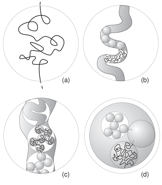
FIG. 14.: (a)–(c) Subsequent stages of collapse; (d) Self-similar structure of crumpled globule segregated on all scales.

Thus the procedure is completed when all initial links are united into one crumple of the largest scale. It should be noted that the line representing the chain trajectory obtained through the procedure described above resembles the 3D-analogue of the well known self-similar Peano curve.

The specific feature of the crumpled globule is in the fact that different chain parts are not entangled with each others, completely fill the allowed volume of space and are ”collapsed in themselves” starting from the characteristic scale $g^{*}$. It may seem that due to space fluctuations of the chain parts all that crumples could penetrate each others with the loops, destroying the self-similar scale-invariant structure described above. However it can be shown on the basis of PCAO–model that if the chain length in a crumple of an arbitrary scale exceeds $N_{e}$ then the crumples coming in contact do not mix with each other and remain segregated in space. Recall that $N_{e}$ is the characteristic distance between neighboring entanglements along the chain expressed in number of segments and, as a rule, the values of $N_{e}$ lie in the range $30\div 300$  [73].

Since the topological state of the chain part in each crumple is fixed and coincides with the state of the whole chain (which is trivial) this chain part can be regarded as an unknotted ring. Other chain parts (other crumples) function as effective lattice of obstacles surrounding the ”test” ring—see fig.15.

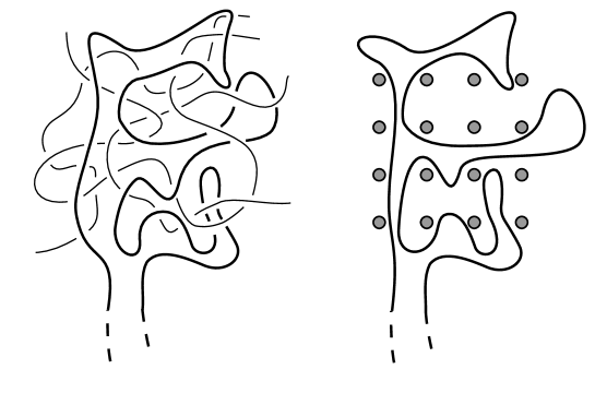
FIG. 15.: (a) Part of the closed unknotted chain surrounded by other parts of the same chain; (b) Unentangled ring in lattice of obstacles. The obstacles replace the effect of topological constraints produced by other part of the same chain.

Using the results of the Section 5.1 (see Eq.(V.5)) we conclude that any $M$-link ring subchain without volume interactions not entangled with any of obstacles has the size $R^{(0)}(M)\sim aM^{1/4}$. If $R^{(0)}$ is the size of an equilibrium chain part in the lattice of obstacles, the entropy loss for ring chain, $S$, as a function of its size, $R$, reaches its maximum for $R\simeq R^{(0)}$ (see Eq.V.10) and the chain swelling for values of $R$ exceeding $R^{(0)}(M)$ is entropically unfavorable. At the same time in the presence of excluded volume the following obvious inequality must be fulfilled $R(M)\sim aM^{1/3}$, which follows from the fact that density of the chain in the globular phase $\rho\sim R^{3}/N$ is constant. In connection with the obvious relation $R(M)>R^{(0)}(M)$ we conclude that the swelling of chains in crumples due to their mutual inter-penetration with the loops does not result in the entropy gain and, therefore, does not occur in the system with finite density. It means that the size of crumple on each scale is of order of its size in dense packing state and the crumples are mutually segregated in space. These questions are discussed in details in the work [79].

The system of densely packed globulized crumples corresponds to the chain with the fractal dimension $D_{f}=3$ ($D_{f}=3$ is realized from the minimal scale, $g^{*}$, up to the whole globule size). The value $g^{*}$ is of order

$$g^{*}=N_{e}(\rho a^{3})^{-2},$$ (V.14)

where $\rho$ is the globule density. This estimation was obtained in [79] using the following arguments: $g=(\rho a^{3})^{-2}$ is the mean length of the chain part between two neighboring (along the chain) contacts with other parts; consequently $N_{e}g$ is the mean length of the chain part between topological contacts (entanglements). Of course, as to the phantom chains, Gaussian blobs of size $g$ are strongly overlapped with others because pair contacts between monomers are screened (because of so-called $\theta$-conditions [78]). However for nonphantom chains these pair contacts are topologically essential because chain crossings are prohibited for any value and sign of the virial coefficient.

The entropy loss connected with the crumpled state formation can be estimated as follows:

$$S\simeq-\frac{N}{g^{*}}$$ (V.15)

Using Eq.(V.15) the corresponding crumpled globule density, $\rho$, can be obtained in the mean-field approximation via minimization of its free energy. The density of the crumpled state is less than that of usual equilibrium state what is connected with additional topological repulsive-type interactions between crumples:

$$\rho_{\rm crump}=\frac{\rho_{eq}}{1+{\rm const}(a^{6}/CN_{e})}<\rho_{\rm eq}$$ (V.16)

where $\rho_{\rm eq}$ is the density of the Lifshits’ globule.

The direct experimental verification of the proposed self-similar fractal structure of the unknotted ring polymer in the collapsed phase meets some technical difficulties. One of the ways to justify the ”crumpled globule” (CG) concept comes from its indirect manifestations in dynamic and static properties of different polymer systems. The following works should be mentioned in that context:

1. The two-stage dynamics of collapse of the macromolecule after abrupt changing of the solvent quality, found in recent light scattering experiments by B. Chu and Q. Ying (Stony Brook) [80].

2. The notion about the crumpled structure of the collapsed ring polymer allowed to explain [84] the experiments on compatibility enhancement in mixtures of ring and linear chains [85], as well as to construct the quantitative theory of a collapse of $N$–isopropilacrylamide gel in a poor water [83].

3. The paper [82] where the authors claim the observation of the crumpled globule in numerical simulations.

2 Knot Formation Probability

We can also utilize the CG-concept to estimate the trivial knot formation probability for dense phase of the polymer chain. Let us repeat that the main part of our modern knowledge about knot and link statistics has been obtained with the help of numerical simulations based on the exploiting of the algebraic knot invariants (Alexander, as a rule). Among the most important results we should mention the following ones:

– The probability of the chain self-knotting, $p(N)$, is determined as a function of chain length $N$ under the random chain closure [1, 86]. In the work [87] (see also the recent paper [88]) the simulation procedure was extended up to chains of order $N\simeq 2000$, where the exponential asymptotic of the type

$$p_{0}\sim\exp(-N/N_{0}(T))$$

has been found for trivial knot formation probability for chains in good and $\theta$-solvents. A statistical study of random knotting probability using the Vassiliev invariants has been undertaken in recent work [88].

– The knot formation probability $p$ is investigated as a function of swelling ratio $\alpha\;(\alpha<1)$ where $\displaystyle\alpha=\sqrt{\left<R_{g}^{2}\right>/\left<R_{g,0}^{2}\right>},\;\left<R_{g}^{2}\right>$ is the mean-square gyration radius of the closed chain and $\left<R_{g,0}^{2}\right>=\frac{1}{12}Na^{2}$ is the same for unperturbed $(\alpha=1)$ chain—see fig.16, where points correspond to the data of Ref.[1]; dashed line gives approximation in weak compression regime and solid line—the approximation based on the concept of crumpled globule.

FIG. 16.: Dependence of non-trivial knot formation probability, $p$ on swelling parameter, $\alpha$, in globular state.

It has been shown that this probability decreases sharply when a coil contracts from swollen state with $\alpha>1$ to the Gaussian one with $\alpha=1$  [89] and especially when it collapses to the globular state [1, 86].

– It has been established that in region $\alpha>1$ the topological constraints are screened by volume interactions almost completely [89].

– It has been shown that two unentangled chains (of the same length) even without volume interactions in the coil state repulse each other as impenetrable spheres with radius of order $\sqrt{\left<R_{g,0}^{2}\right>}$  [1, 90].

Return to fig.16, where the knot formation probability $p$ is plotted as a function of swelling ratio, $\alpha$, in the globular region $(\alpha<1)$. It can be seen that in compression region, especially for $\alpha<0.6$ data of numerical experiment are absent. It is difficult to discriminate between different knots in strongly compressed regime because it is necessary to calculate Alexander polynomial for each generated closed contour. It takes of order $O(l^{3})$ operations ($l$ is the number of self-interactions in the projection). This value becomes as larger as denser the system.

Let us present the theoretical estimations of the non-trivial knot formation probability $p(\alpha)$ in dense globular state $(\alpha<0.6)$ based on the CG-concept. The trivial knot formation probability under random linear chain closure, can be defined by the relation:

$$q(\alpha)=\frac{Z(\alpha)}{Z_{0}(\alpha)},\qquad q(\alpha)=1-p(\alpha)$$ (V.17)

where $Z(\alpha)$ is the partition function of unknotted closed chain with volume interactions for fixed value of swelling parameter, $\alpha$, and $Z_{0}(\alpha)$ is that of ”shadow” chain without topological constraints but with the same volume interactions. Both partition functions can be estimated within the framework of the mean field theory. To do so, let us write down the classic Flory-type representation for the free energy of the chain with given $\alpha$ (in equations below we suppose for the temperature $T\equiv 1$):

$$F(\alpha)=-\ln Z(\alpha)=F_{\rm int}(\alpha)+F_{\rm el}(\alpha)$$ (V.18)

where

$$F_{\rm el}(\alpha)=-S(\alpha)$$ (V.19)

Here the contributions $F_{\rm int}(\alpha)$ from the volume interactions to the free energies of unknotted and shadow chain of the same density (i.e. of the same $\alpha$) are equivalent. Therefore, the only difference concerns the elastic part of free energy, $F_{\rm el}$, or, in other words, the conformational entropy. Thus, the equation (V.17) can be represented in the form:

$$q(\alpha)=\exp\Bigl{(}-F(\alpha)-F_{0}(\alpha)\Bigr{)}=\exp\Bigl{(}S(\alpha)-S_{0}(\alpha)\Bigr{)}$$ (V.20)

According to Fixmann’s calculations [91] the entropy of phantom chain $S_{0}(\alpha)$ ($S_{0}(\alpha)=\ln Z_{0}(\alpha)$) in region $\alpha<1$ can be written in the following form:

$$S_{0}(\alpha)\simeq-\alpha^{-2}$$ (V.21)

In the weak compression region $0.6<\alpha\leq 1$ the probability of nontrivial knotting, $p(\alpha)$, can be estimated from the expression of the phantom ring entropy (Eq.(V.21)). The best fit of numerical data [1] gives us

$$p(\alpha)=1-A_{1}\exp\left(-B_{1}\alpha^{-2}\right)\qquad(0.6<\alpha\leq 1)$$ (V.22)

where $A_{1}$ and $B_{1}$ are the numerical constant.

The nontrivial part of our problem is reduced to the estimation of the entropy of strongly contracted closed unknotted ring $(\alpha\ll 1)$. Using Eqs.(V.14) and (V.15) and the definition of $\alpha$ we find

$$S(\alpha)\simeq-\frac{1}{N_{e}}\alpha^{-6}$$ (V.23)

In the region of our interest $(\alpha<0.6)$ the $\alpha^{-2}$-term can be neglected in comparison with $\alpha^{-6}$. Therefore, we the final probability estimate has the form:

$$p(\alpha)=1-A_{2}\exp\left(-\frac{1}{N_{e}}\alpha^{-6}\right)\qquad(\alpha<0.6)$$ (V.24)

where $A_{2}$ and $N_{e}$ are the numerical constants (their values are given below).

The probabilities of the nontrivial knot formation, $p(\alpha)$, in weak and strong compression regions are shown in fig.16 by the dotted and solid lines respectively. The values of the constants are: $A_{1}=1.2,\;B_{1}=0.25,\;A_{2}=0.925,\;N_{e}=34$; they are chosen by comparing Eqs.(V.22) and (V.24) with numerical data of Ref.[1].

3 Quasi-Knot Concept in Collapsed Phase of Unknotted Polymers

Speculations about the crumpled structure of strongly contracted closed polymer chains in the trivial topological state could be partially confirmed by the results of Chapters 1 and 2. The crucial question is: why the crumples remain segregated in a weakly knotted topological state on all scales in course of chain fluctuations. To clarify the point we begin by defining the topological state of a crumple, i.e. the unclosed part of the chain. Of course, mathematically strict definition of a knot can be formulated for closed (or infinite) contours exclusively. However the everyday experience tells us that even unclosed rope can be knotted. Thus, it seems attractive to construct a non-rigorous notion of a quasi-knot for description of long linear chains with free ends.

Such ideas were expressed first in 1973 by I.M. Lifshits and A.Yu. Grosberg [92] for the globular state of the chain. The main conjecture was rather simple: in the globular state the distance between the ends of the chain is of order $R\sim aN^{1/3}$, being much smaller than the chain contour length $L\sim Na$. Therefore, the topological state of closed loop, consisting of the chain backbone and the straight end-to-end segment, might roughly characterize the topological state of the chain on the whole. The composite loop should be regarded as a quasi-knot of the linear chain.

The topological state of a quasi-knot can be characterized by the knot complexity, $\eta$, introduced in Section 3 (see Eq.(III.15)). It should be noted that the quasi-knot concept failed for Gaussian chains where the large space fluctuations of the end-to-end distance lead to the indefiniteness of the quasi-topological state.

Our model of crumpled globule can be reformulated now in terms of quasi-knots. Consider the ensemble of all closed loops of length $L$ generated with the right measure in the globular phase. Let us extract from this ensemble the loops with $\eta(L)=0$ and find the mean quasi-knot complexity, $\left<\eta(l)\right>$, of an arbitrary subpart of length $l$ ($l/L=h=\mbox{const};\;0<h<1$) of the given loop. In the globular state the probability $\pi({\bf r})$ to find the end of the chain of length $L$ in some point ${\bf r}$ inside the globule of volume $R^{3}$ is of order $\displaystyle\pi({\bf r})\sim\frac{1}{R^{3}}$ being independent on ${\bf r}$ (this relation is valid when $La\gg R^{2}$). So, for the globular phase we could roughly suppose that the loops in the ensemble are generated with the uniform distribution. Thus our system satisfies the ”Brownian bridge” condition and according to conjecture of the Section 3 (Eq.(III.68) we can apply the following scale-invariant estimate for the averaged quasi-knot complexity $\sqrt{\left<\eta^{2}(l)\right>}$

$$\sqrt{\left<\eta^{2}(l)\right>}\sim l^{1/2}=h^{1/2}L^{1/2}$$ (V.25)

This value should be compared to averaged complexity $\sqrt{\left<\eta^{2}(l)\right>}$ of the part of the same length $l$ in the equilibrium globule created by an open chain of length $L$, i.e. without the Brownian bridge condition

$$\sqrt{\left<\eta^{2}(l)\right>}\sim l=hL$$ (V.26)

Comparing Eqs.(V.25) and (V.26) we conclude that any part of an unknotted chain in the globular state is far less knotted than the same part of an open chain in the equilibrium globule, which supports our mean-field consideration presented above. Let us stress that our statement is thermodynamically reliable and is independent of kinetics of crumpled globule formation.

VI Some ”tight” problems of the probability theory and statistical physics

Usually, in the conclusion it is accepted to overview the main results and imperceptibly prepare the reader to an idea how important the work itself is… We would not like go not by a usual way and to make a formal conclusion, because the summary of received results together with brief exposition of ideas and methods were indicated in the introduction and some incompleteness of account could only stimulate the fantasy of the reader.

On the contrary, we will try to pay attention to some hidden difficulties, which we permanently met on our way, as well as to formulate possible, yet unsolved problems, logically following from our consideration. Thus, we shall schematically designate borders of given research and shall allow the reader most to decide, whether a given subject deserves of further attention or not.

A Remarks and comments to the section 2

1. The derivation of Eqs.(II.59)–(II.60) assumed the passage from model with short–range interactions to the mean–field–theory, in which all spins are supposed to interact with each others. From the topological point of view such approximation is unphysical and requires the additional verification. We believe, that the considered model could be investigated with help of conformal theories and renormalisation group technique in the case of ”weak disorder”, i.e. when exists the strong asymmetry in choice of vertex crossings on a lattice.

2. As it was shown above, utilization of Jones topological invariant with necessity results in the study of thermodynamic properties of a Potts model. In the work [57] was mentioned, that Alexander polynomials are naturally connected to a partition function of a free fermion model and, hence, to an Ising model. Probably, the use of similar functional representation of Alexander polynomials in the frameworks of our disordered model would result in more simple equations, concerned with statistical properties of the Ising spin glasses.

3. All results received in this work are sticked to a model, which is effectively two–dimensional, since we are interested in statistical properties of a planar projection of knot in which all space degrees of freedom are thrown away and the topological disorder is kept only. Thus, physically, the model corresponds to the situation of a globular polymer chain located in a narrow two–dimensional slit. In connection with that the following question is of significant interest: how the space fluctuations of a trajectory in a three–dimensional space modify our consideration and, in particular, the answer (II.67)?

B Remarks and comments to sections 3 and 4

1. The investigation of topological properties of trajectories on multiconnected manifolds (on planes with sets removed points) from the point of view of the conformal field theory assumes a construction of topological invariants on the basis of monodromy properties of correlation functions of appropriate conformal theories. In connection with that there is a question concerning the possibility of construction of conformal theory with the monodromies of the locally–free group considered in work.

2. Without any doubts the question about the relation between topological invariants design and spectral properties of dynamic systems on hyperbolic manifolds is of extreme importance. The nature of mentioned connection consists in prospective dependence between knot invariants (in the simplest case, Alexander polynomials), recorded in the terms of a trace of products of elements of some hyperbolic group (see expression (III.14)) and trace formulae for some dynamic system on the same group.

3. Comparing distribution function of primitive paths $\mu$ (III.58) with the distribution function of a knot complexity of $\eta$ (III.15)), we can conclude that both these invariants have the same physical sense: a random walk in a covering space, constructed for lattice of obstacles, is equivalent from the topological point of view to a random walk on a Cayley tree. Thus, the knot complexity is proportional to a length of the primitive (irreducible) word, written in terms of group generators, i.e. is proportional to a geodesic length on some surface of constant negative curvature. We believe, that the detailed study of this interrelation will appear rather useful for utilization of algebraic invariants in the problems concerning statistics of ensembles of fluctuating molecules with a fixed topological state of each separate polymer chain.

3. Questions, considered in Section 3 admit an interpretation in spirit of spin glass theories, discussed at length of the Section 2. Let us assume, that there is a closed trajectory of length $L$, which we randomly drop on a plane with regular set of removed points. Let one point of a trajectory is fixed. The following question appears: what is a probability to find a random trajectory in a given topological state with respect to the set of removed points? The topological state of a trajectory is a typical example of the quenched disorder. According to the general concept, in order to find an appropriate distribution function (statistical sum), it is necessary to average the moments of topological invariant over a Gaussian distribution (i.e. with the measure of trajectories on a plane). The same assumptions are permitted us to assume, that the function $g(r,\psi)$ (Jacobian of conformal transformation)—see Fig.12 has a sense of an ultrametric ”potential”, in which the random walk takes place and where each valley corresponds to some given topological state of the path. The closer $r$ is to 1, the higher are the barriers between neighboring valleys. Thus, all reasonably long ($La\gg c^{2}$) random trajectories in such potential will become ”localized” in some strongly entangled state, in the sense that the probability of spontaneous disentanglement of a trajectory of length $La$ is of order of $\displaystyle\exp\left(-{\rm const}\frac{La}{c^{2}}\right)$. Probably this analogy could be useful in a usual theory of spin glasses because of the presence of explicit expression for the ultrametric Parisi phase space ([20]) in terms of a double-periodic analytic functions.

C Remarks and comments to section 5

1. We would like to express the conjecture (see also [93]) concerning the possibility of reformulation of some topological problems for strongly collapsed chains (see Section 5.4) in terms of integration over the set of trajectories with fixed fractal dimension but without any topological constraints.

We have argued that in ensemble of strongly contracted unknotted chains (paths) most of them have the fractal dimension $D_{f}=3$;

We believe that almost all paths in the ensemble of lines with fractal dimension $D_{f}=3$ are topologically isomorphic to simple enough (i.e. close to the trivial ) knot.

Let us remind, that the problem of the calculation of the partition function for closed polymer chain with topological constraints can be written as an integral over the set $\Omega$ of closed paths with fixed value of topological invariant (see Chapter 1):

$$Z=\int\limits_{\Omega}D_{w}\{r\}e^{-H}=\int\ldots\int D_{w}\{r\}e^{-H}\delta[I-I_{0}],$$ (VI.27)

where $D_{w}\{r\}$ means integration with the usual Wiener measure and $\delta[I-I_{0}]$ cuts the paths with fixed value of topological invariant ($I_{0}$ corresponding to the trivial knots).

If our conjecture is true, then the integration over $\Omega$ in Eq.(VI.27) for the chains in the globular phase (i.e. when $La\gg R^{2}$) can be replaced by the integration over all paths without any topological constraints, but with special new measure, $D_{f}\{r\}$:

$$Z=\int\ldots\int D_{f}\{r\}e^{-H}$$ (VI.28)

The usual Wiener measure $D_{w}\{r\}$ is concentrated on trajectories with the fractal dimension $D_{f}=2$. Instead of that, the measure $D_{f}\{r\}$ with the fractal dimension $D_{f}=3$ for description of statistics of unknotted rings should be used.

2. We believe, that the distribution of knot complexity found for some model systems can serve as a starting point in construction of a mean–field Ginsburg–Landau–type theory of fluctuating polymer chains with a fixed topology. From a physical point of view it seems to be important to rise the mean–field theory which takes into account the influence of topological restrictions on phase transitions in bunches of entangled directed polymers.

3. Let us note, that despite a number of experimental works, indirectly testifying for the existence of a fractal globule (see section 5 and references), the direct observation of this structure in real experiments is connected to significant technical difficulties and is so far not carried out. We believe, that the organization of an experiment on determination of a microstructure of an entangled ring molecule in a globular phase could introduce final clarity to a question on a crumpled globule existence.

REFERENCES

- [1] Vologodskii A V, Frank-Kamenetskii M D Usp. Fiz. Nauk 134 641 (1981) (in Russian); Vologodskii A V, Lukashin A V, Frank-Kamenetskii M D, Anshelevich V V Zh. Exp. Teor. Fiz. 66 2153 (1974); Vologodskii A V, Lukashin A V, Frank-Kamenetskii M D Zh. Exp. Teor. Fiz. 67 1875 (1974); Frank-Kamenetskii M D, Lukashin A V, Vologodskii A V Nature 258 398 (1975)
- [2] Wilsceck F Fractional Statistics and Anyon Superconductivity (Singapore: WSPC, 1990)
- [3] Majid S Int. J. Mod. Phys. A 8 4521 (1993)
- [4] Gómez C, Sierra G J. Math. Phys. 34 2119 (1993)
- [5] Jones V F R Pacific J. Math. 137 311 (1989); Likorish W B R Bull. London Math. Soc. 20 558 (1988); Wadati M, Deguchi T K, Akutsu Y Phys. Rep. 180 247 (1989)
- [6] Integrable Models and Strings Lect. Not. Phys. 436 (Springer: Heidelberg, 1994); Kauffman L H AMS Contemp. Math. Series 78 263 (1989)
- [7] Kauffman L H Topology 26 395 (1987)
- [8] Vassiliev V A Complements of Discriminants of Smooth Maps: Topology and Applications Math. Monographs 98 (Trans. AMS, 1992); Bar-Natan D preprint Harvard, 1992
- [9] Edwards S F Proc. Roy. Soc. 91 513 (1967)
- [10] Yor M J. Appl. Prob. 29 202 (1992); Math. Finance 3 231 (1993)
- [11] Comtet A, Desbois J, Monthus C J. Stat. Phys. 73 433 (1993); Desbois J J.Phys. A 25L-195, L-755 (1992); Desbois J, Comtet A J.Phys. A 25 3097 (1992)
- [12] Wiegel F Introduction to Path-Integrals Methods in Physics and Polymer Science (Singapore: WSPC, 1986)
- [13] Khandekar D S, Wiegel F J. Phys. A 21 L-563 (1988); J. Phys. (Paris) 50 2205 (1989)
- [14] Hofstadter D Phys. Rev. B 14 2239 (1976); Guillement J, Helffer B, Treton P J. Phys. (Paris) 50 2019 (1989)
- [15] Wiegmann P B, Zabrodin A V Phys. Rev. Lett. 72 1890 (1994); Nucl. Phys. B 422 [FS] 495 (1994)
- [16] Bellissard J Lect. Notes Phys. 257 99 (1986)
- [17] Dubrovin B A, Novikov S P, Fomenko A T, Modern Geometry (Moscow: Nauka, 1979)
- [18] Wu F Y Rev. Mod. Phys. 54 235 (1982)
- [19] Baxter R J Exactly Solvable Models in Statistical Mechanics (London: Academic Press, 1982)
- [20] Mezard M, Parisi G, Virasoro M Spin Glass Theory and Beyond (Singapore: WSPC, 1987)
- [21] Lifshits I M, Gredeskul S A, Pastur L A Introduction to the theory of disordered systems (Moscow: Nauka, 1982)
- [22] Reidemeister K Knotentheorie (Berlin: Springer, 1932)
- [23] Kauffman L H Knots and Physics (Singapore: WSPC, 1991)
- [24] Grosberg A Yu, Nechaev S J. Phys. A 25 4659 (1992)
- [25] Wu F Y J. Knot Theory Ramific. 1 32 (1992)
- [26] Grosberg A Yu, Nechaev S Europhys. Lett. 20 613 (1992)
- [27] Duplantier B, David F J. Stat. Phys. 51 327 (1988)
- [28] Edwards S F, Anderson P W J. Phys. F 5 965 (1975)
- [29] Cwilich G, Kirkpatrick T R J. Phys. A 22 4971 (1989)
- [30] De Santis E, Parisi G, Ritort F, preprint: cond-mat/9410093
- [31] Gross D J, Kanter I, Sompolinsky H Phys. Rev. Lett. 55 304 (1985)
- [32] Bellissard J, Simon B J. Funct. Anal. 48 408 (1982)
- [33] Gutzwiller M Chaos in Classical and Quantum Mechanics (Heidelberg: Springer, 1990)
- [34] Terras A Harmonic Analysis on Symmetric Spaces and Applications (Berlin: Springer, 1979)
- [35] Hejhal D The Selberg Trace Formula for Lect. Notes in Math. 548 (Berlin: Springer, 1976); 1001 (Berlin: Springer, 1983)
- [36] Chassaing P, Letac G, Mora M Probability Measures on Groups Lect. Not. Math. 1064 (1983)
- [37] Nechaev S K, Statistics of Knots and Entangled Random Walks (Singapore: WSPC, 1996)
- [38] Lerda A Anyons Lect. Notes in Phys. 14 (Berlin: Springer, 1992)
- [39] Fürstenberg H Trans. Am. Math. Soc 198 377 (1963); Tutubalin V Prob. Theor. Appl. (in Russian) 10 15 (1965)
- [40] Nechaev S, Sinai Ya Bol. Sci. Bras. Mat. 21 121 (1991)
- [41] Koralov L, Nechaev S, Sinai Ya Prob. Theor. Appl. 38 331 (1993)
- [42] Mirlin A, Fyodorov Y J. Phys. A 24 227 (1991); Fyodorov Y Basic Features of Efetov’s supersymmetry approach Mesoscopic Quantum Physics, Les Houches, session LXI, 1994 (Amstredam: Elsevier, 1995)
- [43] Khokhlov A, Nechaev S Phys. Lett. A 112 156 (1985); Nechaev S, Semenov A, Koleva M Physica, A 140 506 (1987)
- [44] Nechaev S, Vershik A J. Phys. A 27 2289 (1994)
- [45] Monastyrsky M, Nechaev S Mod. Phys. Lett. A (1997)
- [46] Nechaev S, Grosberg A Yu, Vershik A M J. Phys. A 29 2411 (1996)
- [47] Kesten H Trans. Amer. Math. Soc. 92 336 (1959)
- [48] Vershik A M Topics in Algebra 26, pt.2 467 (1990), (Warszawa: Banach Center Publication, PWN Publ.); Proc. Am. Math. Soc. 148 1 (1991)
- [49] Helfand E, Pearson D S J. Chem. Phys. 79 2054 (1983); Rubinstein M, Helfand E J. Chem. Phys. 82 2477 (1985)
- [50] Cates M E, Deutsch J M J. Phys. (Paris) 47 2121 (1986)
- [51] Vershik A M private communication
- [52] Desbois J, Nechaev S J. Stat. Phys. 88 201 (1997)
- [53] Comtet A, Nechaev S, J. Phys. A, 31 2767 (1998)
- [54] Desbois J, Nechaev S J. Phys. A, 31 5609 (1998)
- [55] Jones W F R Bull. Am. Math. Soc. 12 103 (1985)
- [56] Vershik A M, Kerov S Dokl. Ac. Nauk SSSR 301 777 (1988) (In Russian)
- [57] Kauffman L H, Saleur H Comm. Math. Phys. 141 293 (1991)
- [58] Akutsu Y, Deguchi T K Phys. Rev. Lett. 67 777 (1991); Akutsu Y, Wadati M J. Phys. Soc. Jap. 56 (1987)
- [59] Birman J Knots, Links and Mapping Class Groups Ann. Math. Stud. 82 (Princeton: Princeton Univ. Press, NJ, 1976)
- [60] Mumford M Tata Lectures on Theta, I, II Progress in Mathematics 28, 34 (Boston, MA: Birkhauser, 1983)
- [61] Letchikov Russian Math. Surveys 51 49 (1996)
- [62] Zinn-Justin J Quantum Field Theory and Critical Phenomena (Oxford: Clarendon, 1989)
- [63] Gerzenshtein M E, Vasiljev V B Prob. Theor. Appl. 4 424 (1959) (in Russian); Karpelevich F I, Tutubalin V N, Shour M G Prob. Theor. Appll. 4 432 (1959) (in Russian)
- [64] Polyakov A M Mod. Phys. Lett. A 3 325 (1988); Witten E Comm. Math. Phys. 121 351 (1989)
- [65] Belavin A A, Polyakov A M, Zamolodchikov A B Nucl. Phys. B 241 333 (1984)
- [66] Nechaev S K J.Phys. A 21 3659 (1988)
- [67] Ito K, McKean H P Diffusion Processes and Their Sample Paths (Berlin: Springer, 1965)
- [68] Golubev V V Lectures on analytic theory of differential equations (Moscow: GITTL, 1950); Venkov A B, preprint LOMI P/2/86
- [69] Dotsenko Vl S Nucl. Phys. B 235 [FS11] 54 (1984)
- [70] Knizhnik V G, Zamolodchikov A B Nucl. Phys. B 247 83 (1984)
- [71] Guadarini E, Martinelli M, Mintchev M CERN-TH preprints 5419/89, 5420/89, 5479/89
- [72] Chandrassekharan K Elliptic Functions ( Berlin: Springer, 1985)
- [73] Grosberg A Yu, Khokhlov A R Statistical physics of macromolecules (Moscow: Nauka, 1993)
- [74] Koralov L B, Nechaev S K, Sinai Ya G Chaos 1 131 (1991)
- [75] Gutin A M, Grosberg A Yu, Shakhnovich E I Macromolecules 26 1293 (1993)
- [76] De Gennes P G Scaling Concepts in Polymer Physics (Ithaca: Cornell Univ. Press, 1979)
- [77] Kholodenko A private communications
- [78] Lifshits I M, Grosberg A Yu, Khokhlov A R Rev. Mod. Phys. 50 683 (1978)
- [79] Grosberg A Yu, Nechaev S K, Shakhnovich E I J. Phys. (Paris) 49 2095 (1988)
- [80] Chu B, Ying Q, Grosberg A Macromolecules 28 180 (1995)
- [81] Grosberg A, Rabin Y, Havlin S, Neer A Europhys. Lett. 23 373 (1993); Grosberg A, Rabin Y, Havlin S, Neer A Biofizika 38 75 (1993)
- [82] Ma J, Straub J E, Shakhnovich E I J. Chem. Phys. 103 2615 (1995)
- [83] Grosberg A Yu, Nechaev S K Macromolecules 24 2789 (1991)
- [84] Khokhlov A R, Nechaev S K J.Phys II (Paris) 6 1547 (1996)
- [85] Nachlis W L, Kambour R P, McKnight W J Abstracts of the 35th IUPAC Congress 2 796; Nachlis W L, Kambour R P, McKnight W J Polymer 39 3643 (1994)
- [86] Mishels J P, Wiegel F W Proc. Roy. Soc. A 403 269 (1986)
- [87] Koniaris K, Muthukumar M Phys. Rev. Lett. 66 2211 (1991)
- [88] Tsurusaki K, Deguchi T J. Phys. Soc. Jap. 64 1506 (1995); Deguchi T, Tsurusaki K J. Knot Theory Ramific. 3 321 (1994)
- [89] Klenin K V, Vologodskii A V, Anshelevich V V, Dykhne A M J. Biomol. Struct. Dyn. 5 1173 (1988)
- [90] Van Rensburg E J, Whittington S G J.Phys. A 23 3573 (1990); Le Bret M Biopolymers 19 619 (1980)
- [91] Fixmann M J. Chem. Phys. 36 306 (1962)
- [92] Lifshits I M, Grosberg A Yu Zh. Exp. Teor. Fiz. 65 2399 (1973)
- [93] Grosberg A Yu, Nechaev S K Adv. Polym. Sci. 106 1 (1993)