A first principle computation of the thermodynamics of glasses

Abstract

We propose a first principle computation of the equilibrium thermodynamics of simple fragile glasses starting from the two body interatomic potential. A replica formulation translates this problem into that of a gas of interacting molecules, each molecule being built of $m$ atoms, and having a gyration radius (related to the cage size) which vanishes at zero temperature.

We use a small cage expansion, valid at low temperatures, which allows to compute the cage size, the specific heat (which follows the Dulong and Petit law), and the configurational entropy.

1 Introduction

Take a three dimensional classical system consisting of many particles, interacting through a short range potential with a repulsive core. Very often this system will undergo, upon cooling or upon compression, a solidification into an amorphous solid state - the glass state. The conditions required for observing this glass phase is the avoidance of crystallisation, which can always be obtained through a fast enough quench (the meaning of ’fast’ depends very much of the type of system) [1]. There also exist potentials which naturally present some kind of frustration with respect to the crystalline structure. Whether their actual stable state is a crystal or a glass is not known, but they are known to solidify into glass states, even when cooled slowly - such is the case for instance of binary mixtures of hard spheres, soft spheres, or Lennard-Jones particles with appropriately different radii. These have been studied a lot in recent numerical simulations [2, 3, 4, 5, 6].

Our aim is to compute the equilibrium thermodynamic properties of this glass phase, using the statistical mechanical approach, namely starting from the microscopic Hamiltonian (an attempt to build up a non equilibrium thermodynamic phenomenology can be found in [7]). We shall therefore assume that crystallisation has been avoided, and consider only the amorphous solid state. The general framework of our approach finds its roots in old ideas of Kauzman [8], Adam and Gibbs [9], which received a boost when Kirkpatrick, Thirumalai and Wolynes underlined the analogy between structural glasses and some generalized spin glasses [11]. This framework should provide a good description of fragile glass-formers. These are the systems in which the increase of relaxation time upon decreasing the temperature is much faster than Arrhenius- often parametrized as a Vogel-Fulcher law, displaying a divergence of the relaxation time at a finite temperature[1]. In this approach the glass transition, measured from dynamical effects, is supposed to be associated with an underlying thermodynamic transition at the Kauzman or Vogel-Fulcher temperature $T_{K}$. This ideal glass transition is the one which should be observed on infinitely long time scales in fragile glass-formers[1]. This transition is of an unusual type, since it presents two apparently contradictory features:

1. The transition is continuous (second order) from the thermodynamical point of view: the internal energy is continuous, and the transition is signalled by a discontinuity of the specific heat which jumps from its liquid value above $T_{K}$ to a value very close to that of a crystal phase below.

2. The order parameter is discontinuous at the transition.

In order to make this last statement precise we shall have to define an order parameter for the glass phase in the framework of equilibrium statistical mechanics, which involves some subtleties and will be addressed below. At this introductory stage let us take loosely as an order parameter the correlation in the positions of the particles at very large times. In the liquid there is no correlation. In the glass the positions are correlated in time. Clearly the order parameter jumps discontinuously between the liquid phase and the glass phase. The two properties above are indeed observed in generalized spin glasses [12]. The problem of the existence or not of a diverging correlation length is still an open one [13].

This analogy is suggestive, but it also hides some very basic differences, like the fact that spin glasses have quenched disorder while structural glasses do not. The recent discovery of some generalized spin glass systems without quenched disorder [14, 15, 16] has given credit to the idea that this analogy is not fortuitous. The problem was to turn this general idea into a consistent computational scheme allowing for some quantitative predictions. Important steps in this direction were invented in [17, 18], which showed how useful it is to study several coupled copies of the same system in order to characterize properly the glass phase. In a previous preliminary study, we used some of these ideas to estimate the glass temperature, arriving from the liquid phase [19]. However the approximations we did were not adequate for the description of the low temperature phase. Here we concentrate instead on the properties of the glass phase itself and we introduce approximations which are much more appropriate to describe its properties particularly at low temperatures. We are now able to construct analytical tools for doing computations in the glass phase and to test the results in numerical (and eventually real) experiments. A brief description of a part of the present work has appeared in [20].

In the next section we shall present in more details the general physical picture underlying our approach. In sect.3 we shall explain why and how one can characterize and study the glass phase using a replicated liquid. Sect. 4 derives the Hamiltonian of the molecular liquid, which is studied in the next two sections, first of all by a small cage expansion in sect.5, then by a molecular HNC closure in sect.6. In sect.7 we present the results of these various approximations concerning the glass transition temperature and the thermodynamic quantities. Sect. 8 gives a list of some directions into which this work could be extended. Two appendices contain the derivation of the molecular HNC closure on one hand, and its expansion to second order in the small cage parameter on the other hand.

2 The basic scenario

In this section we want to present some of the general ideas which provide a background to our approach. These have to do with the existence of a configurational entropy, and the identification of the glass transition as a point where the configurational entropy vanishes. These ideas are presented in general, without special reference to a specific system. They can be derived in great details in some mean field spin glass models. Although the microscopic description of these models is somewhat remote from the actual glass problem which interests us, we have included for completeness a short summary of some of the results found in these systems. This will help to formulate the basic hypotheses of our approach.

2.1 Configurational entropy

We consider a system of $N$ particles moving in a volume $V$ of a d-dimensional space, and interacting by some short range potential. These could be for instance hard spheres or Lennard-Jones particles.

Let us introduce the free energy functional $F[\rho]$ which depends on the local particle density $\rho(x)$ and on the temperature. We suppose that at sufficiently low temperature this functional has an exponentially large number of minima [21]. More precisely, the number of free energy minima with free energy density $f=F/N$ is supposed to be exponentially large in some region of free energies, $f_{min}(T)<f<f_{max}(T)$:

$${\cal N}(f,T,N)\approx\exp(NS_{c}(f,T))\ .$$ (1)

Exactly at zero temperature these minima coincide with the mimima of the potential energy as function of the coordinates of the particles. The function $S_{c}$ is called the complexity or the configurational entropy (it is the contribution to the entropy coming from the existence of an exponentially large number of locally stable configurations). The number of local minima is supposed to vanish outside of the region $f_{min}(T)<f<f_{max}(T)$, and the configurational entropy $S_{c}(f,T)$ is supposed to go to zero continuously at $f_{min}(T)$, as found in all existing models so far (see fig.1).

Figure 1: Qualitative shape of the configurational entropy versus free energy. The whole curve depends on the temperature. The saddle point which dominates the partition function, for $m$ constrained replicas, is the point $f^{*}$ such that the slope of the curve equals $m/T$ (for the usual unreplicated system, $m=1$). If the temperature is small enough the saddle point sticks to the minimum $f=f_{min}$ and the system is in its glass phase.

Let us first discuss the properties of the system at thermal equilibrium: we thus consider the case where each configuration of the system is assigned a probability given by its Boltzmann weight. We label the free energy minima by an index $\alpha$. To each of them we can associate a free energy $F_{\alpha}$ and a free energy density $f_{\alpha}=F_{\alpha}/N$. In the low temperature region we suppose that the total free energy of the system ($\Phi$) can be well approximated by the sum of the contributions to the free energy of each particular minimum:

$$Z\equiv\exp(-\beta N\Phi)\simeq\sum_{\alpha}\exp(-\beta Nf_{\alpha}).$$ (2)

For large values of $N$ we can write

$$\exp(-N\beta\Phi)\approx\int_{f_{min}}^{f_{max}}df\exp[-N(\beta f-S_{c}(f,T))]\ .$$ (3)

We can thus use the saddle point method and approximate the integral with the integrand evaluated at its maximum. We find that

$$\Phi=\min_{f}\Phi(f)\equiv f^{*}-TS_{c}(f^{*},T),$$ (4)

where

$$\Phi(f)\equiv f-TS_{c}(f,T).$$ (5)

This formula is quite similar to the usual formula for the free energy ,i.e. $f=\min_{E}(E-TS(E))$, where $S(E)$ is the entropy density as a function of the energy density ($E$). The main difference is the fact that the total entropy of the system has been decomposed into the contribution due to small fluctuations around a given configuration (this piece has been included into $f$), and the contribution due to the existence of a large number of locally stable configurations, the configurational entropy.

Calling $f^{*}$ the value of $f$ which minimize $\Phi(f)$, we have two possibilities:

• The minimum lies inside the interval and it can be found as the solution of the equation $\beta=\partial S_{c}/\partial f$. In this case we have

  $$\Phi=f^{*}-TS_{c}^{*},\ \ \ S_{c}^{*}=S_{c}(f^{*},T).$$ (6)

  The system may stay in one of the many possible minima. The number of accessible minima is $\exp(NS_{c}^{*})$ . The entropy of the system is thus the sum of the entropy of a typical minimum and of $S_{c}^{*}$, which is the contribution to the entropy coming from the exponentially large number of metastable configurations.

• The minimum is at the extreme value of the range of variability of $f$: it sticks at $f^{*}=f_{min}$ and the total free energy is $\Phi=f_{min}$. In this case the contribution of the configurational entropy to the free energy is zero. The different states which contribute to the free energy have a difference in free energy density which is of order $N^{-1}$ (a difference in total free energy of order 1). This situation is often encountered in spin glasses, both in usual cases of spin glasses with quenched disorder [22, 23], and also in some spin glass systems without quenched disorder [14, 15, 16].

One aim of the theory of glasses at equilibrium could be to demonstrate from first principles the existence of a configurational entropy function such as depicted in fig. 1, and to compute it. This is difficult to achieve. For instance Kepler’s conjecture, a simple zero temperature statement saying that there is no denser packing of hard spheres in three dimensions than the fcc lattice, has resisted a proof for more than three centuries [24]. Here we shall take a more modest starting point: we shall assume the existence of the local minima and of the configurational entropy function with the general properties depicted above, and within this assumption we shall show how to compute (approximately but with a rather good accuracy, and one which can be improved systematically) the various properties of the system, including the configurational entropy function itself.

2.2 Mean field situation

So far, the only systems for which the above program could be carried out in all details are some type of mean field spin glasses with a discontinuous jump of the order parameter at the transition [12, 11, 25, 26, 27, 28].

Although we will not need all the ingredients that have been found in these other problems, it is useful to recall some of them; later on we will mention how this picture might be modified in a realistic - non mean field - system. The configurational entropy function is convex, and previous work indicates that it depends smoothly on the temperature, the main effect of a temperature change being a global shift of the free energies. Starting from high temperatures, we thus encounter the following temperature regions (we use here the language of liquids and glasses).

• For $T>T_{D}$ the free energy functional is dominated by the uniform density solution, $\rho(x)=\rho$ (there may exist close to $T_{D}$ other minima [29, 26], but their total contribution has a higher free energy than the uniform solution). The system is obviously in the fluid phase.

• In the region where $T_{D}>T>T_{K}$, the minimum of the function $\Phi(f)$ is within the interval $[f_{min}(T),f_{max}(T)]$. Therefore the system can stay in one of many different states. The entropy of the equilibrium system receives a contribution from the configurational entropy, which is non zero. A very surprising result, found in all generalized mean field spin glasses with discontinuous transition so far, is that the total free energy of the system including the configurational entropy contribution, $\Phi(f^{*})$, is equal to the free energy of the fluid solution with uniform $\rho$ [17, 18]. This result has not received a general explanation beyond the simple idea of the transition at $T_{D}$ being a fragmentation of accessible phase space into many separated pockets, the total volume of which should be continuous at $T_{D}$. Although the thermodynamics is still given by the usual expressions of the liquid phase and the free energy is analytic at $T_{D}$, below this temperature the system, at each given moment of time, may stay in one of the exponentially large number of minima.

• In the region where $T<T_{K}$ the saddle point of $\Phi$ sticks at its minimum and the free energy is dominated by the contribution of a few minima having the lowest possible value $f_{min}(T)$. Here the free energy is no more the analytic continuation of the free energy in the fluid phase. A phase transition is present at $T_{K}$ and the specific heat is discontinuous here.

The intermediate phase $T_{D}>T>T_{K}$ is particularly interesting. In the mean field systems, an exact solution of the Langevin dynamics indicates a dynamical phase transition at $T_{D}$, the system being trapped in some states with a free energy which is extensively higher than that of the equilibrium state [30]. For the realistic finite dimensional problems which we want to study, the situation is much less clear, but one can speculate that the system will equilibrate in this regime, very slowly [11]. The time to jump from one minimum to another minimum is quite large: it is an activated process which is controlled by the height of the barriers which separate the different minima. The correlation time will become very large below $T_{D}$ and for this reason $T_{D}$ is called the dynamical transition point. The correlation time (which should be proportional to the viscosity) diverges only at the true thermodynamic transition temperature, sometimes called the ideal glass temperature $T_{K}$ (see fig.2). The precise form of this divergence is not well understood. It is natural to suppose that one should get a divergence of the form $\exp(A/(T-T_{K})^{\nu})$ for an appropriate value of $\nu$, but a reliable analytic computation of $\nu$ is lacking [11, 31]. Experiments can often be fitted by this law with various values of $\nu$, including the Vogel-Fulcher fit with $\nu=1$. The equilibrium configurational entropy is different from zero (and it is a number of order 1) when the temperature is smaller than $T_{D}$, it decreases with the temperature and it vanishes linearly at $T=T_{K}$. At this temperature the entropy of a single minimum becomes equal to the total entropy and the contribution of the configurational entropy to the total free energy vanishes. Therefore the total entropy and the internal energy are continuous at the transition.

Figure 2: Relaxation time vs temperature in discontinuous spin-glasses. The right hand curve is the mean-field prediction, which gives a dynamical transition at a temperature $T_{D}$ above the static transition temperature $T_{K}$. The left curve is a conjecture on the behaviour in finite dimensional systems: activated processes smear the dynamic transition. The relaxation time diverges only at the static temperature $T_{K}$, but becomes experimentally large already around the glass temperature $T_{g}$.

2.3 Relationship to experiments

The above scenario is appealing in that it puts into a unified framework a number of experimental facts on glasses, as well as some general theoretical ideas.

Experimentally, the system falls out of equilibrium when its relaxation time becomes larger than the experimental time. The ‘glass transition temperature’, defined conventionally as the temperature where the typical relaxation time reaches a value of order one hour, falls somewhere between $T_{K}$ and $T_{D}$. By considering slower and slower quenches, one can equilibrate the system at lower temperatures. However in this scenario there exists an underlying thermodynamic transition at the temperature $T_{K}$, which is the ideal glass transition temperature. This temperature is also the one where the viscosity would diverge in the Vogel-Fulcher type fitting of the viscosity versus temperature. Clearly it also corresponds to the Kauzman temperature: the excess entropy of the supercooled liquid with respect to the crystal is basically equal to the configurational entropy, which vanishes precisely at $T_{K}$. The experimental fact that the Kauzman temperature and the Vogel-Fulcher one are close to each other has been noted many times, and is also found in the Adam-Gibbs relation [9].

The dynamical temperature $T_{D}$ also receives a natural interpretation. In mean field, therefore neglecting activated processes, the relaxation time diverges with a power law at $T_{D}$, and the autocorrelation function develops an infinitely long plateau. This slowing down is described precisely by the mode coupling theory [10]. In the mean field approximation the height of the barriers separating the different minima is infinite and the temperature $T_{D}$ is sharply defined as the point where the correlation time diverges. In the real world activated process (which are neglected in the mean field approximation and consequently in the mode coupling theory) have the effect of producing a finite (but large) correlation time also at and below $T_{D}$ (the precise meaning of the dynamical temperature beyond mean field approximation is not so clear -see [5]; probably the best definition is that $T_{D}$ is the temperature where the mode-coupling theory predicts a transition). Therefore one expects that the mode coupling description will give good results in the region largely above $T_{D}$, a fact that has been checked accurately in experiments [32] and numerical simulations[33].

A last point which is predicted within the basic scenario, and has been checked numerically, is a specific type of aging and modification of the fluctuation-dissipation relation. The aging behaviour, which has been seen many years ago already in some polymeric glasses [34], can be studied in details in spin glasses [35]. These studies, initiated by the work of Cugliandolo and Kurchan [30], have led to some well defined generalisation of the basic equilibrium properties such as time translation invariance and fluctuation-dissipation theorem (FDT). This generalisation is not limited to the narrow scope of some special mean field spin-glasses, but seems to provide a general description of glassy dynamics in many systems, including structural glasses. The modification of the fluctuation-dissipation relation can be measured directly, although the experiments are not simple. On the other hand, numerical simulations for a binary mixture of soft spheres [2] or Lennard-Jones particles [4] have found exactly the non-trivial modification which is predicted by the general scenario, providing therefore a confirmation of its validity at least on their (limited) time scales.

3 A static order parameter for the glass phase

In this section we wish to explain the general strategy for describing and computing properties of an amorphous solid state. We are particularly interested in systems with many metastable states, having a non zero configurational entropy. We shall explain the general strategy trying to keep away as much as possible from any specific model, the more precise formulation for our problem will be given in the next section. Let us consider a system of $N$ particles, interacting by a two body potential with a Hamiltonian

$$H=\sum_{1\leq i\leq j\leq N}v(x_{i}-x_{j})$$ (7)

where the particles move in a volume $V$ of a d-dimensional space, and $v$ is an arbitrary short range potential with a short range repulsion, like a $1/r^{12}$ potential or a Lennard-Jones one. We shall take the thermodynamic limit $N,V\to\infty$ at fixed density $\rho=N/V$. For simplicity, we do not consider here the description of mixtures of different types of particles. The generalization to mixtures is necessary if one wants to compare more precisely to simulations, which are performed on mixtures in order to avoid crystallisation. This generalization, together with a detailed comparison, will be presented in a forthcoming paper [40]. Some general background is provided by the review paper [35].

3.1 Time persistent correlations

Before going to a purely static description of the order parameter, let us first discuss a dynamical one. At an atomic level one often tends to associate the glass transition with the divergence of the time scale on which a labelled particle can get out of its trap. While this is an intuitive picture, it is not possible to translate it into a good definition of the solid phase: because of the excitation and movements of vacancies and other defects, this individual trapping time scale is always finite, although it will increase exponentially when the temperature gets small. In order to get a proper definition of the solid, it has been proposed [41, 42] to use a generalisation of the Edwards Anderson order parameter of the type:

$$Q_{EA}(p)=\lim_{t\to\infty}\lim_{N\to\infty}{1\over N}\sum_{jk}\langle e^{ip\cdot(x_{j}(0)-x_{k}(t))}\rangle$$ (8)

where $p$ is an arbitrary non zero wave vector, the order of magnitude of which is one over the typical interparticle distance. When the system is in the liquid phase the above order parameter is zero and when it is in the glass phase this order parameter is non zero (even in the presence of single particle diffusion).

This definition would hold for the equilibrium dynamics, i.e. assuming that the system is in equilibrium at time $t=0$. As we know the glass never reaches equilibrium and therefore it ages: correlations are not stationary in time. The proper generalization of the previous correlation taking into account the aging effect takes the slightly more complicated form (where the order of limits is crucial):

$$Q_{EA}(p)=\lim_{\tau\to\infty}\lim_{t_{w}\to\infty}\lim_{N\to\infty}{1\over N}\sum_{jk}\langle e^{ip\cdot(x_{j}(t_{w})-x_{k}(t_{w}+\tau))}\rangle$$ (9)

This gives a sensible dynamical definition of the glass phase.

3.2 Correlations between two copies

We would like a purely static description of the solid phase in the framework of equilibrium statistical mechanics, in a case where there are no Bragg peaks. As soon as we have a solid phase the translational symmetry is broken and the system can be in many states. For crystalline order these many states just differ from each other by rotations or translations which can be easily taken care of by appropriate boundary terms. In the glass case, in order to choose a state, one should first know the average position of each atom in the solid, which requires an infinite amount of information. Had we known this information, we could have added to the Hamiltonian an infinitesimal but extensive pinning field which attracts each particle to its equilibrium position, sending $N$ to infinity first, before taking the limit of zero pinning field. This is the usual way of identifying the phase transition.

In order to get around the problem of the description of the amorphous solid phase, a simple method has been developed in the spin glass context. Pictorially, one could say that although we do not know the conjugate field, the system itself knows it. The idea, borrowed from spin glass theory [43, 44], is then to consider two copies of the system, with an infinitesimal extensive attraction. One then identifies the transition temperature from the fact that the two replicas remain close to each other in the limit of vanishing coupling (having sent $N$ to infinity first).

In the case of glasses we can thus consider two identical systems of particles, $\{x_{j}\}$ and $\{y_{j}\}$, with a total energy function:

$$E=\sum_{1\leq i\leq j\leq N}(v(x_{i}-x_{j})+v(y_{i}-y_{j}))+\epsilon\sum_{i,j}w(x_{i}-y_{j})$$ (10)

where we have introduced a small attractive potential $w(r)$ between the two systems. The precise shape of $w$ is irrelevant, insofar as we shall be interested in the limit $\epsilon\to 0$, but its range should be of order or smaller than the typical interparticle distance. The order parameter is then the correlation function between the two systems:

$$g_{xy}(r)=\lim_{\epsilon\to 0}\lim_{N\to\infty}{1\over\rho N}\sum_{ij}<\delta(x_{i}-y_{j}-r)>$$ (11)

In the liquid phase this correlation function is identically equal to one, while it has a nontrivial structure in the glass phase, reminiscent of the pair correlation of a dense liquid, but with an extra peak around $r\simeq 0$. Let us notice that we expect a discontinuous jump of this order parameter at the transition, in spite of its being second order in the thermodynamic sense. The existence of a non trivial order parameter is associated with the spontaneous breaking of a symmetry: For $\epsilon=0$, with periodic boundary conditions, the system is symmetric under a global translation of the $x$ particles with respect to the $y$ particles. This symmetry is spontaneously broken in the low temperature phase, where the particles of each subsystem tend to sit in front of each other. One could equally use the Fourier transform of this cross-correlation, which then gives back, but in an equilibrium framework, the Edwards Anderson order parameter defined in (9).

3.3 Thermodynamics below $T_{K}$: replicas

The previous method is a reasonable definition of an equilibrium order parameter which can be used in simulations or in analytic studies in order to identify the phase transition arriving from the liquid phase. However this technique can be improved in order to study quantitatively the glass phase itself.

Let us assume that in the glass phase there exists a non zero configurational entropy, as introduced above. Clearly the knowledge of this configurational entropy as a function of free-energy and temperature, $S_{c}(f,T)$, will allow us to reconstruct all the interesting thermodynamic properties of the system. It has been realised by Monasson[17] that the configurational entropy can be reconstructed from a study of an arbitrary number, $m$, of copies of the system, when they are constrained to be in the same state. As we will need to analytically continue the results in $m$, we shall call the copies ’replicas’. An alternative and related method is to introduce a real coupling of the system to another system which is thermalized[18]; this has been used recently in order to study the glass phase [5, 45]. The formulation which we present here is slightly different from, but equivalent to, that of [17].

The basic idea is extremely simple. Instead of two copies of the system, let us consider $m$ copies which are constrained to stay in the same minimum. We shall discuss below how one can achieve this constraint, but let us first discuss the physics of this constrained system. Its partition function is:

$$Z_{m}=\int_{f_{m}}^{f_{M}}df\ e^{-N[m\beta f-S_{c}(f,T)]}$$ (12)

The dependence on the number $m$ of replicas of the total free energy,

$$\Phi(m,T)=-{1\over\beta N}\log Z_{m}\approx\min_{f}(m\ f-TS_{c}(f,T))\ ,$$ (13)

allows to compute the configurational entropy $S_{c}(f,T)$ as a function of the free energy, using:

$${\partial\Phi(m,T)\over\partial m} = f$$

$${m^{2}\over T}{\partial\phi(m,T)\over\partial m} = S_{c}\ ,$$ (14)

where $\phi(m,T)$ is the free energy per particle:

$$\phi(m,T)={\Phi(m,T)\over m}\ .$$ (15)

If the glass transition is due to the entropy crisis described in the previous section (and this is our main hypothesis), then the crucial quantity is the value of the slope $s_{0}(T)$ of the configurational entropy at the lowest free energy:

$$s_{0}(T)\equiv{\partial S_{c}\over\partial f}(f_{0}(T))$$ (16)

The usual glass transition is determined by $T_{K}s_{0}(T_{K})=1$. For the replicated and constrained system, the phase transition temperature $T^{(m)}$ depends on the number $m$ of replicas and is determined by (see fig. 1):

$$T^{(m)}s_{0}(T^{(m)})=m$$ (17)

It is very natural to assume that $s_{0}(T)$ is a smooth function of temperature, going to a constant at zero temperature (we shall check this hypothesis self-consistently later). Then we see that, when $m$ is continued analytically to real values, smaller than unity, one can have $T^{(m)}<T_{K}$. The replicated and constrained system can thus be in the liquid phase for temperatures smaller than the glass transition temperature $T_{K}=T^{(1)}$: it is then made up of molecules, each of which contains one atom of each replica, but these molecules are in a liquid state. The basic reason for this crucial fact is that for $m<1$ the effective interaction potential (assuming for simplicity molecules of very small radius) is decreased from $v(r)$ to $mv(r)$, thus displacing the glass transition to lower temperatures.

Figure 3: A sketch of the typical phase diagram in the temperature-$m$ plane, for a system with $m$ weakly coupled replicas. In the whole high temperature region above the full line the system is in a liquid phase. There are two liquid phases, above the horizontal line $T=T_{K}$ the various replicas are not correlated in the limit of the coupling $\epsilon$ going to zero. On the contrary the liquid state at $m<1$, in the region between the full line and the dashed line, is a molecular liquid where the various replicas form molecular bound states. The low temperature region below the full line (characterized by $m=m^{*}(T)$) is the glass phase. In this glass phase, for a given temperature, the free energy per replica is $m$ independent. Therefore one can deduce the free energy of the glass ( with $m<1$ and $T<T_{K}$) from the knowledge of the free energy in the molecular liquid.

We are interested in the free energy in the glass phase, therefore in the region $m=1$ and $T<T_{K}$. This free energy cannot be computed from that of the liquid with $m=1$, $T>T_{K}$ because of the phase transition at $T_{K}$. However we shall now show that one can deduce it from the free energy of the molecular fluid at $m<1$. This molecular fluid with $m<1$ has a transition to a glass state at the temperature $T=T^{(m)}<T_{K}$. Inside the glass phase, thus for $T<T^{(m)}$, the free energy of the replicated and constrained system is given by the condition

$$S_{c}(f,T)=0$$ (18)

and it is independent on $m$.

Let us now look at the phase diagram at a fixed temperature $T<T_{K}$, varying $m$ (see fig. 3). The free energy per particle $\phi(m,T)$ of the molecular liquid is an increasing function of $m$ at small $m$, which reaches a maximum at a point $m^{*}<1$ where the glass transition takes place (obviously $m^{*}$ is the solution of: $T\;s_{0}(T)=m^{*}$). As the free energy in the glass phase is $m$ independent, the liquid free energy at the transition $\phi(m^{*},T)$ (which is equal to the glass free energy at the transition) is equal, for $T<T_{K}$, to the free energy $\phi(m=1,T)$ of the glass at the temperature $T$. We have thus shown that the knowledge of the free energy of the molecular liquid, $\phi(m,T)$, allows to compute the free energy of the glass.

These basic observations are at the heart of our strategy for computing properties of the glass phase. We shall write down more explicit formulas in our case below. We would like first to make three comments on this approach:

• For $T<T_{K}$ and $m>m^{*}$, the free energy $\phi(m)$ is constant and larger than the analytic continuation of the free energy $\phi(m)$ of the molecular liquid. If one would have followed this molecular liquid in the region $m>m^{*}$, one would have found that $\partial\phi/\partial m<0$, predicting a negative configurational entropy. Instead, the glass transition occurs and the configurational entropy sticks to zero in the whole glass phase. The fact that the free energy in the glass phase is larger than the analytic continuation from the high temperature phase explains why the specific heat has a discontinuity downward when we decrease the temperature. This is in variance with what happens generally in other transitions (at least in the mean field approximation) where the free energy in the low temperature phase is smaller than the analytic continuation from the high temperature phase and the specific heat has a discontinuity upward when we decrease the temperature.

• In practice in order to try to constrain the systems to be in the same state, one introduces some small attractive coupling, of order $\epsilon$, between the replicas. It is thus important to understand when this coupling leads to a molecular liquid. The phase diagram shown in fig.3 can be conjectured from the following elementary study of the free energy, confirmed by exact computations of mean field discontinuous spin glasses [26, 18, 5, 28]. There are a priori four possible cases. If the $m$ replicas are in the same state, the free energy is $\Phi=\min_{f}(m\ f-TS_{c}(f,T))-m(m-1)\epsilon$. If they are in different states, the free energy is $\Phi=m\min_{f}(\ f-TS_{c}(f,T))$. On top of this, the free energy minimum can either stick to $f_{0}$ (glass phase) or be at a value $f$ larger than $f_{0}$ (liquid). One just needs to find out which situation actually minimizes the free energy, for given values of $m$ and $T$. The solution is displayed in fig.3, showing that there is an intermediate molecular liquid phase at $m<1$.

• The ’replicas’ which we introduce here play a slightly different role compared to the ones used in disordered systems: there is no quenched disorder here, and no need to average a logarithm of the partition function. ‘Replicas’ are introduced to handle the problem of the absence of description of the amorphous state. We do not know of any other procedure to characterize an amorphous solid state in the framework of equilibrium statistical mechanics. There is no ‘zero replica’ limit, but there is, as in disordered systems, an analytic continuation in the number of replicas. We shall see that this continuation looks rather innocuous.

4 The replica approach to structural glasses: general formalism

In this section we write down the formulas corresponding to the replica approach introduced in the previous section. We keep here to the case of simple glass formers consisting of $N$ particles interacting by a pair potential $v(r)$ in a space of dimension $d$.

4.1 The partition function

The usual partition function, used e.g. in the liquid phase, is

$$Z_{1}\equiv{1\over N!}\int\prod_{i=1}^{N}(d^{d}x_{i})\ e^{-\beta H}$$ (19)

We wish to study the transition to the glass phase through the onset of an off-diagonal correlation in replica space. We use $m$ replicas and introduce the Hamiltonian of the replicated system:

$$H_{m}=\sum_{1\leq i<j\leq N}\sum_{a=1}^{m}v(x^{a}_{i}-x^{a}_{j})+\sum_{j_{1}...j_{m}\in\{1,...,N\}}W(x^{1}_{j_{1}},...,x^{m}_{j_{m}})$$ (20)

where $W$ is an attractive interaction. The precise form of $W$ is unimportant: it should be a short range attraction respecting the replica permutation symmetry, and its strength which will be sent to zero in the end. For instance one could take

$$W(r^{1},...,r^{m})=\epsilon\sum_{1\leq a<b\leq m}w(r^{a}-r^{b})$$ (21)

with $w(r)$ a smooth short range two body attraction.

The partition function of the replicated system is

$$Z_{m}\equiv{1\over N!^{m}}\int\prod_{i=1}^{N}\prod_{a=1}^{m}(d^{d}x^{a}_{i})\ e^{-\beta H_{m}}$$ (22)

The order parameter is the generalised cross correlation:

$$\rho(r^{1},...,r^{m})={1\over N}\sum_{j_{1}...j_{m}}<\delta(x_{j_{1}}^{1}-r^{1})...\delta(x_{j_{m}}^{m}-r^{m})>$$ (23)

where the average is the Boltzmann-Gibbs average with the measure proportional to $\exp(-\beta H_{m})$.

4.2 Molecular bound states

At low enough temperature, we expect that the particles in the different replicas will stay close to each other due to the joint effect of the small inter-replica attraction and the intra-replica interactions: when the system is in the glass phase, the role of the attractive term $W$ will be to insure that all replicas fall into the same glass state, so that the particles in different replicas stay at the same place, apart from some thermal fluctuations: A vanishingly small interaction between replicas will give rise to a strong correlation. As the thermal fluctuations are relatively small throughout the solid phase (one can see this for instance from the Lindeman criterion), one can identify the molecules and relabel all the particles in the various replicas in such a way that the particle $j$ in replica $a$ always stays close to particle $j$ in replica $b$. All the other relabelings are equivalent to this one, producing a global factor $N!^{m-1}$ in the partition function.

We therefore need to study a system of molecules, each of them consisting of $m$ atoms (one atom from each replica). It is natural to write the partition function in terms of the variables $r_{i}$ which describe the centers of masses of the molecules, and the relative coordinates $u_{i}^{a}$, with $x_{i}^{a}=r_{i}+u_{i}^{a}$ and $\sum_{a}u_{i}^{a}=0$:

$$Z_{m} = {1\over N!}\int\prod_{i=1}^{N}\left(d^{d}r_{i}\right)\prod_{i=1}^{N}\prod_{a=1}^{m}(d^{d}u_{i}^{a})\prod_{i=1}^{N}\left(m^{d}\delta(\sum_{a}u_{i}^{a})\right)$$ (24)

$$\exp\left(-\beta\sum_{i<j,a}v(r_{i}-r_{j}+u^{a}_{i}-u^{a}_{j})-\beta\sum_{i}W(u^{1}_{i},...,u^{m}_{i})\right)$$

5 The small cage expansion

In order to transform these ideas into a tool for doing explicit computations of the thermodynamic properties of a glass we have to use an explicit method for computing the free energy as function of the temperature and $m$. As is usually the case, in the liquid phase exact analytic computations are not possible and we have to do some approximations. In this section we shall use the fact that the thermal fluctuations of the particles in the glass are small at low enough temperature: the size of the ‘cage’ seen by each particle is therefore small, allowing for a systematic expansion. What we will be describing here are the thermal fluctuations around the minimum of the potential of each particle, in the spirit of the Einstein model for vibrations of a crystal.

5.1 Legendre transform

We start from the replicated partition function $Z_{m}$ described in molecular coordinates in (24). Assuming that the relative coordinates $u^{a}_{i}$ are small, we can expand $W$ to leading order and write:

$$Z_{m} = {1\over N!}\int\prod_{i=1}^{N}\left(d^{d}r_{i}\right)\prod_{i=1}^{N}\prod_{a=1}^{m}(d^{d}u_{i}^{a})\prod_{i=1}^{N}\left(m^{d}\delta(\sum_{a}u_{i}^{a})\right)$$ (25)

$$\exp\left(-\beta\sum_{i<j,a}v(r_{i}-r_{j}+u^{a}_{i}-u^{a}_{j})-{1\over 4\alpha}\sum_{i}\sum_{a,b}(u^{a}_{i}-u^{b}_{i})^{2}\right)$$

In the end we are interested in the limit $(1/\alpha)\to 0$. We would like first to define the size $A$ of the molecular bound state, which is also a measure of the size of the cage seen by each atom in the glass, by:

$${\partial\log Z_{m}\over\partial(1/\alpha)}\equiv{m(1-m)\over 2}dNA=-{1\over 4}\sum_{i}\sum_{a,b}\langle(u_{i}^{a}-u_{i}^{b})^{2}\rangle$$ (26)

(d is the dimension, N is the number of particles). We Legendre transform the free energy $\phi(m,\alpha)=-(T/m)\log Z_{m}$, introducing the thermodynamic potential per particle $\psi(m,A)$:

$$\psi(m,A)=\phi(m,\alpha)+Td{(1-m)\over 2}{A\over\alpha}$$ (27)

What we want to see is whether there exists a minimum of $\psi$ at a finite value of $A$.

At low temperatures, this minimum should be at small $A$, and so we shall seek an expansion of $\psi$ in powers of $A$. It turns out that this can be found by an expansion of $\phi$ in powers of $\alpha$, used as an intermediate bookkeeping in order to generate the low temperature expansion. This may look confusing since we are eventually going to send $\alpha$ to $\infty$. However this method is nothing but a usual low temperature expansion in the presence of an infinitesimal breaking field. For instance if one wants to compute the low temperature expansion of the magnetization in a $d$-dimensional Ising model in an infinitesimal positive magnetic field $h$, the main point is that the magnetisation is close to one. One can organise the expansion by studying first the case of a large magnetic field, performing the expansion in powers of $\exp(-2h)$, and in the end letting $h\to 0$. A little thought shows that the intermediate -large $h$- expansion is just a bookkeeping device to keep the leading terms in the low temperature expansion. What we do here is exactly similar, the role of $h$ being played by $1/\alpha$.

5.2 Zeroth order term

We use the equivalent form:

$$Z_{m}(\alpha)={1\over N!}\int\prod_{i=1}^{N}\prod_{a=1}^{m}(d^{d}u_{i}^{a})\prod_{i}{d^{d}X_{i}\over\sqrt{2\pi\alpha\over m^{2}}^{d}}\exp\left(-\beta\sum_{i<j,a}v(x_{i}^{a}-x_{j}^{a})-{m\over 2\alpha}\sum_{i,a}(x_{i}^{a}-X_{i})^{2}\right)\ .$$ (28)

For $\alpha\to 0$, the identity

$$\exp\left(-{m\over 2\alpha}(x_{i}^{a}-X_{i})^{2}\right)\simeq\left({2\pi\alpha\over m}\right)^{d/2}\delta^{d}(x_{i}^{a}-X_{i})$$ (29)

gives:

$$Z_{m}^{0}(\alpha)=\left({2\pi\alpha\over m}\right)^{dNm/2}\left({2\pi\alpha\over m^{2}}\right)^{-dN/2}{1\over N!}\int\prod_{i}dX_{i}\exp\left(-\beta m\sum_{i<j}v(X_{i}-X_{j})\right)\ .$$ (30)

In this expression we recognise the integral over the $X_{i}$’s as the partition function $Z_{liq}(T^{*})$ of the liquid at the effective temperature $T^{*}$, defined by

$$T^{*}\equiv T/m\ .$$ (31)

Therefore the free energy, at this leading order, can be written as:

$${\beta\phi^{0}(m,\alpha)}={d(1-m)\over 2m}\log{2\pi\alpha\over m}-{d\over 2m}\log(m)-{1\over mN}\log Z_{liq}(T^{*})$$ (32)

5.3 First order term

In order to expand to next order, we start from the representation (25) and expand the interaction term to quadratic order in the relative coordinates:

$$Z_{m} = \int\prod d^{d}r_{i}d^{d}u_{i}^{a}\prod_{i}\left(m^{d}\delta(\sum_{a}u_{i}^{a})\right)\exp\left(-\beta m\sum_{i<j}v(r_{i}-r_{j})\right)$$

$$\exp\left(-{\beta\over 2}\sum_{i<j}\sum_{a\mu\nu}(u_{i}^{a}-u_{j}^{a})^{\mu}(u_{i}^{a}-u_{j}^{a})^{\nu}\partial_{\mu}\partial_{\nu}v(r_{i}-r_{j})-{1\over 4\alpha}\sum_{a,b}(u_{i}^{a}-u_{i}^{b})^{2}\right)\ .$$

(The indices $\mu$ and $\nu$, running from $1$ to $d$, denote space directions). Notice that in order to carry this step, we need to assume that the interaction potential $v(r)$ is smooth enough, excluding hard cores. To expand at small $\alpha$ we need the properties of the set of $m$ random variables $u^{a}$ living on one site with measure $P(u)\propto\delta(\sum_{a}u^{a})\exp(-(1/4\alpha)\sum_{ab}(u^{a}-u^{b})^{2})$. It turns out that these are gaussian random variables with a first moment which vanishes and a second moment which is equal to:

$$\langle u^{a}_{\mu}u^{b}_{\nu}\rangle_{0}=\left(\delta^{ab}-{1\over m}\right){\alpha\over m}\delta_{\mu\nu}\ .$$ (33)

Expanding (5.3) to first order in $\alpha$ we have:

$$\log Z_{m}=\log Z_{m}^{0}-{\beta\over 2}\sum_{i<j}\sum_{a\mu\nu}\langle(u_{i}^{a}-u_{j}^{a})^{\mu}(u_{i}^{a}-u_{j}^{a})^{\nu}\rangle_{0}\langle\partial_{\mu}\partial_{\nu}v(r_{i}-r_{j})\rangle^{*}$$ (34)

where the average $\langle.\rangle_{0}$ is that for the $u$ variables with the gaussian measure (33), and the average $\langle.\rangle^{*}$ is over the center of mass positions $r_{i}$, which are those of a liquid phase thermalized at the temperature $T^{*}=T/m$.

The free energy to first order is equal to:

$${\beta\phi(m,\alpha)}={d(m-1)\over 2m}\log{1\over\alpha}-\alpha\beta C+{d(1-m)\over 2m}\log{2\pi\over m}-{d\over 2m}\log{m}-{1\over mN}\log Z_{liq}(T^{*})$$ (35)

where the constant $C$ is proportional to the expectation value of the Laplacian of the potential, in the liquid phase at the temperature $T^{*}$:

$$C\equiv{1\over 2}{1-m\over m^{2}}\sum_{j(\neq i)}\langle\Delta v(z_{i}-z_{j})\rangle^{*}$$ (36)

Differentiation with respect to ${1\over\alpha}$ gives the size of the cage:

$${\beta}{\partial\phi\over\partial(1/\alpha)}=-{(1-m)\over 2m}d\alpha+\alpha^{2}\beta C=-{(1-m)\over 2}dA$$ (37)

Expanding this equation in perturbation theory in $A$ we have:

$$\alpha=mA-{2\beta m^{3}C\over d(m-1)}A^{2}$$ (38)

The Legendre transform is then easily expanded to first order in $A$:

$${\beta\psi(m,A)} = {\beta\phi}(m,\alpha)+d{(1-m)\over 2}{A\over\alpha}$$ (39)

$$= {d(1-m)\over 2m}\log(2\pi A)-\beta mAC+{d(1-m)\over 2m}-{d\over 2m}\log m-{1\over mN}\log Z_{liq}(T^{*})$$

This very simple expression gives the free energy as a function of the number of replicas, $m$, and the cage size $A$. We need to study it at $m\leq 1$, where we should maximise it with respect to $A$ and $m$. The fact that we seek a maximum when $m<1$ instead of the usual procedure of minimising the free energy is a well established fact of the replica method, appearing as soon as the number of replicas is less than $1$ [22].

As a function of $A$ , the thermodynamic potential $\psi$ has a maximum at:

$$A=A_{max}\equiv{d(1-m)\over 2\beta m^{2}}{1\over C}={d\over\beta}{1\over\int d^{d}rg^{*}(r)\Delta v(r)}$$ (40)

where $g^{*}$ is the pair correlation of the liquid at the temperature $T^{*}$. A study of the potential $\psi(m,A_{max})$, which equals $\phi(m)$, as a function of $m$ then allows to find all the thermodynamic properties which we seek, using the formulas of the previous section. This step and the results will be explained below in sect. 7, where we shall also compare the results to those of other approximations.

5.4 Higher order

The systematic expansion of the thermodynamic potential $\psi$ in powers of $A$ can be carried out easily to higher orders. However the result involves some more detailed properties of the liquid at the effective temperature $T^{*}$. For instance at second order one needs to know not only the free energy and pair-correlation of the liquid at temperature $T^{*}$, but also the three points correlation. It is certainly interesting to try to push this expansion further, taking the information on the liquid at temperature $T^{*}$ from some numerical simulations. In this paper we have decided to stay within some relatively simple schemes which require only the knowledge of the pair-correlation $g^{*}(r)$. Therefore we shall not pursue this higher order expansion here, leaving it for future work.

5.5 Harmonic resummation

One can obtain a partial resummation of the small cage expansion described above by integrating exactly over the relative vibration modes of the molecules. We shall use such a procedure here, which is a kind of harmonic expansion in the solid phase.

We work directly with $1/\alpha=0$ and start from the replicated partition function (5.3), within the quadratic expansion of the interaction potential $v$ in the relative coordinates $u_{i}^{a}$. (Clearly it is assumed that the $1/\alpha\to 0^{+}$ limit has been taken, and that its effect is to build up molecular bound states). The exact integration over the gaussian relative variables gives:

$$Z_{m}={m^{Nd/2}\sqrt{2\pi}^{Nd(m-1)}\over N!}\int\prod_{i=1}^{N}d^{d}r_{i}\exp\left(-\beta m\sum_{i<j}v(r_{i}-r_{j})-{m-1\over 2}Tr\log\left(\beta M\right)\right)$$ (41)

where the matrix $M$, of dimension $Nd\times Nd$, is given by:

$$M_{(i\mu)(j\nu)}=\delta_{ij}\sum_{k}v_{\mu\nu}(r_{i}-r_{k})-v_{\mu\nu}(r_{i}-r_{j})$$ (42)

and $v_{\mu\nu}(r)=\partial^{2}v/\partial r_{\mu}\partial r_{\nu}$. We have thus found an effective Hamiltonian for the centers of masses $r_{i}$ of the molecules, which basically looks like the original problem at the effective temperature $T^{*}=T/m$, complicated by the contribution of vibration modes which give the ‘Trace Log’ term. We expect that this should be a rather good approximation for the glass phase. Unfortunately, even within this approximation, we have not been able to compute the partition function exactly. The density of eigenstates of the matrix $M$ is a rather complicated object and we have developed a simple approximation scheme in order to estimate it.

We thus proceed by using a ’quenched approximation’, i.e. neglecting the feedback of vibration modes onto the centers of masses. This approximation becomes exact close to the Kauzman temperature where $m\to 1$. The free energy is then:

$${\beta\phi(m,T)}=-{d\over 2m}\log(m)-{d(m-1)\over 2m}\log(2\pi)-{1\over mN}\log Z(T^{*})+{m-1\over 2m}\langle Tr\log\left(\beta M\right)\rangle^{*}$$ (43)

which involves again the free energy and correlations of the liquid at the temperature $T^{*}$. Computing the spectrum of $M$ is an interesting problem of random matrix theory, in a subtle case where the matrix elements are correlated. Some efforts have been devoted to such computations in the liquid phase where the eigenmodes are called instantaneous normal modes [49]. It might be possible to extend these approaches to our case. Here we shall rather propose a simple resummation scheme which should be reasonable at high densities-low temperatures.

Considering first the diagonal elements of $M$, we notice that in this high density regime there are many neighbours to each point, and thus a good approximation is to neglect the fluctuations of these diagonal terms and substitute them by their average value. We thus write:

$$\sum_{k}v_{\mu\nu}(r_{i}-r_{k})\simeq\delta_{\mu\nu}{1\over d}\int d^{d}rg^{*}(r)\Delta v(r)\equiv r_{0}$$ (44)

Here and in what follows, we have not written explicitly the density. We choose to work with density unity in order to simplify the formulae: this value can always be obtained by using an appropriate scale of length. In the approximation (44) the diagonal matrix elements are all equal and can be factorized, leading to:

$$\langle Tr\log\left(\beta M\right)\rangle^{*}=Nd\log(\beta r_{0})+\langle Tr\log\left(\delta_{ij}\delta_{\mu\nu}-{1\over r_{0}}v_{\mu\nu}(r_{i}-r_{k})\right)\rangle^{*}$$ (45)

This form lends itself to a perturbative expansion in powers of $1/r_{0}$. The computation of the $p$-th order term in this expansion,

$${\cal T}_{p}\equiv{(-1)^{p-1}\ overpr_{0}^{p}}\langle\sum_{{i_{1}...i_{p}}\atop{\mu_{1}...\mu_{p}}}v_{\mu_{1}\mu_{2}}(r_{i_{1}}-r_{i_{2}})...v_{\mu_{p-1}\mu_{p}}(r_{i_{p-1}}-r_{i_{p}})v_{\mu_{p}\mu_{1}}(r_{i_{p}}-r_{i_{1}})$$ (46)

still involves the $p$-th order correlation functions of the liquid at $T^{*}$. We have approximated this full correlation by introducing a simple ‘chain’ approximation involving only the pair correlation. This chain approximation consists in replacing, for $p>2$, the full correlation by a product of pair correlations. It selects those contributions which survive in the high density limit; systematic corrections could probably be computed in the framework of the approach of [50], we leave this for future work. Within the chain approximation, ${\cal T}_{p}$ is approximated by:

$${\cal T}_{p} = \sum_{\mu_{1}...\mu_{p}}\int dx_{1}...dx_{p}\ g^{*}(x_{1},....,x_{p})\ [v_{\mu_{1}\mu_{2}}(x_{1}-x_{2})...v_{\mu_{p-1}\mu_{p}}(x_{p-1}-x_{p})v_{\mu_{p}\mu_{1}}(x_{p}-x_{1})]$$ (47)

$$\simeq\sum_{\mu_{1}...\mu_{p}}\int dx_{1}...dx_{p}\ [g^{*}(x_{1}-x_{2})v_{\mu_{1}\mu_{2}}(x_{1}-x_{2})]...[g^{*}(x_{p}-x_{1})v_{\mu_{p}\mu_{1}}(x_{p}-x_{1})]\ .$$

In this last form we need to compute a convolution which can be factorised through the introduction of the Fourier transform of the pair correlation function. We thus introduce the Fourier transformed functions $a$ and $b$ which are defined from the pair correlation $g^{*}(r)$ by:

$$\int d^{d}r\ g^{*}(r)v_{\mu\nu}(r)e^{ikr}\equiv\delta_{\mu\nu}\ a(k)+\left({k_{\mu}k_{\nu}\over k^{2}}-{1\over d}\delta_{\mu\nu}\right)b(k)\ .$$ (48)

In terms of these Fourier transforms, the $p$-th order term in the $1/r_{0}$ expansion is simply

$${\cal T}_{p}=\int{d^{d}k\over(2\pi)^{3}}\left(a(k)+{d-1\over d}b(k)\right)^{p}+(d-1)\int{d^{d}k\over(2\pi)^{3}}\left(a(k)-{1\over d}\ .b(k)\right)^{p}\ ,$$ (49)

and the summation of the series over $p$ is easily done, so that the free energy per particle within the chain approximation of the harmonic resummation is:

$${\beta\phi(m,T)} = -{d\over 2m}\log(m)-{d(m-1)\over 2m}\log(2\pi)-{1\over mN}\log Z(T^{*})+{d(m-1)\over 2m}\log(\beta r_{0})$$ (50)

$$+ {(m-1)\over 2m}\int{d^{d}k\over(2\pi)^{3}}\left(L_{3}\left({a(k)+{d-1\over d}b(k)\over r_{0}}\right)+{(d-1)}L_{3}\left({a(k)-{1\over d}b(k)\over r_{0}}\right)\right)$$

$$- {(m-1)\over 4m}\int d^{d}rg(r)\sum_{\mu\nu}{v_{\mu\nu}(r)^{2}\over r_{0}^{2}}$$

where the function $L_{3}$ is defined as:

$$L_{3}(x)=\log(1-x)+x+{x^{2}/2}$$ (51)

We can thus compute the replicated free energy $F_{m}$ only from the knowledge of the free energy and the pair correlation of the liquid at the effective temperature $T^{*}$. The results will be discussed in section 7.

6 A systematic Approach: molecular HNC closure

6.1 Density functional

As we have seen before, one can choose as an order parameter the generalised inter-replica correlation, deduced from the original partition function by the functional derivative:

$$\rho(r^{1},...,r^{m})=-{1\over\beta}{\delta\log Z_{m}\over\delta W(r^{1},...,r^{m})}$$ (52)

In order to study the free energy at fixed order parameter, one can perform the functional Legendre transform:

$${\psi}[\rho]=-{T\over m}\log Z_{m}[\phi]-{1\over m}\int\ dr^{1}...dr^{m}\rho(r^{1},...,r^{m})W(r^{1},...,r^{m})$$ (53)

and the aim is to optimize this new function with respect to $\rho$.

In the ideal case where there are no interactions, this thermodynamic potential is:

$$\psi^{id}[\rho]={T\over m}\int dr^{1}...dr^{m}\rho(r^{1},...,r^{m})\log{\rho(r^{1},...,r^{m})\over e}$$ (54)

We need to add to this piece the part which comes from the interactions. This is non trivial; in the next section we shall use the HNC approximation for this function.

6.2 Molecular HNC equations

The free energy in the HNC approximation is derived in the appendix I. It is a functional of the molecular density $\rho(x)$ and the two point correlation $g(x,y)\equiv 1+h(x,y)$. Here and in the following, the letters $x$, $y$ and $z$ without any index denote $md-$ dimensional vectors (e.g.: $x=x^{1},...,x^{m}$). The molecular density is our order parameter. The result for $\psi$ is:

$${\beta\psi} = {1\over 2m}\int dxdy\rho(x)\rho(y)\left[g(x,y)\log g(x,y)-g(x,y)+1+\beta v(x,y)g(x,y)\right]$$ (55)

$$- {1\over 2m}Tr\left(\log(1+h\rho)-h\rho+{1\over 2}h\rho h\rho\right)+{1\over m}\int dx\rho(x)\log{\rho(x)\over e}$$

where the potential is $v(x,y)=\sum_{a}v(x_{a}-y_{a})$. In the trace term all products are convolutions. For instance the lowest order term in the small $\rho$ expansion of the trace is:

$$-{1\over 3}\int d^{md}x\ d^{md}y\ d^{md}z\ h(x,y)\rho(y)h(y,z)\rho(z)h(z,x)\rho(x)$$ (56)

We would like to optimize the thermodynamic potential $\psi$ with respect to the molecular density $\rho(x)$ and the two point function $g(x,y)$. We shall work at low temperatures for which $\rho$ should be nearly gaussian. We thus choose an Ansatz for $\rho$ of the type (always with a choice of average density equal to one):

$$\rho(x) = \int d^{d}X\prod_{a=1}^{m}\left({\exp\left(-(x^{a}-X)^{2}/(2A)\right)\over\sqrt{2\pi A}^{d}}\right)$$ (57)

$$= \left({2\pi A\over m}\right)^{d/2}\left({2\pi A}\right)^{-md/2}\exp\left(-{1\over 4Am}\sum_{ab}(x^{a}-x^{b})^{2}\right)$$

where the molecular density is parametrized by the single parameter $A$.

The ideal gas contribution (last term in (55) gives:

$$\int\prod_{a}d^{d}x^{a}\rho(x)\log{\rho(x)\over e}=N\left({d\over 2}(1-m)\log(2\pi A)+{d\over 2}(1-m)-{d\over 2}\log m-1\right)$$ (58)

The interaction term is more complicated, and we have only succeeded in optimising it in the small cage regime.

6.3 Second order small cage expansion

Here we shall solve in general for $g$ in the limit of small cage radius $A$, expanding in powers of $A$.

As usual we go to molecular coordinates, introducing $x^{a}=X+u^{a}$ and $y^{a}=Y+v^{a}$, with the constraints: $\sum_{a}u^{a}=\sum_{a}v^{a}=0$. The molecular density (57) depends only on the relative coordinates:

$$\rho(u)\equiv\rho_{0}m^{d}\delta(\sum_{a}u^{a})\left({2\pi A\over m}\right)^{d/2}(2\pi A)^{-dm/2}\exp\left(-{1\over 4Am}\sum_{ab}(u^{a}-u^{b})^{2}\right)$$ (59)

The $u$’s are thus gaussian distributed with a second moment:

$$\langle u_{a}^{\mu}u_{b}^{\nu}\rangle=A\left(\delta_{ab}-{1\over m}\right)\delta_{\mu\nu}$$ (60)

We shall expand the two point correlation in powers of the relative coordinates, using the notations:

$$g(\{X+u^{a}\},\{Y+v^{a}\}) = G(X-Y)+\sum_{\mu\nu}S_{\mu\nu}(X-Y)\left(\sum_{a}[u^{a}_{\mu}u^{a}_{\nu}+v^{a}_{\mu}v^{a}_{\nu}]-2K_{\mu\nu}\right)$$ (61)

$$+ \sum_{\mu\nu}T_{\mu\nu}(X-Y)\left(\sum_{a}[(u^{a}_{\mu}-v^{a}_{\mu})(u^{a}_{\nu}-v^{a}_{\nu})]-2K_{\mu\nu}\right)$$

where the constant $K_{\mu\nu}$ is chosen in such a way that, for any $A$:

$$\int du\rho(u)\int dv\rho(v)\ g(X+u^{1},...,X+u^{m};Y+v^{1},...,Y+v^{m})=G(X-Y)$$ (62)

The constant turns out to be:

$$K_{\mu\nu}=A(m-1)\delta_{\mu\nu}\ .$$ (63)

It is not difficult to see that, thanks to the constraint (62), the knowledge of the functions $S$ and $T$ is enough to compute the free energy to order $A^{2}$. This computation is done in the appendix II. Here we just give the result. We write the free energy to second order in the form:

$${\beta\psi}=\beta F_{0}+\beta F_{0}^{\prime}+\beta F_{1}+\beta F_{2}$$ (64)

The zeroth order terms are:

$$\beta F_{0}={d\over 2}{1-m\over m}\log(2\pi A)+{(d-2)\over 2}{1-m\over m}-{d\over 2m}\log m$$ (65)

$$\beta F_{0}^{\prime} = {1\over 2m}\int{d^{d}k\over(2\pi)^{3}}\left(-\log(1+H(k))+H(k)-H(k)^{2}/2\right)$$ (66)

$$+ {1\over 2m}\int d^{d}r\left(G(r)\log G(r)-G(r)+1+\beta mv(r)G(r)\right)$$

where $H(r)\equiv G(r)-1$, and $H(k)$ is the Fourier transform of $H(r)$. It is clear from(66) that the zeroth order correlation function $G(r)$ is exactly the pair correlation of the liquid at the effective temperature $T^{*}=T/m$ in the HNC approximation, we thus recover our previous results.

The first order correction is:

$$\beta F_{1}=\beta A{m-1\over 2m}\int d^{d}rG(r)\sum_{\mu}v_{\mu\mu}(r)$$ (67)

At this order we can easily optimize the free energy with respect to $G(r)$, and with respect to the cage size $A$. We get back the same result for $A$ and the free energy as we had in the direct first order small cage expansion (40).

The advantage of this molecular HNC approach is that we can compute the second order term without needing to solve for three point correlations in the liquid. The second order correction is:

$$\beta F_{2} = A^{2}{m-1\over m}\int d^{d}r{1\over G(r)}\sum_{\mu\nu}\left(S_{\mu\nu}(r)^{2}+2S_{\mu\nu}(r)T_{\mu\nu}(r)+2T_{\mu\nu}(r)^{2}\right)$$ (68)

$$+ A^{2}{m-1\over m}\int d^{d}r\sum_{\mu\nu}\left(S_{\mu\nu}(r)+2T_{\mu\nu}(r)\right)\beta v_{\mu\nu}(r)$$

$$+ A^{2}{(m-1)^{2}\over 4m^{2}}\int d^{d}rG(r)\sum_{\mu\nu}\beta v_{\mu\mu\nu\nu}(r)$$

$$- A^{2}{m-1\over m}\int{d^{d}k\over(2\pi)^{3}}\sum_{\mu\nu}\left(S_{\mu\nu}(k)+T_{\mu\nu}(k)\right)^{2}{H(k)\over 1+H(k)}$$

The stationarity conditions on $S$ and $T$ are easily solved. One finds:

$$T_{\mu\nu}=-{1\over 2}G(r)\beta v_{\mu\nu}(r)$$ (69)

while $S+T$ is the solution of the linear equation:

$${S_{\mu\nu}+T_{\mu\nu}\over G}+{1\over 2}\beta v_{\mu\nu}=\int{d^{d}k\over(2\pi)^{3}}e^{ikr}\left(S_{\mu\nu}(k)+T_{\mu\nu}(k)\right){H(k)\over 1+H(k)}$$ (70)

The equation for $G$ is also easily found. Expanding $G=G_{0}+AG_{1}$, one sees that $G_{0}$ is the pair correlation $g^{*}$ of the liquid at temperature $T/m$, while the correction $G_{1}$ is the solution of the linear equation:

$${G_{1}(r)\over G_{0}(r)}+\beta(m-1)\sum_{\mu}v_{\mu\mu}(r)=\int{d^{d}k\over(2\pi)^{3}}e^{ikr}{H_{0}(k)(2+H_{0}(k))\over(1+H_{0}(k))^{2}}G_{1}(k)$$ (71)

The solution of these equations and the physical consequences are discussed in the next section.

7 Results

In this section we indicate how to obtain the thermodynamic properties of the glass within each of the previous approximation scheme, and we give the results.

7.1 Methodology

We have developed in this paper three approximation schemes.

The small cage expansion has been carried out directly to first order in section 5.3, and agree with the first order expansion within the molecular HNC approach. Within this first order approximation, the cage size is given explicitly in (40) and the corresponding free energy $\phi(m)$ is given in (39). We need to study the $m$ dependance of $\phi$. Clearly the only ingredients we need are the free energy and pair correlations of the liquid at the temperature $T^{*}=T/m$, which is a temperature which lies in the range of the glass transition temperature, as we shall see. These properties of the liquid could be obtained by various means; here we have used the HNC closure for the pair correlation and the corresponding free energy in order to get them. (obviously one could try to use better schemes of approximation for the liquid, depending on the form of $v(r)$, in order to improve the results; our point here is not to try to get the most precise results, but to show the feasibility of a quantitative computation of glass properties using the simplest approximations). Given the temperature $T$, the procedure is the following: we vary the value of $m$, and for each value we can compute the cage size $A$ and the free energy $\phi(m)$. As expected on general grounds (see section 3), we find a free energy which increases with $m$ until it reaches the critical value $m^{*}(T)$ (such that (17) holds), which is the phase transition boundary. This critical value is defined by $\partial\phi/\partial m=0$. The configurational entropy is given by the solution of the two general equations (14), and the free energy of the glass is nothing but $\phi(m^{*},T)$. We get the internal energy and specific heat by differentiating the free energy. The critical (Kauzman) temperature $T_{K}$ is defined by $m^{*}(T_{K})=1$.

The second approximation scheme is the harmonic resummation method. Again we have an explicit form (50) for the free energy per particle $\phi(m)$ only from the knowledge of the free energy and the pair correlation of the liquid at $T^{*}$. Having this $m$ dependance the procedure to get the thermodynamic results is entirely the same as that of the first order result.

The third approximation scheme is obtained by the expansion of the molecular HNC free energy to second order in the cage size, as described in section 6. For given values of the temperature $T$ and the number of replicas $m$, we first solve the standard HNC equations giving the pair correlation $G(r)=g^{*}(r)$ at the temperature $T^{*}=T/m$. Then we can compute the functions $S,T$ and the correction to the correlation $G_{1}$ by solving the set of linear equations (69,70,71). The free energy is then computed to second order as in (64).

We use the results of the second order term in the expansion in a perturbative way which we shall now describe. One might be tempted to use the free energy computed to order $A^{2}$ without expanding the solution to order $A^{2}$. However this procedure is not useful because the equations truncated at the order $A^{2}$ do not have a solution. One must do the computation fully perturbatively in a consistent way, which we now explain. Let us define the various terms in this free energy as

$${\beta\psi(A,m)}\equiv\gamma_{0}+A\gamma_{1}+A^{2}\gamma_{2}+\gamma_{3}\log A$$ (72)

where the $\gamma$’s are functions of $m$ that we can compute. We suppose that the $\gamma_{2}$ term is small and write the value $A_{max}$ which maximises the free energy as:

$$A_{max}=-{\gamma_{3}\over\gamma_{1}}-2{\gamma_{2}\gamma_{3}^{2}\over\gamma_{1}^{3}}$$ (73)

giving a free energy on this maximum approximately equal to

$${\psi(A_{max},m)}=\psi_{1}(m)+\psi_{2}(m)$$ (74)

with

$$\psi_{1}(m) = \gamma_{0}-\gamma_{3}+\gamma_{3}\log(-\gamma_{3}/\gamma 1)$$

$$\psi_{2}(m) = \gamma_{2}\gamma_{3}^{2}/\gamma_{1}^{2}$$ (75)

where $\psi_{2}$ is the correction term. This is a function of $m$ which we maximise in order to find the critical value $m^{*}$. Writing $m^{*}=m_{1}+m_{2}$, where $m_{1}$ is the critical value computed to first order and $m_{2}$ is the correction, these numbers satisfy the equations:

$$0 = {\partial\psi_{1}\over\partial m}(m_{1})$$

$$m_{2} = -{\partial\psi_{2}\over\partial m}(m_{1})\left({\partial^{2}\psi_{1}\over\partial m^{2}}(m_{1})\right)^{-1}$$ (76)

For consistency of this perturbative expansion, one should then compute the saddle point value of $A$ as:

$$A=-{\gamma_{3}(m_{1})\over\gamma_{1}(m_{1})}-2{\gamma_{2}(m_{1})\gamma_{3}(m_{1})^{2}\over\gamma_{1}(m_{1})^{3}}-m_{2}{\partial\over\partial m_{1}}{\gamma_{3}(m_{1})\over\gamma_{1}(m_{1})}$$ (77)

and the free energy of the glass as:

$${\psi}=\psi_{1}(m_{1})+\psi_{2}(m_{1})$$ (78)

Having the free energy as a function of $m$ we proceed as before by maximising it, following exactly the same steps as for the first order computation.

7.2 Numerical procedure

We have studied the case of soft spheres in three dimensions interacting through a potential $v(r)=1/r^{12}$. We work for instance at unit density, since the only relevant parameter is the usual combination $\Gamma=\rho T^{-1/4}$.

For each of the three approximation schemes mentioned above, we need to compute the free energy and the pair correlation of the liquid in a temperature range close to the glass transition. We have used the HNC approximation to get both $g(r)$ and the free energy. We have solved the HNC closure equations numerically. For spherically symmetric functions in dimension three we use the Fourier transform for the radial dependance, in the following form:

$$q{\bf h}(q)=2\pi\int_{0}^{\infty}dr\sin(qr)rh(r).$$ (79)

We discretize this formula introducing in $r$ space a cutoff $R$ and a mesh size $a$. In this way we have a simple formula for the inverse Fourier transform and we can also use the fast Fourier transform algorithm. In most of the computations we have taken $a=1/32.5$ and $L=128*a\approx 4$. We have checked that dividing $a$ by 2 and multiplying $L$ by two (thus going up to 512 points) does not alter the results. The solution of the equations can be found either by using a library minimization program , or a program which solves non linear equations. We have found first the solution at low enough density and then followed it by continuity while gradually increasing the density.

The second order expansion of the molecular HNC theory requires some more work, because we need to compute the various tensors $S_{\mu\nu}$, $T_{\mu\nu}$, and the correction to G. After decomposing the tensors in their various irreducible components, using rotation invariance, these components are discretized on the same grid as $g(r)$ and the linear equations are solved by a standard library routine.

7.3 Critical temperature and effective temperature

We plot in fig. 4 the inverse of the effective temperature $T^{*}$, equal to $m^{*}/T$, versus the temperature $T$ of the thermostat. The transition temperature is given by $T^{*}=T$. This gives the ideal glass transition temperature. Within the first order expansion we find $T_{K}\simeq.14$; the harmonic resummation gives $T_{K}\simeq.19$ and the second order perturbation theory is $T_{K}\simeq.18$ We see that the two best methods, the second order and harmonic resummation, are in good agreement and give a critical value of $\Gamma$ around $\Gamma\simeq 1.52$. This value of $\Gamma$ is in good agreement with the published values of the glass transition of the soft sphere system, which range around 1.6 [51].

Figure 4: The effective temperature of the molecular liquid at the transition, $T^{*}=T/m^{*}$, versus the temperature $T$, computed in an expansion to first order (dashed-dotted line) and second order(full line) in the cage size $A$, and in the harmonic resummation (dashed line).

We also notice that the effective temperature stays relatively constant when the actual temperature varies. Our results are not so far from a situation in which one would have $T^{*}\simeq T_{K}$, independently from the value of the temperature $T$, which means that $m\simeq T/T_{K}$. A nearly linear variation of $m$ versus $T$ is often found in discontinuous spin glasses, where it is characteristic of a free energy landscape which is totally frozen in the whole low temperature phase [12]. It is worth noticing that such a relation has also been found for the temperature dependance of the fluctuation dissipation ratio (although, as this ratio is a dynamical quantity, it rather equals $T/T_{D}$, where $T_{D}$ is the dynamical (mode-coupling) transition temperature).

7.4 Cage size

In replica space the cage size characterizes the size of the molecular bound state, in the approximation of quadratic fluctuations, as defined in (26). Its physical meaning is easily established: In the glass phase at low temperatures one can approximate the movement of each atom as some vibrations in a harmonic potential in the neighborhood of a local minimum of the energy. The typical square size of the displacement is given by:

$$A=\langle(r_{i}-\langle r_{i}\rangle)^{2}\rangle$$ (80)

which is the physical definition of the square size. The cage size is plotted versus temperature in fig. 5.

Figure 5: The parameter A/T versus the temperature, computed in an expansion to first order (dashed-dotted line) and second order(full line) in the cage size $A$, and in the harmonic resummation (dashed line)

The cage size is nearly linear in temperature, as it would be in a $T$-independent quadratic confining potential. This indicates that the local confining potential has little dependance on the temperature in the whole low temperature phase.

7.5 Free energy and specific heat

In fig. 6 we plot the free energy versus the temperature for each of our three approximations. The strong consistency of the second order small cage expansion and the harmonic resummation are clearly seen. The data extrapolates at zero temperature to a ground state energy of order 1.95. This is related to the typical energy of the amorphous packings of soft spheres. More precisely, if we consider all the amorphous packings of soft spheres at unit density, we can count them through the zero temperature configurational entropy. The lowest energy at which one can find an exponentially large number of such packings is the ground state energy of the glass state which we find within our approximations equal to 1.95. This could be amenable to some numerical test [52, 53, 54]. However in order to do such a test one must remember that we have not taken into account the existence of a crystal: therefore one must first remove all crystal like solutions, i.e. solutions which correspond to a crystal with some local defects. These solutions can be characterized by the presence of delta functions at the appropriate values of the momenta. This procedure of identifying crystal like solutions has been explicitly done numerically in [54]. Generalizing the present result to hard spheres would allow for a computation of random close packing density, a notion which is often used in granular materials [55].

Figure 6: The free energy versus the temperature, computed in an expansion to first order (dashed-dotted line) and second order(full line) in the cage size $A$, and in the harmonic resummation (dashed line).

In fig.7 we plot the internal energy of the glass versus temperature, computed in each of our approximation schemes. Also shown is the internal energy of the liquid. The internal energy is continuous at the transition.

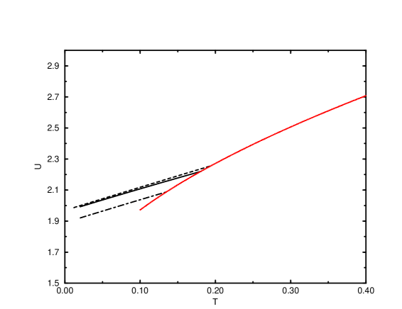
Figure 7: The internal energy versus the temperature, computed in an expansion to first order (dashed-dotted line) and second order(full line) in the cage size $A$, and in the harmonic resummation (dashed line). Also shown is the internal energy of the liquid (dotted line).

In fig. 8 we plot the specific heat versus temperature. It is basically constant and equal to 3/2. The fluctuations are numerical errors due to the extraction of the specific heat through the numerical second derivative of the free energy. A specific heat $C=3/2$ is nothing but the Dulong-Petit law (we have not included the kinetic energy of the particles, which would give an extra contribution of $3/2$). This result is very welcome: in fact if we had treated the crystal at the same level of approximation as we considered here for the glass, we would get the Einstein model for which the specific heat is also given by the Dulong-Petit law. Thus we have found that the specific heat of the glass is equal to that of the crystal, which is a good approximation of the existing data. Notice that it was not obvious at all a priori that we would be able to get such a result form our computations, since we are performing some computations purely in the liquid phase, with a liquid pair-correlation etc… The fact of finding the Dulong-Petit law is an indication that our whole scheme of computation gives reasonable results for a solid phase. At a later stage we would like to go beyond the Dulong-Petit law and get a better computation of the spectrum of soft vibration modes in order to get a Debye-like law. This is left for future work.

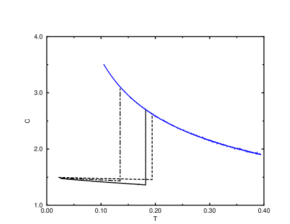
Figure 8: The specific heat of the glass versus the temperature, computed in an expansion to first order (dashed-dotted line) and second order(full line) in the cage size $A$, and in the harmonic resummation (dashed line). The dotted line is the specific heat of the liquid.

7.6 Configurational entropy

In fig. 9 we show the configurational entropy versus the free energy at various temperatures, including the zero temperature case. We have included here for simplicity only the result from the harmonic resummation procedure.

Figure 9: The configurational entropy $\Sigma(f)$ versus the free energy, computed within the harmonic resummation, at temperatures $T=0.,.05,.1$ (from left to right).

We notice that the various curves corresponding to different temperatures are not far from being just shifted one from another by adding a constant to the free energy. This indicates that the main effect of temperature amounts to an additive constant in the energies of all amorphous packings. This would be the case if the states at finite temperature could be deduced continuously from the zero temperature amorphous packings, with an extra contribution to the free energy coming from the vibrations, if the vibration spectrum is more or less state independent.

7.7 Dynamical transition

As we discussed in the introduction, at the mean field level there exists a dynamical transition at a temperature $T_{D}$ larger than the thermodynamic transition temperature $T_{K}$. This phase is characterized by the dynamic statement that a system will remain forever in the same valley, and its free energy is greater than the equilibrium one because it misses the contribution of the configurational entropy. It is thus evident that this dynamic phase is just a mean field concept, which should disappear when corrections, such as activated processes, due to the short range nature of the potential, are taken into account. However if the barriers are sufficiently high, metastable states have a very large life time and they strongly affect the dynamics. It would be thus interesting to try to compute the ‘dynamic transition temperature’ in these systems.

In the framework of the harmonic resummation one finds that the approximation breaks down at small but positive $\epsilon$ if the matrix of second derivatives has negative eigenvalues. From this point of view the appearance of negative eigenvalues signal the dynamic transition. Unfortunately in our chain approximation all the eigenvalues are positive at all temperatures and no dynamic phase transition can be seen: the free energy is always well defined for small $\epsilon$. This negative result is due to the fact that the chain approximation we use may be reasonable at low temperature but it is certainly not good at high temperatures. This problem will disappear if one uses a better method to compute the spectrum, giving reasonable results also at higher temperatures. On the other hand in the framework of the small cage expansion the perturbative method assumes that there is always a bound state. Although this should not be true at high temperature, the breakdown of this assumption cannot be seen in a perturbative approach.

It is clear that a study of the dynamical phase transition should be done using some different tools than the one we have developed here. This is not surprising: the dynamical phase transition is present at a temperature higher than the static one and the approximations which we have been using are low temperature ones.

8 Discussion and perspectives

Deducing the thermodynamic properties of the glass from those of a liquid may look crazy. Of course the main trick is that we use a molecular liquid, with a variable number $m$ of atoms per molecule, which will have a glass transition at a temperature lower than $T_{K}$ whenever $m<1$. We wish to underline again what is the basic hypothesis of our approach. We assume that there exists a thermodynamic glass transition, which is of the general type described in our ‘basic scenario’. This assumption means that there exists a path in the $m\ ,\ T$ space which connects the points $m<1\ ,\ T^{(m)}$ to the high temperature region without crossing any transition. If this is true (and this is known to happen in many models) the situation is rather simple and corresponds to what is called in the literature one step replica symmetry breaking. This situation corresponds to the case in which the deep minima of the free energy are completely uncorrelated [22, 46]. One could think of checking this hypothesis numerically by computing for small systems all the metastable states at zero temperature, and studying the distribution of their energies. Let us mention for completeness that there exist models in which the deep minima of the free energy are partially correlated (this is very probably the case of spin glasses [47, 48]). In such a case any path in the $m-T$ space which connects the point $(m,T^{(m)})$ to the high temperature region crosses a phase transition, and one would need to introduce a more complex construction in order to avoid this singularity.

The approach described in this paper opens the way to the computation of the thermodynamic properties of glasses at all temperatures using the generalization of the standard tools of liquid theory. Although it is not explicitly discussed in this paper, this approach allows also the computation of the density correlation function $g(r)$ in the glassy phase; we plan to address this point in the next future.

It is clear that the results presented here just use the simplest possible non trivial approximations. Nevertheless, within these simple approximations, we have shown that a reasonable value of the Kauzman temperature can be derived, as well as several thermodynamic properties of the glass phase: the internal energy, free energy, configurational entropy and specific heat, and the cage radius. Obviously our study so far has been restricted to equilibrium properties, and the equilibrium situation is very difficult to reach experimentally. However one can think of measuring each of the above properties in numerical simulations, where the joint use of smart algorithms and small enough system can allow to thermalize. The extension of the present methods to binary mixtures is a work that must be done in order to allow for a more precise comparison with the results of numerical simulations. Some steps have already been done in this direction [40].

This equilibrium study is to be considered as a first step before dealing with the out of equilibrium dynamics. Beside the dynamics in the low temperature phase, a very interesting and open problem is the computation of the time dependent correlation functions (and as a by-product the viscosity) in the region above $T_{K}$. However a better understanding of activated processes in this framework is a crucial prerequisite.

Within the equilibrium framework, we have implemented so far our general strategy using rather crude methods. These should be improved, which means that one must perform a more careful study of the molecular liquid. There are many directions in which one could move:

• Improve the computation of the spectrum in the harmonic approximation. This harmonic approximation should be excellent and allow to study from first principles all the low temperature anomalies which have been observed in glasses. Within this approximation one just needs to study the liquid of the centers of masses of the molecules, which interact through the effective interaction described in (41). Of course the interaction term coming from the $\mbox{Tr}\log$ term is not easy to deal with, but still this is a very well defined problem of liquid theory for which precise approximation scheme should be developed.

• Use approximations different from HNC, which may work better in the liquid phase. Obviously this will depend on the interaction potential, and a detailed study of several different types of potentials would be very interesting.

• Use numerical simulation in the liquid phase in order to get some higher order coefficients of the $A$ expansion: these are given by higher order correlation functions which could be measured in simulations.

• Introduce resummation techniques that are more efficient than the harmonic one.

Some of the previous described techniques could also be used to understand better the properties of the dynamical phase transition.

To summarize, our approach transforms the problem of the thermodynamics of the glass phase into a problem of a (complicated) liquid state. We hope that the sophisticated methods developed in liquid state theory will be brought to bear on the study of glasses.

Appendix I: HNC closure

For completeness, we give here a derivation of the HNC free energy (55) for our molecular replicated system. One could use the standard diagrammatic method [56], but here we shall follow the ’cavity’ like method of Percus [57]. We study $N$ molecules with coordinates $x_{i},i\in\{1,..,N\}$. Each $x_{i}$ stands for the coordinates of all atoms in molecule $i$: $x_{i}=\{x_{i}^{a}\},a\in\{1,...,m\}$. The energy of the system is given by

$$E=\sum_{i<j}V(x_{i},x_{j})+\sum_{i}u(x_{i})$$ (81)

where $v$ is the intermolecular potential (in our case we would have $V(x,y)=\sum_{a}v(x^{a}-y^{a})$ but we shall keep a general $V$ in this appendix), and the external potential $u(r)$ has been introduced for future use.

We shall need the following definitions. The one molecule density is

$$\rho(x)=\sum_{i}\langle\prod_{a}\delta(x_{i}^{a}-x^{a})\rangle\ ,$$ (82)

where the average $\langle.\rangle$ is with respect to the Boltzmann measure $\exp(-\beta E)$. The two molecules correlation is:

$$\rho^{(2)}(x,y)=\sum_{i\neq j}\langle\prod_{a}\delta(x_{i}^{a}-x^{a})\prod_{b}\delta(x_{i}^{b}-x^{b})\rangle\equiv\rho(x)g(x,y)\rho(y)$$ (83)

where we have also defined the pair correlation function $g(x,y)$, which goes to one at large (center of mass) distance. The connected pair correlation is:

$$h(x,y)\equiv g(x,y)-1$$ (84)

Elementary functional differentiation gives:

$${\partial\rho(x)\over\partial(-\beta u(y))}=\rho(x)\delta(x-y)+\rho(x)h(x,y)\rho(y)$$ (85)

One can also introduce the direct correlation function $c(x,y)$ through:

$${\partial(-\beta u(x))\over\partial\rho(y)}={1\over\rho(x)}\delta(x-y)-c(x,y)$$ (86)

the direct correlation is thus related to the connected pair correlation through the Ornstein-Zernike equation $c=(1+h\rho)^{-1}h$ which reads more explicitly:

$$c(x,y)=h(x,y)+\int dx_{1}h(x,x_{1})\rho(x_{1})h(x_{1},y)+\int dx_{1}dx_{2}h(x,x_{1})\rho(x_{1})h(x_{1},x_{2})h(x_{2},y)+...$$ (87)

The idea of Percus is to compute the pair correlation by considering the one point density with a molecule fixed at one point. Let us consider a problem in which we have added one extra molecule, fixed at a point $z=\{z^{1},...,z^{m}\}$. This extra molecule creates an external potential $u(x)=V(x,z)$. The one point density in the presence of this external potential, $\rho_{u}(x)$, is related to the density $\rho(x)$ and pair correlation $g(x,z)$ in the absence of an external potential through the conditional probability equation:

$$\rho_{u}(x)=\rho^{(2)}(x,z)/\rho(z)=\rho(x)g(x,z)$$ (88)

In order to try to build a successful approximation scheme, let us introduce two quantities $R_{u}(x)$ and $S_{u}(x)$ which we can calculate in presence of the external potential, or when this potential is turned off ($u=0$). If their variations are smooth enough, one can approximate their variations by the first order term:

$$R_{u}(x)\simeq R_{u=0}(x)+\int dy{\delta R(x)\over\delta S(y)}_{u=0}\left(S_{u}(y)-S_{u=0}(y)\right)$$ (89)

The standard perturbation theory would be obtained by taking $R_{u}(x)=\rho_{u}(x)$ and $S_{u}(x)=u(x)$. However the linear truncation (89) can be better behaved with some better choices of the functions $R$ and $S$. The HNC closure corresponds to taking [57]:

$$R_{u}(x)=\log\left(\rho_{u}(x)e^{\beta u(x)}\right)\ \ \ ;\ \ \ S_{u}(x)=\rho_{u}(x)\ .$$ (90)

Then we have

$${\delta R(x)\over\delta S(y)}\left({u=0}\right)=c(x,y)$$ (91)

and the linear equation (89) becomes:

$$\log g(x,z)+\beta V(x,z)=\int dyc(x,y)\rho(y)h(y,z)$$ (92)

Together with the inversion relation (87), this defines a closed set of equations for the one and two point molecular densities which are the HNC closure. It is easy to show that these equations express the stationarity of the free energy functional $\psi[\rho,g]$ defined in (55), with respect to variations of $g$.

The result for the free energy can be deduced if we assume that:

• There exists a variational principle where the free energy is a functional of $g$ and $\rho$.

• The potential $\beta V(x)$ enters in the free energy is such a way that the internal energy takes the exact form $1/2\int dydx\rho(x)\rho(y)g(x,y)V(x,y)$.

• The free energy functional at $g=1$ and $v=0$, which depends only on $\rho$ is given by the exact form

  $${\beta\over m}\int\prod_{a}d^{d}x^{a}\ \rho(x)\log{\rho(x)\over e}$$ (93)

These three conditions fix in a unique way the free energy functional and are satisfied in the previous approach. Indeed the second condition implies that the free energy $\psi$ can be written as

$$\beta\psi=\beta/2\int dydx\rho(x)\rho(y)g(x,y)V(x,y)+\chi[g,\rho]$$ (94)

where $\chi$ does not depends explicitly on $\beta$. If we differentiate the previous equation with respect to $g$ we find

$$\beta/2\rho(x)\rho(y)V(x,y)+{\delta\psi\over\delta g(x,y)}.$$ (95)

If we identify the previous equation with eq.(55) (after multiplication by $\rho(x)\rho(y)$) we find that the proposed free energy (eq. (92)) has the same derivative with respect to $g$ of the exact one. Now the only ambiguity that remains in the free energy is its value at $g=1$ and $v=0$, which is fixed from the condition (3).

Appendix II: Second order small cage expansion

Here we carry out the small cage expansion of the molecular HNC equations to second order. We start from the HNC free energy (55), we introduce the center of mass and relative coordinates, $x^{a}=X+u^{a}$ and $y^{a}=Y+u^{a}$, and we expand in the cage size $A$, using the molecular density (59) and the decomposition of the correlation function given in (61).

We shall examine successively the various pieces of $2m\beta\psi$. The form of the simplest piece is deduced trivially from the constraints (62):

$$\int dxdy\ \rho(x)\rho(y)(1-g(x,y))=\int dXdY\ (1-G(X,Y))$$ (96)

(we remind that here $x$ and $y$ stand for all the molecular coordinates and are therefore $md$-dimensional vectors, while the center of mass coordinates $X$ and $Y$ are $d$-dimensional).

We go next to the piece involving the potential:

$$\beta\sum_{a}\int dxdy\ \rho(x)\rho(y)\ v(x^{a}-y^{a})g(x,y)\ .$$ (97)

We expand the potential as:

$$\sum_{a}v(x^{a}-y^{a})=mv(X-Y)+{1\over 2}\sum_{\mu\nu}v_{\mu\nu}(X-Y)\sum_{a}(u^{a}_{\mu}-v^{a}_{\mu})(u^{a}_{\nu}-v^{a}_{\nu})+...$$ (98)

and expand the correlation according to (61). Thanks to the constraint (62), the term in $mv(X-Y)$ contributes exactly as:

$$m\int dXdY\ G(X-Y)v(X-Y)$$ (99)

to all orders in $u,v$. The term in $v_{\mu\nu}(X-Y)$ contributes a piece of order $A$ which is:

$$\int dXdY\rho(u)du\rho(v)dv\ G(X-Y)\sum_{\mu\nu}v_{\mu\nu}(X-Y)\sum_{a}(u^{a}_{\mu}-v^{a}_{\mu})(u^{a}_{\nu}-v^{a}_{\nu})$$ (100)

and a piece of order $A^{2}$ which is:

$$\int dXdY\rho(u)du\rho(v)dv\sum_{\mu\nu}v_{\mu\nu}(X-Y)\sum_{a}(u^{a}_{\mu}-v^{a}_{\mu})(u^{a}_{\nu}-v^{a}_{\nu})$$ (101)

$$\left[S_{\mu\nu}(X-Y)\left(\sum_{b}[u^{b}_{\mu}u^{b}_{\nu}+v^{b}_{\mu}v^{b}_{\nu}]-2K_{\mu\nu}\right)+T_{\mu\nu}(X-Y)\left(\sum_{b}[(u^{b}_{\mu}-v^{b}_{\mu})(u^{b}_{\nu}-v^{b}_{\nu})]-2K_{\mu\nu}\right)\right]$$

The last piece of order $A^{2}$ comes from the fourth derivative of $v$ in (98):

$$\int dXdY\rho(u)du\rho(v)dv\ G(X-Y)\sum_{\mu\nu\rho\sigma}v_{\mu\nu\rho\sigma}(X-Y)\sum_{a}(u^{a}_{\mu}-v^{a}_{\mu})(u^{a}_{\nu}-v^{a}_{\nu})(u^{a}_{\rho}-v^{a}_{\rho})(u^{a}_{\sigma}-v^{a}_{\sigma})$$ (102)

Notice that the use of (62) allow us to find the order $A^{2}$ expression without ever introducing the order $A^{2}$ term in the expansion of the pair correlation. This will also be true for the other contributions below. This strategy is crucial for keeping the computation not too big. The various pieces are now easily computed using the fact that $u$ and $v$ variables are gaussian distributed with the second moment given in (60). We get:

$$\beta\sum_{a}\int dxdy\rho(x)\rho(y)\ v(x^{a}-y^{a})g(x,y)=V\int dXG(X)\left(mv(X)+A(m-1)\sum_{\mu}v_{\mu\mu}(X)\right)$$

$$+VA^{2}(m-1)\int dX\sum_{\mu\nu}\left(2S_{\mu\nu}(X)v_{\mu\nu}(X)+4T_{\mu\nu}(X)v_{\mu\nu}(X)+{m-1\over 2m}v_{\mu\mu\nu\nu}(X)\right)$$ (103)

We now turn to the ‘$g\log g$’ term in the free energy $2m\beta\psi$. Expanding as before, we get:

$$\int dxdy\rho(x)\rho(y)g(x,y)\log g(x,y)=\int dXdYG(X-Y)\log G(X-Y)+$$ (104)

$$+\int dXdY\rho(u)du\rho(v)dv\ {1\over 2G(X-Y)}\sum_{\mu\nu\rho\sigma}$$

$$\left[S_{\mu\nu}(X-Y)\left(\sum_{b}[u^{b}_{\mu}u^{b}_{\nu}+v^{b}_{\mu}v^{b}_{\nu}]-2K_{\mu\nu}\right)+T_{\mu\nu}(X-Y)\left(\sum_{b}[(u^{b}_{\mu}-v^{b}_{\mu})(u^{b}_{\nu}-v^{b}_{\nu})]-2K_{\mu\nu}\right)\right]$$

$$\left[S_{\rho\sigma}(X-Y)\left(\sum_{b}[u^{b}_{\rho}u^{b}_{\sigma}+v^{b}_{\rho}v^{b}_{\sigma}]-2K_{\rho\sigma}\right)+T_{\rho\sigma}(X-Y)\left(\sum_{b}[(u^{b}_{\rho}-v^{b}_{\rho})(u^{b}_{\sigma}-v^{b}_{\sigma})]-2K_{\rho\sigma}\right)\right]$$

which gives after performing the gaussian $u$ and $v$ integrals:

$$V\int dX \left(G(X)\log G(X)+{4A^{2}(m-1)\over G(X)}\sum_{\mu\nu}\right.$$ (105)

$$\left.\left[{1\over 2}S_{\mu\nu}(X)S_{\mu\nu}(X)+S_{\mu\nu}(X)T_{\mu\nu}(X)+T_{\mu\nu}(X)T_{\mu\nu}(X)\right]\right)$$

We now study the last piece of $2m\beta\psi$, namely the convolution term

$$\sum_{p=3}^{\infty}{(-1)^{p}\over p}\int dx_{1}...dx_{p}\ \rho(x_{1})h(x_{1},x_{2})\rho(x_{2})h(x_{2},x_{3})...\rho(x_{p})h(x_{p},x_{1})\ .$$ (106)

Here again each $x_{j}$ is a $md$ dimensional vector including all molecular coordinate, which we decompose into the center of mass $X_{j}$ and the relative coordinates $u^{a}_{j}$. Therefore each piece $h(x_{j},x_{j+1})$ in the above product is expanded as:

$$h(x_{j},x_{j+1})=h(X_{j}-X_{j+1})$$

$$+\sum_{\mu\nu}\left[S_{\mu\nu}(X_{j}-X_{j+1})\left(\sum_{b}[u^{b}_{j,\mu}u^{b}_{j,\nu}+u^{b}_{j+1,\mu}u^{b}_{j+1,\nu}]-2K_{\mu\nu}\right)\right.$$

$$\left.+T_{\mu\nu}(X_{j}-X_{j+1})\left(\sum_{b}[(u^{b}_{j,\mu}-u^{b}_{j+1,\mu})(u^{b}_{j,\nu}-u^{b}_{j+1,\nu})]-2K_{\mu\nu}\right)\right]$$ (107)

We notice again that higher order terms do not contribute to order $A^{2}$. The second order terms generated by the expansion (107) when it is inserted into (106) are obtained by picking up the ‘$h(X_{j}-X_{j+1})$’ contribution in all but two values of $j$. In order for the result not to vanish (because of (62)), we need that this two special values of $j$ be neighbours. We thus get the following order $A^{2}$ contribution to the convolution term:

$$\sum_{p=3}^{\infty} {(-1)^{p}} \int dX_{1}...dX_{p}\ \rho(u_{1})du_{1}...\rho(u_{p})du_{p}\$$ (108)

$$\sum_{\mu\nu\rho\sigma}\left[S_{\mu\nu}(X_{1}-X_{2})\left(\sum_{b}[u^{b}_{1,\mu}u^{b}_{1,\nu}+u^{b}_{2,\mu}u^{b}_{2,\nu}]-2K_{\mu\nu}\right)+\right.$$

$$\left.T_{\mu\nu}(X_{1}-X_{2})\left(\sum_{b}[(u^{b}_{1,\mu}-u^{b}_{2,\mu})(u^{b}_{1,\nu}-u^{b}_{2,\nu})]-2K_{\mu\nu}\right)\right]$$

$$\left[S_{\rho\sigma}(X_{1}-X_{2})\left(\sum_{b}[u^{b}_{1,\rho}u^{b}_{1,\sigma}+u^{b}_{2,\rho}u^{b}_{2,\sigma}]-2K_{\rho\sigma}\right)+\right.$$

$$\left.T_{\rho\sigma}(X_{1}-X_{2})\left(\sum_{b}[(u^{b}_{1,\rho}-u^{b}_{2,\rho})(u^{b}_{1,\sigma}-u^{b}_{2,\sigma})]-2K_{\rho\sigma}\right)\right]$$

$$h(X_{3}-X_{4})...h(X_{p-1}-X_{p})h(X_{p}-X_{1})$$

After performing the gaussian $u$ and $v$ integrals, we find an expression in terms of the Fourier transformed functions $h(k)$, $S_{\mu\nu}(k)$ and $S_{\mu\nu}(k)$:

$$2VA^{2}(m-1)\sum_{p=3}^{\infty}{(-1)^{p}}\sum_{\mu\nu}\int{d^{d}k\over(2\pi)^{3}}h(k)^{p-2}\left(S_{\mu\nu}(k)+T_{\mu\nu}(k)\right)^{2}$$ (109)

involving a simple geometric series.

Grouping together all the pieces of the free energy $\psi$ which we have considered, we obtain the second order expression of the free energy used in (64-68).

References

- [1] Recent reviews can be found in: C.A. Angell, Science, 267, 1924 (1995) and P.De Benedetti, ‘Metastable liquids’, Princeton University Press (1997). An introduction to the theory is: J.Jäckle, Rep.Prog. Phys. 49 (1986) 171. Some introduction to the very recent developments in connection with the spin glass ideas is given in: G. Parisi, Proceedings of the ACS meeting, Orlando (1996), cond-mat/9701068, Lecture given at the Sitges conference, June 1996 cond-mat/9701034 and Lectures given at the Varenna summer school 1996, cond-mat/9705312.
- [2] G. Parisi Phys.Rev.Lett. 78(1997)4581
- [3] W. Kob and J.-L. Barrat, Phys.Rev.Lett. 79 (1997) 3660.
- [4] J.-L. Barrat and W. Kob, cond-mat/9806027.
- [5] S.Franz and G. Parisi, Phys.Rev.Lett. 79 (1997) 2486, and cond-mat/9711215.
- [6] B.Coluzzi and G.Parisi, cond-mat/9712261.
- [7] T.M. Nieuwenhuizen, Phys.Rev.Lett. 79 (1997) 1317.
- [8] A.W. Kauzman, Chem.Rev 43 (1948) 219.
- [9] G. Adams and J.H. Gibbs J.Chem.Phys 43 (1965) 139; J.H. Gibbs and E.A. Di Marzio, J.Chem.Phys. 28 (1958) 373.
- [10] J.-P. Bouchaud, L. Cugliandolo, J. Kurchan, M Mézard, Physica A 226, 243 (1996).
- [11] T.R. Kirkpatrick and P.G. Wolynes, Phys. Rev. A34, 1045 (1986); T.R. Kirkpatrick and D. Thirumalai, Phys. Rev. Lett. 58, 2091 (1987); T.R. Kirkpatrick and D. Thirumalai, Phys. Rev. B36, 5388 (1987); T.R. Kirkpatrick, D. Thirumalai and P.G. Wolynes, Phys. Rev. A40, 1045 (1989).
- [12] D.J. Gross and M. Mézard, Nucl. Phys. B240 (1984) 431.
- [13] See for instance G.Parisi, cond-mat/9801034 and C. Donati, S.C. Glotzer, P.H. Poole, cond-mat/9811145.
- [14] J.-P. Bouchaud and M. Mézard; J. Physique I (France) 4 (1994) 1109. E. Marinari, G. Parisi and F. Ritort; J. Phys. A27 (1994) 7615; J. Phys. A27 (1994) 7647.
- [15] P.Chandra, L.B.Ioffe and D.Sherrington, Phys. Rev. lett. 75 (1995) 713, and cond-mat/9809417. P.Chandra, M.V. Feigelman and L.B.Ioffe, Phys. Rev. lett. 76 (1996) 4805.
- [16] E. Marinari, G. Parisi and F. Ritort, cond-mat/9410089. S. Franz and J. Hertz, Phys. Rev. Lett. 74, 2114 (1995).
- [17] R. Monasson, Phys. Rev. Lett. 75 (1995) 2847.
- [18] S. Franz, G. Parisi, J. Physique I 5 (1995) 1401.
- [19] M.Mézard and G.Parisi, J. Phys. A 29 65155 (1996).
- [20] M.Mézard and G.Parisi, cond-mat/9807420.
- [21] F.H. Stillinger, Science 267 (1995) 1935, and references therein.
- [22] M .Mézard, G. Parisi and M.A. Virasoro, Spin glass theory and beyond, World Scientific (Singapore 1987).
- [23] G. Parisi, Field Theory, Disorder and Simulations, World Scientific, (Singapore 1992).
- [24] An introduction to Kepler’s conjecture and some description of the recent work by T.C.Hales which may have established the conjecture can be found on the web site: www.math.lsa.umich.edu/ hales/countdown/.
- [25] A. Crisanti and H.-J. Sommers, J. Phys. I (France) 5, 805 (1995); A. Crisanti, H. Horner and H-J Sommers, Z.Phys. B 92, 257 (1993)
- [26] J. Kurchan, G. Parisi, and M. A. Virasoro, J. Phys. I France 3, 1819 (1993).
- [27] For a careful analysis of the free energy landscape see A. Cavagna, I. Giardina and G. Parisi, J. Phys. A: Math. Gen. 1997, 30, 7021 and references therein.
- [28] M. Mézard, cond-mat/9812024, to appear in Physica A.
- [29] A. Barrat, R. Burioni, and M. Mézard, J. Phys. A 29, L81 (1996).
- [30] L. F. Cugliandolo and J.Kurchan, Phys. Rev. Lett. 71, 1 (1993).
- [31] G. Parisi, in The Oskar Klein Centenary, ed. by U. Lindström, World Scientific, (1995), Il nuovo cimento 16, 939 (1994).
- [32] H.Z.Cummins et al., Phys.Rev. E47 (1993) 4223.
- [33] See the review by W.Kob, cond-mat/9809268, and references therein.
- [34] L. C. E. Struik; Physical aging in amorphous polymers and other materials (Elsevier, Houston 1978).
- [35] J.-P. Bouchaud, L. Cugliandolo, J. Kurchan., M Mézard, in ”Spin glasses and random fields”, A.P.Young editor, Worlds Scientific 1998.
- [36] S. Franz and M. Mézard Europhys. Lett. 26 (1994) 209; Physica A 210 (1994) 48.
- [37] L. F. Cugliandolo and J.Kurchan, J. Phys. A 27 (1994) 5749.
- [38] For a review see W. Gotze, Liquid, freezing and the Glass transition, Les Houches (1989), J. P. Hansen, D. Levesque, J. Zinn-Justin editors, North Holland.
- [39] J.-P. Bouchaud; J. Phys. France 2 (1992) 1705.
- [40] B. Coluzzi, Paolo Verrocchio , M. Mézard and G.Parisi, in preparation.
- [41] T. Geszti, J.Phys. C 16(1983)5805. See also E.Leutheusser, Phys.Rev. A 29 (1984) 2765 and U.Bendtzelius, W.Götze and A. Sjölander, J. Phys. C17 (1984) 5915. More reference to the existing literature can be found in [38].
- [42] Similar order parameters are also used in the study of randomly crosslinked macromolecules (see the review by P.M. Goldbart, H.E. Castillo and A. Zippelius Adv. Phys. 45 (1996) 393), with the important difference that the molecules are distinguishable because of the cross links, and cannot get out of their traps.
- [43] G.Toulouse, in ”Heidelberg colloquium on spin glasses”, I. Morgenstern and L. van Hemmen eds., Springer Verlag 1983.
- [44] S. Caracciolo, G. Parisi, S. Patarnello and N. Sourlas, Europhys. Lett. 11, 783 (1990).
- [45] M.Cardenas, S. Franz and G. Parisi, cond-mat/99712099.
- [46] J.-P. Bouchaud and M.Mézard, J.Phys. A30 (1997) 7337.
- [47] S. Franz and H. Rieger Phys. J. Stat. Phys. 79 749 (1995).
- [48] E. Marinari, G. Parisi, F. Ricci-Tersenghi, J.J. Ruiz-Lorenzo Violation of the Fluctuation Dissipation Theorem in Finite Dimensional Spin Glasses, cond-mat /9710120.
- [49] See for instance T. Keyes, J.Phys.Chem. A 101 (1997) 2921, and references therein.
- [50] Y. Wan and R.M.Stratt, J.Chem.Phys. 100 (1994) 5123, and references therein.
- [51] B. Bernu, Y. Hiwatari and J.P. Hansen, J.Phys. C18, L371 (1985); J.N. Roux, J.L. Barrat and J.P. Hansen,J.Phys. C1 7171 (1989).
- [52] G.Daldoss, O.Pilla, G. Viliani and G. Ruocco, cond-mat/9804113.
- [53] J.P.K. Doye, M. Miller and D.J. Wales, cond-mat/9808265.
- [54] L.Angelani, G.Parisi, G.Ruocco and G.Viliani cond-mat/9803165 (1998).
- [55] E.R. Nowak, J.B. Knight, E. Ben-Naim, H.M. Jaeger and S.R. Nagel, Phys. Rev. E 57 (1998) 1971.
- [56] See for instance J.P. Hansen and I.R. Macdonald, ”Theory of simple liquids”, (Academic, London, 1986), or H.N.V. Temperley, J.S. Rowlinson and G.S. Rushbrooke, ”Physics of simple liquids”, NorthHolland (Amsterdam 1968).
- [57] J.K. Percus, in The Equilibrium Theory of Classical Fluids, ed. H.L. Frisch and J.L. Lebowitz (New York: Benjamin; 1964).