Negative Specific Heat in Astronomy, Physics and Chemistry

Abstract

Starting from Antonov’s discovery that there is no maximum to the entropy of a gravitating system of point particles at fixed energy in a spherical box if the density contrast between centre and edge exceeds 709, we review progress in the understanding of gravitational thermodynamics.

We pinpoint the error in the proof that all systems have positive specific heat and say when it can occur. We discuss the development of the thermal runaway in both the gravothermal catastrophe and its inverse.

The energy range over which microcanonical ensembles have negative heat capacity is replaced by a first order phase transition in the corresponding canonical ensembles. We conjecture that all first order phase transitions may be viewed as caused by negative heat capacities of units within them.

We find such units in the theory of ionisation, chemical dissociation and in the Van der Waals gas so these concepts are applicable outside the realm of stars, star clusters and black holes.

Institute of Astronomy, University of Cambridge, CB3 0HA

and Clare College,

Senior Fellow visiting The Queen’s University, Belfast. BT7 1NN

1 Introduction

When I first used the concept of Negative Specific Heat[1] (or more correctly Negative Heat Capacity) to explain Antonov’s remarkable Gravothermal Catastrophe[2] the Statistical Mechanics community thought I was talking nonsense. But all astronomers had known since the late 1800s that adding energy to a star or a star cluster would make it expand and cool down[3]. Astronomers enjoyed this incongruous result, but had not seen it as a real paradox in thermodynamics until Thirring[4] emphasised that there is a theorem that specific heats are positive. The ‘proof’ as given in Schrödinger’s beautiful book[5] is so simple that it is most surprising that it could ever be WRONG.

Consider a canonical ensemble in thermal equilibrium

$$<\!E\!>=\sum_{i}E_{i}\exp\left(-\beta E_{i}\right)\bigg{/}\sum_{i}\exp\left(-\beta E_{i}\right)$$

$$C_{V}={d<\!E\!>\over dT}=-k\beta^{2}\,{d<\!E\!>\over d\beta}=k\beta^{2}<(E_{i}-<\!E\!>)^{2}>$$

the final expression, which follows from an elementary evaluation of $d<\!E\!>/d\beta$ via (1), is clearly positive, Q.E.D. However, the Astronomers’ argument is hardly more complicated and involves the kinetic energy $\cal T$.

The Virial theorem for a steady state under a potential energy, $\cal V$, that scales like $r^{-n}$ reads [for external (or edge) pressure $p_{e}$ and volume $V={4\over 3}\pi r^{3}_{e}$],

$$2{\cal T}+n{\cal V}=3p_{e}V\ .$$

For gravity $n=1$ and the total energy, $E$, is the sum of kinetic and potential parts. So for an isolated gravitational system $(p_{e}=0)$

$$E=-{\cal T}<0$$

but for particles in motion ${\cal T}={3\over 2}NkT$ so

$${dE\over dT}=C_{V}=-{3\over 2}Nk\ ,$$

which is clearly negative!

Luckily Thirring[4] saw how to resolve the paradox and I like to think he did so in favour of the astronomers but let me give you the historical development without first unravelling the paradox.

Antonov[2] took $N$ particles in a spherical box of radius $r_{e}$ and released them with energy $E$. The total mass was $M=Nm$. To find the most probable state he looked for a local maximum in the Boltzmann Entropy

$$S=-k\int f\,{\rm ln}\,fd^{6}\tau$$

subject to the constraints

$$N=\int fd^{6}\tau$$

$$E=\int f{p^{2}\over 2m}\,d^{6}\tau-{1\over 2}\int\!\!\int Gm^{2}{ff^{\prime}\over|{\bf r}-{\bf r}^{\prime}|}\,d^{6}\tau d^{6}\tau^{\prime}\ .$$

The integrals are taken over 6 dimensional phase space, $f$ is the distribution function and $f^{\prime}$ stands for $f({\bf r}^{\prime},{\bf p}^{\prime})$. The density $\rho({\bf r})=\int mfd^{3}p$ and $d^{6}\tau=d^{3}rd^{3}p$, As others had done, Antonov showed that the maximising $f$ was a function of $\epsilon={1\over 2}p^{2}/m-m\psi$ where $\psi$ is the gravitational potential determined self-consistently and this leads to $\psi$ obeying the equation for the isothermal gas sphere, as tabulated by Chandrasekhar[6]. We are all used to the entropy being very sharply peaked about the most probable state so no-one prior to Antonov had bothered to check whether the stationary entropy states were in fact maxima. Antonov found there was indeed a local maximum whenever the radius, $r_{e}$, of the bounding sphere was not too large, and, as $r_{e}$ was increased, the density at the edge, $\rho_{e}$, dropped compared with that at the centre, $\rho_{c}$, due to the gravity. However, when $\rho_{e}/\rho_{c}$ dropped below $1/709$, he found the point of stationary entropy ceased to be a local maximum and became a minimax. Moreover he was able to demonstrate that there is no global maximum to $S$ at any fixed $E$ so that even when maxima exist they are only local maxima.

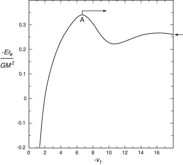
Figure 1: The dimensionless binding energy $-Er_{e}/(GM^{2})$ of an isothermal gravitating sphere of mass $M$ in a spherical container of radius $r_{e}$ plotted as a function of the density contrast, ${\rm ln}\rho_{c}/\rho_{e}=-v_{1}$, between centre and edge. Instability sets in at $A$, the maximum.

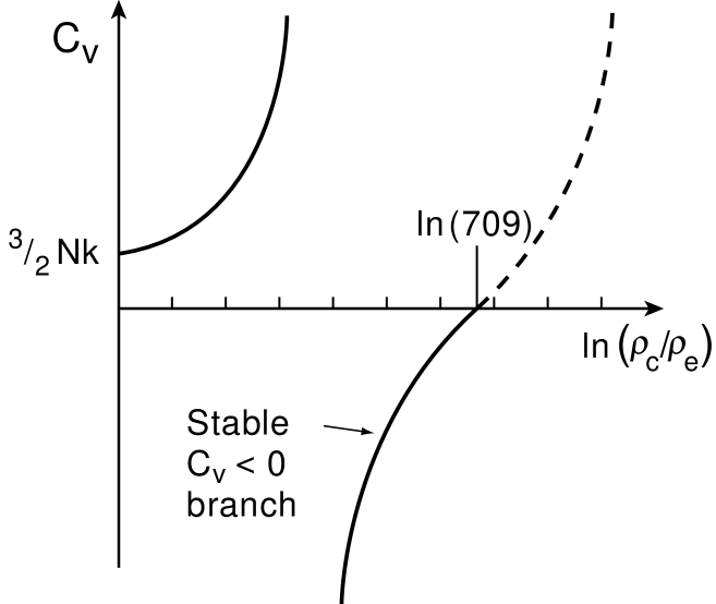
Figure 2: The specific heat $C_{V}=dE/dT$ for a self-gravitating sphere in a spherical container plotted as a function of the density contrast. Instability sets in at $A$ as $C_{V}$ reaches zero FROM BELOW!

Like many original results Antonov’s were at first hard to believe. It was particularly strange to me that the trouble occurred not when the sphere was too small, where the gravity would be large, but when the sphere was too large. Nevertheless the effect was due to gravity as it disappeared when gravity was absent. To discover what was happening I developed with Wood the thermodynamic theory of self-gravitating gas spheres[1]. In particular we calculated the energy $E$ and the heat capacity $C_{V}$ of isothermal spheres and drew the $p_{e},V$ diagram for adiabats. Figures 1, 2 & 3.

Figure 1 shows that $(-E)r_{e}/(GM^{2})$ never exceeds 0.335 for any equilibrium gas sphere, whatever the central concentration $\rho_{c}/\rho_{e}$; so, if a mass $M$ of particles is released with energy $E$ (negative) within a sphere of radius $r_{e}$ greater than $r_{A}=0.335GM^{2}/(-E)$, there is no equilibrium state for them to go to! Furthermore when $r_{e}=r_{A}$ the density contrast is Antonov’s 709.

Figure 2 plots $C_{V}=dE/dT$ as a function of the density contrast. $C_{V}$ starts at the classical value $+{3\over 2}Nk$ for a free gas but increases and becomes infinite as the density contrast $\rho_{c}/\rho_{e}$ approaches 32.2. For larger density contrasts $C_{V}$ starts negatively infinite and increases becoming zero at the Antonov point where the density contrast is 709. At this point the entropy ceases to be a maximum at constant $r_{e}$ and $E$, so stability is lost and the dashed prolongation of the sequence is unstable (see Katz[7, 8] for the proof that they remain so). However, isothermal spheres with density contrasts between 32.2 and 709 are stable at fixed $E$ and $r_{e}$ and have negative $C_{V}$.

Years of experience with positive $C_{V}$ systems are not a good preparation for this, so let me review some obvious properties of negative $C_{V}$ systems.

1. Two negative $C_{V}$ systems in thermal contact do not attain thermal equilibrium – one gets hotter and hotter by losing energy, the other gets for ever colder by gaining energy. Thus negative $C_{V}$ systems can not be divided into independent parts each with negative $C_{V}$; so negative $C_{V}$ systems are NEVER extensive.

2. A negative $C_{V}$ system can not achieve thermal equilibrium with a large heat bath. Any fluctuation that, e.g., makes it temporary energy too high will make its temporary temperature too low and the heat flow into it will drive it to ever lower temperatures and higher energies.

3. A negative $C_{V}$ system can achieve a stable equilibrium in contact with a positive $C_{V}$ system provided that their combined heat capacity is negative. To see this imagine that the negative $C_{V}$ system ‘Minus’ is initially a little hotter (higher $T$) than the positive $C_{V}$ system ‘Plus’. Then heat will flow from Minus to Plus. On losing heat Minus will get hotter (i.e., its temperature increases) but on gaining that heat Plus will also get hotter. However, because Plus has a lesser $|C_{V}|$ its temperature is more responsive to heat gain than Minus’s is to heat loss. Thus Plus will gain temperature faster than Minus and a thermal equilibrium will be attained with both Plus and Minus hotter than they were to start with. They also attain equilibrium if Minus is initially a little cooler but the reader should think that through.

   Notice that this stability is lost as soon as Plus has the same $|C_{V}|$ as Minus; i.e., when their combined heat capacity reaches zero from below.

Now we are in a position to explain Antonov’s result via a thought experiment. Imagine a gravitating isothermal gas confined by a sphere of radius just less than $r_{A}$ and adiabatically expand the sphere. Work is done by the gas so $E$ becomes yet more negative and $r_{A}$ contracts while the sphere’s radius expands making $r_{e}>r_{A}$. The inner parts of the gravitating gas are much denser and are held in primarily by gravity so the expansion is mainly taken up by the less dense gas in the outer parts. Thus the adiabatic fall in temperature of the outer parts due to their expansion will initially be greater than the temperature fall of the inner parts. Thus there will now be a temperature gradient with the outer parts cooler than the central ones. However, as we have seen, the isothermal spheres with density contrasts greater than 32.2 have negative specific heats. As heat flows down the temperature gradient the central parts contract and get hotter while the outer parts held in by the sphere behave like a normal gas so they receive the heat and get hotter too. It is now a race; do the outer parts get hotter faster on gaining the heat than the inner parts do on losing it? Clearly if the outer parts have too great a positive heat capacity they will not respond enough and the inner parts will run away to ever higher temperatures losing more and more heat to the sluggishly responding outer parts. This is Antonov’s gravothermal catastrophe. Our criterion for this to happen is that the combined heat capacities of the inner and outer parts should reach zero from below and Figure 2 shows this happens at precisely Antonov’s point. Thus isothermal gas spheres with density contrasts greater than 709 are internally unstable and will spontaneously develop temperature differences between centre and edge. Katz & Okamoto[9] recently emphasised that the effect of fluctuations will decrease the 709 limit for simulations without very large $N$.

It is of interest to consider what happens at the end of the gravothermal runaway as the centre gets hotter and hotter and denser and denser. If Antonov’s point particles are replaced by small hard spheres these will eventually get so close that they touch. Then the modified system will eventually achieve a new higher temperature equilibrium centred on this condensed core. Thus we suggested[1] that “When the system approaches the gravothermal catastrophe the system undergoes a phase transition in which a core of hard spheres in contact with one another is formed”. Aaronson & Hansen[10] later showed this was so. The more astronomically important case of a non-relativistically degenerate Fermi Gas was likewise predicted to show the same behaviour and give white dwarf configurations with total masses below the Chandrasekhar Limit[6]. For higher mass systems the Fermi Gas becomes relativistically degenerate with a pressure-density relationship that is too soft to resist gravity, so beyond the Chandrasekhar Limit the Gravothermal Catastrophe leads to Black Holes. The fact that these too have negative heat capacities was demonstrated by Beckenstein[11] and confirmed by Hawking’s[12] exact calculation. Earlier (1969) in contemplating how quasars lived and died I predicted (Lynden-Bell[13]) that giant black holes, dead quasars, lay at the centres of most large galaxies. Although Maarten Schmidt early[14] thought this was quite likely, the idea gained acceptance only gradually until twenty five years later Miyoshi et al.[15] 1995 found a definitive case in NGC4258. Now Hubble Telescope results are widely interpreted as showing giant black holes in many systems.

These are not the result of the gravothermal catastrophe of stellar dynamics (see Section 3). More energy loss via dissipative gas dynamics and radiation from quasars is needed to get such large masses into black holes by astrophysical processes.

Thirring’s resolution of the paradox[4] we posed in §1 is that two negative specific heat systems can not be in thermal equilibrium, so an equilibrium canonical ensemble of them is impossible. Thus the supposed ‘proof’ that specific heats are positive implicitly assumes the result and in reality only shows that extensive systems have positive $C_{V}$.

With Hertel[16], Thirring gave an example of a simple system with a negative $C_{V}$ for a range of energies when considered in the microcanonical ensemble. When such systems were put in thermal contact the whole showed a positive $C_{V}$ and underwent a phase-transition that corresponded to the region of negative $C_{V}$ in the microcanonical ensemble.

Some years later (1977) after Van Kampen challenged me over negative $C_{V}$, my wife and I[17] developed an easily calculable gravitational model which demonstrated these effects and predicted the temperature of the gravitational phase transition in the corresponding canonical ensemble. The model has many equal particles confined on a sphere of variable radius $r$ and is governed by the Lagrangian

$$L=\sum^{N}_{i=1}{\textstyle{1\over 2}}mr^{2}\left({\dot{\theta}}^{2}_{i}+\sin^{2}\theta{\dot{\phi}}^{2}_{i}\right)+{\textstyle{1\over 2}}M{\dot{r}}^{2}+{\textstyle{1\over 2}}GM^{2}/r,\ \ r_{0}\leq r\leq r_{e}$$

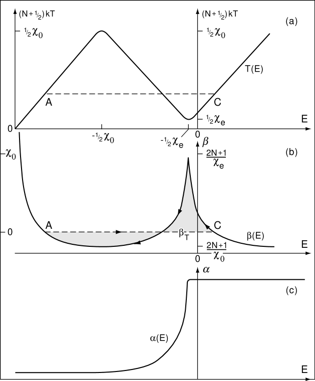
Figure 4: (a) $T$ as a function of $E$ for the variable radius slippery sphere model. $AC$ is the phase transition predicted for a canonical ensemble but replaced in practice, if $N$ is large, by lines to the maximum ($T$ increasing) or minimum ($T$ decreasing) of the $T(E)$ curve which then shows a hysteresis loop. (b) $(kT)^{-1}$ as a function of $E$. The shaded regions are of equal area for the canonical phase transition. (c) The mean radius of the sphere as a function of energy.

and $r$ is constrained to lie between some small $r_{0}$ and some large $r_{e}$. The particles on the sphere share energy as in a perfect gas. This system has $C_{V}=-(N+{\textstyle{1\over 2}})k$ whenever $a\equiv{\textstyle{1\over 4}}GM^{2}/(-E)$ lies between $r_{0}$ and $r_{e}$. However, it has positive $C_{V}$ whenever $r$ is up against one of its limits, i.e., whenever ‘$a$’ lies outside the range $(r_{0},r_{e})$, which of course happens at very low or very high energies, see Figure 4. When we considered many of these whole systems in a canonical ensemble the individual spheres were found against one stop or the other even when the mean energy was well within the microcanonical region of negative $C_{V}$. The ensemble now had $C_{V}>0$ and a macroscopic phase transition with a latent heat corresponding to the energy difference between the spheres on one stop and those on the other. Adding energy (heat) merely led to some of the systems formerly against the lower stop, $r_{0}$, migrating around the curve to the higher stop. Thus even macroscopic systems that have negative $C_{V}$ over a wide range of energies behave quite differently when thermally coupled at equilibrium. The whole assembly has a positive $C_{V}$ and a phase transition which we determined in detail, see Figure 4. This behaviour led us to ask whether all first order phase transitions could be viewed as due to negative specific heat systems of molecular size that might cause all phase transitions as discussed in the next section.

However, before leaving this one it is important to discuss what happens in practice as well as what happens ‘at equilibrium’ especially as the metastable superheated or supercooled regions in our model can be large. These metastable regions have the sphere against one stop or the other. Even in the canonical ensemble it takes a gigantic fluctuation to take such a metastable system over the hump. It has to gain a thermal energy comparable to the mean energy of each whole system, i.e., it needs a fluctuation $\sqrt{N}$ times the typical one. As emphasised by Parentani, Katz & Okamoto[18] for the black hole case, such fluctuations will occur almost never – i.e., once in $\exp(-N)$ independent trials. Thus to get the thermodynamic phase transition $N$ can not be large and even for $N=10$ one must wait for $\sim e^{10}$ complexions of the system. Thus these metastable regions of our large systems will be exceedingly stable and no phase transition of the canonical ensemble will be observed until the system nears the top of Figure 4a. However, once on the unstable branch the system will evolve along the downslope on the timescale of thermal diffusion and will then become so much cooler than the ensemble that on a similar timescale it climbs the other branch to regain the ‘tops’ temperature of $(N+{\textstyle{1\over 2}})kT\sim{\textstyle{1\over 2}}\chi_{0}$. If the ensemble is cooled, likewise the transition will not be observed until the temperature reaches the much lower temperature of $(N+{\textstyle{1\over 2}})kT\sim{\textstyle{1\over 2}}\chi_{e}$ when the transition will again go violently. Thus there will in practice be an enormous hysteresis compared to which ‘boiling with bumping’ will look quite petty.

Kiessling[19] has emphasised that statistical mechanics done properly gives transitions like $AC$ rather than ones associated with the ends of the metastable regions but for transitions in these macroscopic systems the path $AC$ would not be encountered in practice nor normally in simulations unless the numbers of particles involved are small. However, the metastable regions in microscopic systems can be surmounted by fluctuations with smaller energy changes so ice melts at the temperature at which water freezes rather than at a significantly higher one.

2 A Different View of the Cause of Phase Transitions

In the last section we saw how a region of $C_{V}<0$ in individual systems gave rise to a phase transition when many such systems were placed in thermal contact.

In reference 13 we asked whether all phase transitions (or at least all first order ones) can be viewed as caused by negative specific heat elements at a molecular level. Can one look at systems that undergo changes of state and identify such negative-heat-capacity elements? We shall demonstrate their existence for simple models of chemical dissociation or ionisation equilibrium and in systems like the Van der Waals gas.

We consider two types of particles, $A$ and $B$ which are in the ground state tied together in pairs $AB$. We take the forces between them to saturate when such a pair exists and shall model the interaction potential to be a $\delta$ function so a single bound state exists with binding energy $\chi$. Let $n_{AB}$ be the number density of pairs in some initial ground state. We shall model this system by a microcanonical ensemble of boxes each of volume $L^{3}=n^{-1}_{AB}$ and each containing one particle of type $A$ and one of type $B$. We shall show that each of these microsystems shows a negative specific heat when the energy of each box is just greater than the dissociation energy. Taking that as our zero point for energy we find the number of energy levels $<E$ for a system of two independent free particles is

$$\tau_{f}(E)\propto\left\{{E^{3}L^{3}\atop 0}\ ,\ {E\geq 0\atop E<0}\right.\ ,$$

while for a bound pair the number of energy levels is $\tau_{b}(E)\propto\left[(E+\chi)L^{2}\right]^{3/2}$.

The total number of energy levels $<E$ is thus $\tau(E)=\tau_{f}+\tau_{b}$. Gibbs gives both $S_{1}=k\,{\rm ln}\,\left(d\tau/dE\right)$ and $S_{2}=k\,{\rm ln}\,(\tau)$ as possible expressions for the entropy for small systems. We earlier[17] showed $S_{1}$ gave negative specific heat just above the dissociation point so here we consider $S_{2}$. Evidently

$$kT=k{dE\over dS_{2}}={\tau\over\tau^{\prime}}={(E+\chi)^{3/2}+AE^{3}\over{3\over 2}\left[(E+\chi)^{1/2}+2AE^{2}\right]}\ ,$$

where $A\propto L^{3/2}$. It is not hard to show that

$${k\over C_{V}}={dkT\over dE}=\left({\tau\over\tau^{\prime}}\right)^{\prime}$$

is negative for some (large enough) values of $L$ for energies greater than zero and on up to about $0.8\chi$ for some $L$. Thus if the system is in a large enough box, i.e., rare enough, too many dissociate as the energy is increased so the mean kinetic energy per free particle decreases because of the energy soaked up by the dissociation. In this sense negative $C_{V}$ elements are associated with chemical dissociation reactions. Much the same arguments hold for ionisation reactions at higher temperatures.

Perhaps of greater interest is the demonstration of similar phenomena in the Van der Waals gas and the following demonstration is due to R.M. Lynden-Bell my wife. We are all familiar with the dip and hump in the isotherms of the Van der Waals gas and how Maxwell’s construction replaces them with the constant pressure phase-transition that occurs in practice. This is what will happen in an extensive system with very many identical subsystems. However, at or close to the molecular level the extensivity breaks down because such tiny systems can not be readily divided into two equivalent pieces. The Van der Waals equation includes such effects in its molecular volume term $b$ and its mean molecular attraction term which reduces the effective pressure by $a\rho^{2}$. We shall assume that at a molecular level the tiny indivisible elements of Van der Waals gas actually obey Van der Waals’s equation and it is only a cooperative effect of many of them in a canonical ensemble that makes the ensemble obey the Maxwell construction and give the phase transition. We saw that this is precisely what happened when we took our gravitating systems in Section 1 and put many of them into a canonical ensemble at equilibrium. What we now show is that an element that obeys the full curve of the Van der Waals equation inevitably has a negative $C_{p}$. The hump in the Van der Waals isotherms at temperatures below the critical one gives two stable states $AB$ which share the same temperature and pressure (the third is unstable). Thus

$$0=\Delta p=\int^{B}_{A}\left({\partial p\over\partial V}\right)_{T}dV\ .$$

For this to happen $(\partial p/\partial V)_{T}$ can not have the same sign everywhere so we need an unusual region with it positive.

Now

$$C_{p}^{-1}=\left({\partial({\rm ln}T)\over\partial S}\right)_{p}$$

so normally, with $C_{p}$ positive, ${\rm ln}T$ will increase with $S$ at constant $p$. However, the states $A$ and $B$ share a common isotherm and are at the same pressure so

$$0=\Delta({\rm ln}T)=\int^{B}_{A}\left({\partial{\rm ln}T\over\partial S}\right)_{P}dS=\int^{B}_{A}{1\over C_{p}}dS\ ,$$

so $C^{-1}_{p}=\left(\partial{\rm ln}T/\partial S\right)_{p}$ must reverse sign and the graph of ${\rm ln}T$ against $S$ can not be monotonic. We have, therefore, demonstrated that for any system which has a hump in its isotherm like that in the Van der Waals gas there is a region of negative $C_{p}$. This is our prime result!

One learns at school that for perfect gases $C_{p}-C_{V}=R$ so one might expect that systems with $C_{p}$ negative would also have $C_{V}$ negative. This is not so,

$$\halign{\hbox to\displaywidth{$\hfil\displaystyle#\hfil$}\cr 0.0pt{\hfil$\displaystyle C_{p}-C_{V}=T\left({\partial S\over\partial T}\right)_{p}-T\left({\partial S\over\partial T}\right)_{V}=T\left({\partial S\over\partial V}\right)_{T}\left({\partial V\over\partial T}\right)_{p}=\hfill\cr 0.0pt{\hfil$\displaystyle\hfill{}=T\left({\partial p\over\partial T}\right)_{V}\left({\partial V\over\partial T}\right)_{p}=-\left({\partial p\over\partial V}\right)_{T}T\left({\partial V\over\partial T}\right)_{p}^{2}\ .\crcr}}}$$

Thus $C_{p}$ is only greater than $C_{V}$ at positive $T$ when, as is usually the case, $\left({\partial p\over\partial V}\right)_{T}$ is negative. But when the pressure along an isotherm increases with $V$, as in a phase transition region, $C_{p}$ is actually less than $C_{V}$. It is, therefore, a moot point whether $C_{V}$ has to be negative. Here Van der Waals’s gas is of great interest as an example because for it gives $C_{V}={3\over 2}Nk$ which is positive everywhere! Thus the hump and trough in the isotherm is associated with negative $C_{p}$ but not with negative $C_{V}$.

3 Aftermath of the Catastrophe

We earlier left our gas just undergoing the gravothermal catastrophe with the central part contracting and getting hotter while the outer part could not raise its temperature fast enough to keep up. Since the centre is now denser the Antonov point at which the density reaches $\rho_{c}/709$ is now inside the system rather than at its edge. Thus this point moves inwards through the mass. In astronomy we are primarily interested in applying this theory to a ‘gas’ in which each molecule is replaced by a star so that we deal with a star cluster or the nucleus of a galaxy. In such systems the timescale for exchanging the ‘heat’ of random stellar motion is shortest at the centre and can become very long in the outer parts. As the Antonov point moves in, the timescale of heat flow becomes shorter and the regions beyond the Antonov point are too sluggish to respond other than adiabatically. The gravothermal catastrophe occurs again and again nay continually, with ever higher densities and temperatures at ever smaller scales[20, 21, 22] and the precise form of the initial conditions is rapidly forgotten. Since the same process is occurring at ever smaller scales we expect a similarity solution with the density of the form

$$\rho(r,t)=\rho_{c}(t)\rho_{\star}(r_{\star})$$

where $r_{\star}=r/r_{c}(t)$ and $r_{c}(t)$ the core radius will be some fixed fraction of the Antonov radius $r_{A}$ where the density is $\rho_{c}/709$. Since the halo is so sluggish that it is left behind in the every quickening evolution of the centre we can put $\partial\rho/\partial t=0$ at large $r$. Hence $\dot{\rho}_{c}\rho_{\star}-{\dot{r}_{c}\over r_{c}}r_{\star}\rho_{c}\rho^{\prime}_{\star}=0$ and so we may separate the $t$ and $r_{\star}$ dependences to get

$${r_{\star}\rho^{\prime}_{\star}\over\rho_{\star}}={r_{c}\dot{\rho}_{c}\over\dot{r}_{c}\rho_{c}}=-\alpha\ .$$

Since the $\star$ variables are independent of the $t$ variables $\alpha$ must be a constant. Thus $\rho_{\star}=Ar_{\star}^{-\alpha}$ at large $r_{\star}$ and $\rho_{c}\propto r^{-\alpha}_{c}$ for all $t$.

Now the evolution of the system is due to the heat transport whose rate is determined by ${\dot{\rho}_{c}\over\rho_{c}}\propto{1\over T_{r}}$ where $T_{r}$ is the relaxation time within the Antonov radius; for it the standard formula is $T^{-1}_{r}\propto{\rho_{c}\over v^{3}_{c}}(8\pi G^{2}m\,{\rm ln}\,N)$ where $v^{2}_{c}$ is the velocity dispersion of the stars. In our self-similar collapse

$$v^{2}_{c}\propto G{4\over 3}\pi\rho_{c}r^{3}_{c}/r_{c}\propto G\rho_{c}r^{2}_{c}\propto G\rho^{1-2/\alpha}_{c}\ .$$

Hence

$${\dot{\rho}_{c}\over\rho_{c}}\propto\rho_{c}^{{3\over\alpha}-{1\over 2}}\ \ .$$

On integration we find[21, 23]

$$\rho_{c}\propto|t_{0}-t|^{-2\alpha/(6-\alpha)}\ \ \ {\rm so}\ \ \ r_{c}\propto|t_{0}-t|^{2/(6-\alpha)}\ \ .$$

Thus the core radius becomes zero and the central density formally $\rightarrow\infty$ at $t_{0}$. The core mass is

$$M_{c}\propto\rho_{c}r^{3}_{c}\propto|t_{0}-t|^{2(3-\alpha)/(6-\alpha)}$$

and the core velocity dispersion behaves as

$$v_{c}^{2}\propto GM_{c}/r_{c}\propto|t_{0}-t|^{(4-2\alpha)/(6-\alpha)}\ .$$

We must still determine $\alpha$.

Now at large distances $\rho_{\star}\propto r_{\star}^{-\alpha}$ and the asymptotic form of the constant temperature (isothermal) sphere is $\rho\propto r^{-2}$ so for an outward temperature decrease $\alpha>2$. However, if $\rho\propto r^{-2.5}$ there is an infinite binding energy near the centre and to create this in finite time would need an impossibly large heat flux. Thus from these general arguments $2<\alpha<2.5$. Detailed calculations give $\alpha$ as an eigenvalue and for stellar dynamics all investigators get $\alpha=2.22\pm.01$ which gives the rather weak dependence $v_{c}\propto|t_{0}-t|^{-(\alpha-2)/(6-\alpha)}$. From these one finds $M_{c}\propto v_{c}^{-2(3-\alpha)/(\alpha-2)}$ where the exponent is 7.1 for $\alpha=2.22$. If in core collapse $v_{c}$ increased from 300 km/s to 300,000 km/s corresponding to a black hole then $M_{c}$ would decrease by a factor $2\times 10^{21}$ leaving much less than one star so these conditions are not attained. In fact if $M_{c}$ decreased by $10^{7.1}$ then $v_{c}$ would increase by a factor 10 only. However, in fact a new phenomenon sets in a high star densities that produces a delightful new twist in the evolution. Henon[24] in his most percipient early work suggested that the formation of binary stars would occur at very high densities and that this would produce a new energy source. Heggie[25] did the seminal work on the binary creation rate and Betteweiser & Sugimoto[26] put this into their code for core collapse. As Sugimoto had surmised[27], binary formation sets in quite suddenly during core collapse and releases energy near the centre. Since the core is of negative heat capacity it immediately expands and becomes of lower temperature than its surroundings. The stage is now set for the inverse gravothermal catastrophe. As heat is conducted into the core it grows and gets colder. The process goes on until eventually the core grows so large that it contacts the cooler outer parts of the halo. Then the whole core becomes isothermal and eventually feels the heat loss to the outside so the gravothermal collapse stars again. A number of these giant thermal pulses occur in simulations of post-collapse core evolution so it is hard to tell whether the self-similar evolution[23] predicted on the basis of a singular core from which a flux of energy emerges due to continued energy emission from binaries gives even a roughly correct average evolution.

Padmanabhan[28] has given a longer more quantitative review of gravitational thermodynamics which discussed many of the phenomena considered here.

Meylan & Heggie[29] have an up to date review of the more astronomical aspects.

Miller & Youngkins[30, 31] have given the mean field theory for a simple system of spheres and have conducted numerical simulations to verify the existence of gravitational phase transitions.

Both Miller & collaborators[32] and Tsuchiya[33] have conducted very long term integrations to investigate the approach to equilibrium of a one-dimensional system of mass sheets. For these relaxation is particularly slow as the interactions when they cross are rather smooth.

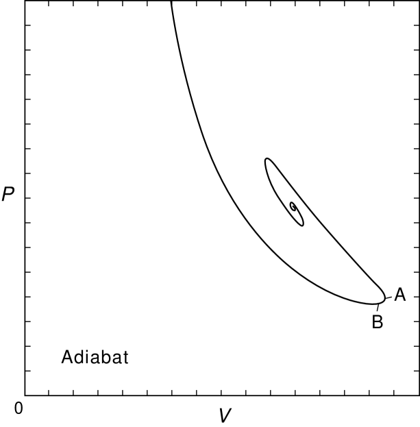
Figure 3: The adiabat plots the surface pressure of the sphere against its volume $V={4\over 3}\pi r^{3}_{e}$ at constant entropy, instability sets in at $A$ for an isolated system but at $B$ if the system is held at constant pressure.

References

- [1] Lynden-Bell, D. & Wood, R. 1968, Mon. Not. R. Astr. Soc. 138, 495.
- [2] Antonov, V.A. 1962, Vest. Leningrad Univ. 7, 135; Translation 1995, IAU Symposium 113, 525.
- [3] Eddington, A.S. 1926, The Internal Constitution of the Stars, Cambridge; see also 1916, Mon. Not. R. Astr. Soc. 76, 525.
- [4] Thirring, W. 1970, Z. Phys. 235, 339; see also Essays in Physics 4, 125.
- [5] Schrödinger, E. 1952, Statistical Thermodynamics, Cambridge.
- [6] Chandrasekhar, S. 1939, An Introduction to the Study of Stellar Structure, Dover.
- [7] Katz, J. 1978, Mon. Not. R. Astr. Soc. 183, 765.
- [8] Katz, J. 1979, Mon. Not. R. Astr. Soc. 189, 817.
- [9] Katz, J. & Okamoto, I. 1999.
- [10] Aaronson, E.B. & Hansen, C.J. 1972, ApJ 177, 145.
- [11] Beckenstein, J.D. 1974, Phys. Rev. D. 9, 3292.
- [12] Hawking, S. 1974, Nature 248, 30.
- [13] Lynden-Bell, D. 1969, Galactic Nuclei as Collapsed Old Quasars, Nature 223, 690.
- [14] Schmidt, M. 1972, Conference at the Inauguration of the South African Astronomical Observatory, Cape Town, unpublished.
- [15] Miyoshi, M., Moran, J., Hernstein, J., Greenhill, L., Nakai, N., Diamond, P. & Inoue, M. 1995, Nature 373, 127.
- [16] Hertel, P. & Thirring, W. 1971, Ann. Phys. 63, 520; see also Comm. Math. Phys. 24, 22 and 28, 159.
- [17] Lynden-Bell, D. & Lynden-Bell, R.M. 1977, Mon. Not. R. Astr. Soc. 181, 405.
- [18] Parentani, R., Katz, J. & Okamoto, I. 1995, Class. Quantum Gravity 12, 1663.
- [19] Kiessling, J. 1989, Stat. Phys. 55, 203.
- [20] Hachisu, I., Nakada, Y., Nomoto, K. & Sugimoto, D. 1978, Prog. Theor. Phys. 60, 393.
- [21] Lynden-Bell, D. & Eggleton, P.P. 1980, Mon. Not. R. Astr. Soc. 191, 483.
- [22] Cohn, H. 1980, ApJ 242, 765.
- [23] Inagaki, S. & Lynden-Bell, D. 1983, Mon. Not. R. Astr. Soc. 205, 913.
- [24] Henon, M. 1961, Annales d’Astrophysique 24, 369.
- [25] Heggie, D.C. 1975, Mon. Not. R. Astr. Soc. 173, 729.
- [26] Betteweiser, E. & Sugimoto, D. 1984, Mon. Not. R. Astr. Soc. 208, 493.
- [27] Sugimoto, D. & Betteweiser, E. 1983, Mon. Not. R. Astr. Soc. 204, 191.
- [28] Padmanabhan, T. 1990, Physics Reports 188, No.5, 285.
- [29] Meylan, G. & Heggie, D.C. 1997, Astron. Astrophys. Rev. 8, 1.
- [30] Miller, B.N. & Youngkins, P. 1997, Chaos 7, 187.
- [31] Youngkins, P. & Miller, B.N. 1997, Phys. Rev. E 56, R4963.
- [32] See, e.g., Yawn, K.R. & Miller, B.N. Phys. Rev. E 56, 2429.
- [33] Tsuchiya, T., Gondu, N. & Konishi, T. 1996, Phys. Rev. E 53, 2210.