Self-Organized States in Cellular Automata: Exact Solution

Abstract

The spatial structure, fluctuations as well as all state probabilities of self-organized (steady) states of cellular automata can be found (almost) exactly and explicitly from their Markovian dynamics. The method is shown on an example of a natural sand pile model with a gradient threshold.

Complicated dynamics of various discrete systems may naturally be modeled by CA having rather simple iteration rules. In particular, CA models are useful to study traffic jams [3], granular material dynamics [4], and self-organization [5, 6]. The transport properties of systems the, especially in the Self-Organized (SO) critical regime were extensively studied (cf., [6, 7, 8, 9, 10]). However, for many applications, one needs to know an entire structure of the SO states. These may include: (i) the temperature profiles for the convection dominated thermoconduction and turbulent convection [11] (as in the convective zone of the sun and stars), (ii) stability and average profiles of granular materials (e.g., the sand pile profiles) and granular flows [4, 5], (iii) equilibrium and steady state profiles of plasma pressure and temperature in fusion devices [10, 12], etc. Despite its importance, the problem of spatial structure and characteristics of the SO steady states has received minor attention [9, 13, 14, 15]. In this Letter, we propose a method which is equally applicable to any CA provided its rules are rather simple. We illustrate it on the simplest and popular example of an one-dimensional sand pile with a gradient stability criterion. Note that this model is the closest to a natural pile of sand created by random sprinkling of sand and with a known repose angle. We focus ourselves on calculating of an average slope (the calculation is more transparent) though calculating other characteristics is trivial.

An interesting result obtained is that the SO profiles of a local slope are non-trivial even for this simplest case. They are typically flat (e.g., linear) throughout the pile while a narrow region (similar to the boundary layer) with rapidly increasing gradient always occur near the top of the pile. This picture is very similar to that experimentally measured in a strongly turbulent convection of a passive scalar (temperature) with a mean gradient [11]. The region of the super-critical (unstable) gradient may form near the bottom of the pile when the noise is strong enough to maintain almost continuous sand flow (overlapped avalanches). This is in excellent agreement with direct numerical simulations [12].

Among many sand pile models, the Abelian model is the only one that was proved to be analytically exactly solvable [14, 16]. It is, however, rather unnatural since its stability criterion is given in terms of a site height, not slope of the pile (which depends on neighboring sites, too). Another tacit assumption is one of weak noise: no sand is added to the pile unless at least one unstable site presents (i.e., until the very last avalanche is gone). Note that “waves of toppling” [15], which are the main point of the whole analysis, are well defined in the weak noise limit, only. We show that both these restrictions may be relaxed: (i) a site stability criterion may depend on site’s neighbors and (ii) sand may be added at every time step thus affecting an avalanche dynamics. We also show that in the weak noise limit, all state probabilities can be calculated exactly in a closed form, while for the strong noise, they can be found almost exactly, i.e., with any a priori given accuracy.

For a general $N$-dimensional sand pile automaton, the procedure is following. (1) Reformulate the model in the representation where the stability is local and defined by the state of a site, alone. This can be done at expense of introducing a nonlocality to the toppling and noise rules (i.e., they may depend on states of adjacent sites too). (2) Consider the dynamics of a single site. Since toppling rules have no intrinsic memory, however, it is Markovian. Construct an $N$-dimensional Markov hyper-lattice (an analog of a Markov chain in one dimension) with the transition probabilities defined by the CA rules. All the transition probabilities which depend on states of other sites are, for now, free parameters. Introducing a generating function, one can then solve the problem for a single site. (3) Noting that all sites are identical, we relate the Markov transition probabilities for different sites. Boundary conditions then uniquely define their values and, thus, the SO state of the pile. Note that a mean-field type closure is needed at step (3), only.

Model — The model we consider consists of $L+1$ spatial sites, numbered from $x=0$ to $x=L$. To each site $x$ is assigned a variable $h(x)$, the height of the site. CA rules are applied to the pile at each time-step. Sand grains are added randomly to sites with probabilities $p_{sand}(x)$ increasing the height by one. When the site $x$ is unstable, i.e., if the local slope [difference of heights of two neighboring sites $h(x)-h(x+1)$] exceeds some critical value $\Delta h_{crit}(x)$, ${N_{f}}$ sand grains topple onto the neighboring site $x+1$ (local, limited model [6]). Note that ${N_{f}}>1$ corresponds to the physical situation where friction between sand grains at rest is greater than friction of those in motion. Sand is expelled from the pile through the right end $x=L$.

For the stability condition to be local, we represent the sand pile in “gradient space”. We assign to any site the local difference of heights of the nearest neighbors $\Delta h(x)=h(x)-h(x+1)$. Then the noise and toppling rules become, respectively:

noise $${\left\{\begin{array}[]{ll}&\Delta h(x-1)\to\Delta h(x-1)-1,\\ &\Delta h(x)\to\Delta h(x)+1;\end{array}\right.}$$ (4)

toppling $${\left\{\begin{array}[]{ll}&\Delta h(x-1)\to\Delta h(x-1)+{N_{f}},\\ &\Delta h(x)\to\Delta h(x)-2{N_{f}},\\ &\Delta h(x+1)\to\Delta h(x+1)+{N_{f}}.\end{array}\right.}$$ (8)

The left end ($x=0$) is now an open boundary (top of the pile): $\Delta h(0)\to\Delta h(0)-2{N_{f}}$, $\Delta h(1)\to\Delta h(1)+{N_{f}}$; the right end ($x=L$) is a closed boundary (bottom of the pile): $\Delta h(L-1)\to\Delta h(L-1)+{N_{f}}$, $\Delta h(L)\to\Delta h(L)-{N_{f}}$. Note that “particles” in the gradient space are not sand grains! They may enter or leave the system through the left boundary, only. Noise creates a “particle” at ${x=0}$ with the probability ${p_{sand}(0)}$, as follows from Eq. (4) for ${x=0}$. A toppling at ${x=0}$ results in a sudden loss of $N_{f}$ “particles”.

Zero-dimensional pile — Now, we may consider one site $x$, alone. It is described by a collection of states representing all possible values of local gradient. Negative states are not allowed. These states are labeled by an integer variable $k\equiv\Delta h(x)$, and the critical slope is ${Z_{c}}\equiv\Delta h_{crit}(x)$. The states $k<{Z_{c}}$ are stable, those $k>{Z_{c}}$ are unstable, and the state $k={Z_{c}}$ is marginally stable. We introduce the probabilities $p_{k}$ for a site to occupy a state $k$, i.e., to have the slope $\Delta h=k$. Due to noise and overturning events, the state of a site will evolve in time. The rules given by Eqs. (Self-Organized States in Cellular Automata: Exact Solution) are independent of previous history of a system. Therefore, they define the evolution of the slope of a site to be a Markov process. The states arranged in increasing order of $k$ form a Markov chain. Adding and toppling rules specify transition probabilities from one state to another on this chain.

1. Adding sand [Eq. (4)] results in jumps by 1 right or left (i.e., a increase or decrease gradient). The transition probabilities of the process are $\alpha$ and $\beta$, respectively, and equal: $\alpha=p_{sand}(x+1)\bigl{[}1-p_{sand}(x)\bigr{]},~{}\beta=p_{sand}(x)\bigl{[}1-p_{sand}(x+1)\bigr{]}$. Note here that adding of a sand grain in real space results in increase or decrease of a state (i.e., local slope) in gradient space.

2. Toppling of a site [Eq. (8)] results in a jump by $2{N_{f}}$ states left (i.e., a decrease in gradient). The probability of that process is ${\bf 1.~{}}$, i.e., an unstable state topple on the next time-step with the probability unity.

We introduce two “nonlocal” transition probabilities. (1) Toppling of one of two neighboring sites results in a jump by ${N_{f}}$ states right (i.e., an increase in gradient). The probability of this process is written as $\epsilon^{*}$. (2) Toppling of both two neighbors results in a jump by $2{N_{f}}$ states right. The transition probability is written as $\delta^{*}$. Both $\epsilon^{*}$ and $\delta^{*}$ are simply constants here which are to be specified in the one-dimensional model via a mean-field-type closure. Generally speaking, $\alpha,~{}\beta,~{}\epsilon^{*}$, and $\delta^{*}$ will depend on $x$ and $k$. We later consider the case where all are independent of $x$ and $k$ (homogeneous pile with no local slope dependence).

In Fig. 1, the Markov chain with all possible transitions for stable ($\bullet$) and unstable ($\circ$) states with corresponding transition probabilities is shown. Noise results in one-step random walk of a particle on this chain. Toppling of sites results in jumps by ${N_{f}}$ and $2{N_{f}}$ states. Since the noise process is statistically independent of toppling, these processes may combine with each other resulting in jumps by ${N_{f}}-1,{N_{f}}+1,2{N_{f}}-1$, and $2{N_{f}}+1$ jumps, with the probabilities respectively proportional to $\epsilon^{*}\beta,~{}\epsilon^{*}\alpha,~{}\delta^{*}\beta$, and $\delta^{*}\alpha$. All other transition coefficients are similarly defined.

We thus have reduced the problem of a sand pile to the problem of a random walk of a particle on a chain of states where the transition probabilities are exactly defined. For a general type of a Markov process the general kinetic (or master) equation is

$$\dot{p}_{n}(t)=\sum_{k=0}^{\infty}\left\{\gamma_{nk}p_{k}(t)-\gamma_{kn}p_{n}(t)\right\},$$ (9)

where $\gamma_{kn}$ are the transition probability coefficients from state $n$ to state $k$. Note that the term $\gamma_{nk}p_{k}$ describes transitions into the state $n$ from state $k$, while $\gamma_{kn}p_{n}$ corresponds to transition out of $n$ into other states $k$. This equation defines the probabilities $p_{n}$ for the system to be in state $n$. The general kinetic equation for one site can easily be written using Fig. 1. Because of space limitations, we do not write it explicitly.

We introduce a generating function for the probability distribution $p_{k}$:

$$F(\zeta,t)=\sum_{k=0}^{\infty}\zeta^{k}p_{k}(t),$$ (10)

where $\zeta$ can take values $|\zeta|\leq 1$ for a series to converge. The probability distribution can be recovered from the generating function as

$$p_{k}(t)=(1/k!)\left.d^{k}F(\zeta,t)/d\zeta^{k}\right|_{\zeta=0}.$$ (11)

Some properties of the generating function are ${F(1,t)=1},~{}{\left.F_{\zeta}^{\prime}\right|_{\zeta=1}=\left<n(t)\right>},\dots$, where ‘prime’ means derivative. Here the first is the normalization condition: ${\sum p_{j}=1}$, and second relates $F(\zeta,t)$ to the first moment (e.g., expectation value) of the probability distribution. Higher moments (i.e., standard deviation, etc.) are obtained from higher derivatives of $F(\zeta,t)$. Multiplying each of Eqs. (9) for $\dot{p}_{k}$ respectively by $\zeta^{k}$ and taking sum over all $0\leq k<\infty$, we straightforwardly obtain an equation for a generating function $F=\Phi+\Psi$. Since we are interesting only in a steady state, we set $\dot{F}=0$. Then it reads

$$F(\zeta)\{\bullet\}+\Psi(\zeta)\left(\zeta^{-2N_{f}}-1\right)\!\left[\alpha^{-1}+\{\bullet\}\right]=p_{0}\!\left(\zeta^{-1}-1\right),$$ (12)

where $\alpha=\beta,\epsilon=\epsilon^{*}/\alpha,\delta=\delta^{*}/\alpha$ and $\{\bullet\}=(\zeta+\zeta^{-1}-2)(1+\epsilon\alpha\zeta^{N_{f}}+\delta\alpha\zeta^{{2N_{f}}})+\epsilon(\zeta^{N_{f}}-1)+\delta(\zeta^{{2N_{f}}}-1).$ Here $\Phi(\zeta)=\sum_{k=0}^{Z_{c}}\zeta^{k}p_{k}$, $\Psi(\zeta)=\sum_{k={Z_{c}}+1}^{\infty}\zeta^{k}p_{k}$ are the partial generating functions of stable and unstable states, respectively.

To find $\Psi$, one may use a simple trick [using Eq. (12)]:

$$\left.\left(\frac{\partial^{Z_{c}+1+j}}{\partial\zeta^{Z_{c}+1+j}}\ \Phi(\zeta)\right)\right|_{\zeta=0}\equiv 0,\qquad j\geq 1.$$ (14)

In general, this system is an infinite set of related equations. It relates all $p_{Z_{c}+1+j}$ to $p_{0}$. Together with ${F(1)=1}$, it provides an exact solution, $F(\zeta)$, of Eq. (12). For an Abelian sand pile, the transition probabilities of simultaneous toppling and noise [e.g., toppling to higher states, ${\bf 1.}\delta^{*}\alpha$ (see Fig. 1)] vanish identically by definition. (Note, this is the limit when noise is too weak to affect avalanche dynamics.) Thus, the highest achievable state is $Z_{c}+2N_{f}$. The Markov chain is finite, and Eqs. (14) reduce (schematically) to the system with triangular matrix (with $a_{ij}$ and $b_{k}$ being constants)

$$\pmatrix{a_{1,1}\!\!\!\!&a_{1,2}&\!\!\dots\!\!&a_{1,2N_{\!f}}\cr 0\!\!\!\!&a_{2,2}&\!\!\dots\!\!&a_{2,2N_{\!f}}\cr\vdots\!\!\!\!&\vdots&\!\!\ddots\!\!&\vdots\cr 0\!\!\!\!&0&\!\!\dots\!\!&a_{2N_{\!f},2N_{\!f}}}\pmatrix{p_{Z_{c}+1}\cr p_{Z_{c}+2}\cr\vdots\cr p_{Z_{c}+2N_{\!f}}}\!=\!\pmatrix{b_{1}\cr b_{2}\cr\vdots\cr b_{2N_{\!f}}}\!p_{0}$$ (15)

which can be solved exactly and explicitly. In the opposite case, when noise is not weak, one may, however, truncate the system of Eqs. (14) to a finite hierarchy simply by noticing that the probabilities $p_{Z_{c}+2N_{f}+j}$, $j\geq 1$ are very low since they can be reached only from unstable states. If one truncates at the state $Z_{c}+2N_{f}+j$, the error in determination of all the state probabilities, $p_{k}$, will not exceed the value $({\bf 1.}\delta^{*}\alpha)^{j}$.

Eqs. (14) or (15) constitute the (almost) exact solution, i.e., state probabilities of a site $x$, of a CA sand pile model in terms of state probabilities (entering through $\epsilon$ and $\delta$) of its neighbours.

The normalization condition, ${F(1)=1}$, gives the relation for the total probability for a site to be unstable:

$${\cal P}\equiv\Psi(1)=\alpha[p_{0}+{N_{f}}(\epsilon+2\delta)]/2{N_{f}}.$$ (16)

We straightforwardly define the SO profile as the mathematical expectation value (average) of the random process:

$$\Delta h_{so}\equiv\langle n\rangle=F_{\zeta}^{\prime}(1),$$ (17)

where two unknowns $p_{0}(\epsilon,\delta)$ and $\Psi_{\zeta}^{\prime}(1)$ appear and are to be found from Eqs. (14) or (15). For arbitrary $Z_{c}$ and $N_{f}$, (especially for large $Z_{c}$ and $N_{f}$, i.e., in the continuous limit) the result can be easily found numerically. To obtain an analytically tractable expression, we make additional (though natural) approximations.

1.  Let’s consider an asymmetric random walk on a finite chain with transition probabilities to the right and to the left, $g$ and $r$, respectively. One can easily show [recursively from Eq. (9)] that $p_{0}\!\left(\frac{g}{r}\right)=\left({g\over r}-1\right)\left[\left({g\over r}\right)^{c}-1\right]^{-1}$, where $c$ is a constant which is found from an expansion of $p_{0}(g/r)$ near $g/r\sim 1$ to give $p_{0}|_{g/r=1}=1/c$. By analogy with an asymmetric random walk, we write $g/r=(\alpha+{N_{f}}\epsilon^{*}+2{N_{f}}\delta^{*})/\beta=1+{N_{f}}\epsilon+2{N_{f}}\delta$ and

$$p_{0}\simeq{N_{f}}(\epsilon+2\delta)/\left([1+{N_{f}}(\epsilon+2\delta)]^{1/p_{0}^{(0)}-1}\right),$$ (18)

where $p_{0}^{(0)}=p_{0}|_{\epsilon=\delta=0}=({Z_{c}}-{N_{f}}+3/2)^{-1}$ [the last follows from Eq. (12) for $\epsilon=\delta=0$].

2.  To define $\Psi_{\zeta}^{\prime}(1)$, we consider two limits for which $\Psi(\zeta)$ is known a propri. When ${\epsilon=\delta=0}$, only one-step transitions (noise) exist. Therefore, from the definition, we have $\Psi_{\zeta}^{\prime}(1)|_{\epsilon=\delta=0}=({Z_{c}}+1)p_{{Z_{c}}+1}$, i.e., only the first unstable state can be achieved. For $\epsilon,\delta$ sufficiently large, the states $k\in[Z_{c}+1,\ Z_{c}+2N_{f}]$ are roughly uniformly populated while higher states ${Z_{c}}+{2N_{f}}+k,k\geq 1$ have low probability, as they can be reached only from unstable states. Thus, we can write $\Psi_{\zeta}^{\prime}(1)\simeq\Psi(1)\left({Z_{c}}+1+({2N_{f}}-1)/2\right)$. From comparison of the last two equations, we conclude

$$\Psi_{\zeta}^{\prime}(1)\simeq{\cal P}\left[({Z_{c}}+1)+(N_{f}-1/2)f(\epsilon,\delta)\right],$$ (19)

where $f=1$ for large $\epsilon,\delta$ and vanishes for ${\epsilon=\delta=0}$. Because the quantity $\epsilon+2\delta$ is a “measure of asymmetry” of a random walk, we choose $f(\epsilon,\delta)=2(\epsilon+2\delta)/\left(1+(\epsilon+2\delta)\right)$.

Finally, the SO local slope (for $\alpha\ll 1$) reads

$$\Delta h_{so} \simeq \left[p_{0}+{N_{f}}(\epsilon+2\delta)\right]\left(\frac{{N_{f}}-1/2}{1+{N_{f}}(\epsilon+2\delta)}+\alpha\right)$$ (21)

$${}+\left({Z_{c}}+1-3{N_{f}}/2\right)+\delta N_{f}/(\epsilon+2\delta).$$

Here $p_{0}$ is given by Eq. (18). Eq. (21) depends on the noise strength $\alpha$ as well as on the toppling probabilities of adjacent sites of the pile.

One-dimensional pile — Eq. (21) defines the average SO slope for every site $x$. The quantities $\epsilon$ and $\delta$ are defined by toppling probabilities of neighboring sites. Each site $x$ topples with probability ${\cal P}={\cal P}(x)$. This probability varies from site to site. In the mean-field approximation, by definition

$$\begin{array}[]{rl}\epsilon\alpha&={\cal P}(x-1)\bigl{[}1-{\cal P}(x+1)\bigr{]}\\ &\qquad+{\cal P}(x+1)\bigl{[}1-{\cal P}(x-1)\bigr{]},\\ \delta\alpha&={\cal P}(x-1){\cal P}(x+1).\end{array}$$ (22)

Note, the stonger the noise, the better this anzatz works, because of decorrelation of ${\cal P}(x\pm 1)$ caused by noise. Eq. (16) can be written as a recurrence equation for probabilities ${\cal P}(x)$

$$2{\cal P}(x)=\alpha p_{0}(x)/N_{f}+\left[{\cal P}(x-1)+{\cal P}(x+1)\right],$$ (23)

where $p_{0}(x)$ is also a function ${\cal P}$ and given by Eq. (18). This equation can be solved numerically with the condition at the open (left) boundary that “influx”=“outflux”. The initial value is thus, ${\cal P}(0)=p_{sand}(0)/{N_{f}}$. Eq. (21) together with Eqs. (22) defines a spatial profile of the SO slope of the sand pile. In the continuous limit (vanishing cell size of a Markov chain), Eq. (23) is equivalent to ${\cal P}^{\prime\prime}_{xx}=\alpha p_{0}/N_{f}$. Thus the approximate solution matching the boundary condition is

$${\cal P}(x)\simeq\left({p_{sand}p_{0}}/{N_{f}}\right)x^{2}+\left({p_{sand}(1-p_{0})}/{N_{f}}\right)x.$$ (24)

The SO gradient profiles are shown in Fig. 2 for ${Z_{c}}=8,{N_{f}}=3$, and three values of noise strength $\alpha\simeq p_{sand}$: $\alpha=1/5000$ (low noise), $\alpha=1/1500$ and $\alpha=1/500$ (high noise). The average gradient profiles always have a region of relatively small gradient, “boundary layer”, near the top of the pile. This region appears due to the effect of the open (in gradient space) boundary at $x=0$. In the case of low noise, the SO gradient is almost constant throughout the pile and always below the marginally stable value. In the “over-driven” regime (i.e., high noise), a region of a super-critical gradient appears near the bottom of the pile. In this case the sand influx is so large that a nearly constant flow of sand forms near the bottom, thus maintaining an unstable, super-critical gradient. These results agree well with simulations [12].

In this Letter, we show that Abelian property is not necessary for an (almost) exact solvability of a sand pile CA. As an example, a spatial profile of an one-dimensional sand pile is calculated.

We are grateful to M.N. Rosenbluth for numerous interesting and fruitful discussions and critical comments. We also thanks B.A. Carreras, D.E. Newman, and T.S. Hahm for discussions. This work was supported by Department of Energy grant No. DE-FG03-88-ER53275.

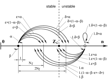
FIG. 1.: The Markov chain representing a collection of states (slopes) for any site $x$ in the sand pile model.

FIG. 2.: The SO profiles of gradient of the pile (${Z_{c}}=8,\ {N_{f}}=3$) for three noise levels.

REFERENCES

-
[1]
Also at the Institute for Nuclear Fusion, RRC
“Kurchatov Institute”, Moscow 123182, RUSSIA.
Electronic address: mmedvedev@ucsd.edu,
http://sdphpd.ucsd.edu/~medvedev/mm.html - [2] Also at General Atomics, San Diego, California 92121.
- [3] O. Biham, et. al, Phys. Rev. A 46, R6124 (1992); K. Nagel and M. Paczuski, Phys. Rev. E 51, 2909 (1995).
- [4] S. Vollmar and H. Herrmann, Physica A, 215, 411 (1995); A. Karolyi and J. Kertesz, in Proc. 6th Joint EPS-APS Intl. Conf. Phys. Computing (PC’94), (Lugano, Switzerland, 1994), p. 675.
- [5] P. Bak, C. Tang, and K. Wiesenfeld, Phys. Rev. Lett. 59, 381 (1987); Phys. Rev. A 38, 364 (1988).
- [6] L.P. Kadanoff, et. al, Phys. Rev. A 39, 6524 (1989).
- [7] Markovian dynamics of a sand pile has also been used by A.B. Chhabra, et. al, Phys. Rev. E 47, 3099 (1993).
- [8] T. Hwa and M. Kardar, Phys. Rev. Lett. 62, 1813 (1989); Phys. Rev. A 45, 7002 (1992); D. Dhar and R. Ramaswamy, Phys. Rev. Lett. 63, 1659 (1989); H.M. Jaeger, et. al, Phys. Rev. Lett. 62, 40 (1989).
- [9] A. Vespignani, et. al, Phys. Rev. E 51, 1711 (1995).
- [10] P.H. Diamond,T.S. Hahm, Phys. Plasmas 2, 3640 (1995).
- [11] J.P. Gollub, et. al, Phys. Rev. Lett. 67, 3507 (1991); B.R. Lane, et. al, Phys. Fluids A 5, 2255 (1993); B. Castaing, et. al, J. Fluid Mech. 204, 1 (1989).
- [12] D.E. Newman, et. al, Phys. Lett. A 218, 58 (1996); Phys. Plasmas, 3, 1858 (1996).
- [13] J.M. Carlson, et. al, Phys. Rev. Lett. 65, 2547 (1990).
- [14] D. Dhar, Phys. Rev. Lett. 64, 1613 (1990); S.M. Majumdar and D. Dhar, Physica A 185, 129 (1992).
- [15] V.B. Priezzhev, J. Stat. Phys. 74, 955 (1994); E.V. Ivashkevich, J. Phys. A 27, 3643 (1994).
- [16] E.V. Ivashkevich, et. al, J. Phys. A 27, L585 (1994); E.V. Ivashkevich, Phys. Rev. Lett. 76, 3368 (1996).