Mesoscopic phenomena in Bose-Einstein systems:
Persistent currents, population oscillations and quantal phases

Abstract

Mesoscopic phenomena—including population oscillations and persistent currents driven by quantal phases—are explored theoretically in the context of multiply-connected Bose-Einstein systems composed of trapped alkali-metal gas atoms. These atomic phenomena are bosonic analogues of electronic persistent currents in normal metals and Little-Parks oscillations in superconductors.

PACS numbers: 03.75.Fi, 73.23.Ra, 03.65.Bz, 74.25.Bt

Introduction: The purpose of this Letter is to consider multiply-connected many-particle systems obeying Bose-Einstein statistics and, in particular, to address the sensitivity of such systems to quantal phases. If the bosonic constituents (e.g., alkali-metal gas atoms) are electrically neutral, electromagnetism, in the form of the Aharonov-Bohm (AB) phase, cannot provide a source of quantal phase. Then, in seeking sensitivity to quantal phases we are led to consider the spin degree of freedom of the bosons, and the consequent possibility of quantal phases of geometric origin [1]. As we shall see, geometric quantal phases can readily affect the energy levels, and hence populations, of the single-particle quantum states, and lead to persistent equilibrium currents in multiply-connected systems, thus providing a striking example of quantal mesoscopic phenomena in the setting of bosonic systems. Such phenomena are bosonic analogues of phenomena well known in the context of the mesoscopic physics of normal-state electronic systems (such as persistent equilibrium currents and conductance oscillations in conducting rings) which arise due to AB [2] or geometric [3] quantal phases. They are also bosonic analogues of the flux-sensitivity of the superconducting transition temperature of a thin superconducting ring, known as Little-Parks oscillations [4]. (These quantum interference phenomena are mesoscopic, in the sense that they vanish in the limit of large system-size.)

It is worth mentioning that there is a sense in which bosonic settings are preferable to electronic settings, if one wishes to observe implications of quantal phases in many-particle physics: in the fermionic case, the Pauli exclusion principle forces the occupation of many single-particle states, and there are strong cancellations between the effects of quantal phases on these states. By contrast, Bose-Einstein statistics promote the significance of the single-particle ground state. In this sense then, bosonic systems tend to amplify mesoscopic effects, at least in comparison with fermionic systems.

One scheme for introducing a geometric quantal phase is to have the bosons move through regions of space in which there is a spatially varying magnetic field to which the spins of the bosons are Zeeman-coupled. Then, as discussed in Ref. [5] in the context of magnetic traps, the inhomogeneous magnetic field (if sufficiently strong) leads to a geometric vector potential ${\bf A}$ (and a corresponding geometric flux $\Phi$) which influences the orbital motion of the bosons, and does so in much the same way as the electromagnetic (AB) vector potential (and flux) influences the motion of electrically charged particles.

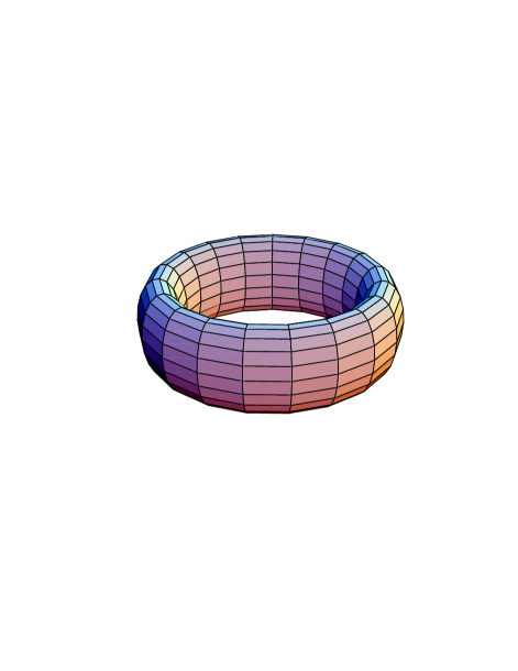
FIG. 1.: Toroidal sample of non-circular cross-section.

References [5] considered conventional (i.e., not AB-like) consequences of the geometric vector potential, i.e., effects associated with nonzero values of the geometric field-strength ${\bf\Omega}\equiv{\bf\nabla}\times{\bf A}$ (i.e., the vorticity). However—and this is the main point of the present Letter—there are striking quantal AB-like consequences of the geometric vector potential itself (rather than the field-strength), especially in multiply-connected configurations, and even when ${\bf\Omega}={\bf 0}$ in the sample. These consequences include an oscillatory dependence on the geometric flux $\Phi$ of the energies of all single-particle levels and, thus, the equilibrium populations of these levels and, more generally, all equilibrium quantities. Moreover, these single-particle energy-level oscillations lead directly to the existence of equilibrium currents [6] that flow around the trap (at generic values of $\Phi$). Therefore, despite the electrical neutrality of the atoms in BEC systems, the geometric phase allows one to realize counterparts of the well-established collection of electromagnetic AB-phase sensitive phenomena, as well as new, bosonic, phenomena such as large oscillations in the populations of the various single-particle levels.

In order to realize geometric-phase–driven oscillations one needs to vary the inhomogeneous magnetic field [7] that the bosons inhabit. In magnetic traps, the ability to make such variations is limited, as variations alter the structure of the trap (i.e., the shape of the system). The recent achievement of confinement via purely optical traps [8] liberates the magnetic field from its dual role of confining the atoms and causing the geometric phase, and thus enlarges the scope for exploring the effects of geometric phases. We shall touch upon the issue of making multiply-connected traps at the end of this Letter.

Model system: We consider a system of many identical charge-neutral noninterating bosonic atoms of mass $m$, confined to a multiply-connected trap. For the sake of simplicity, we envisage the trap as having the following features: (i) it is toroidal and axisymmetric; (ii) it is sufficiently narrow in the radial direction that, under operating conditions, only the state with the lowest radial quantum number is occupied (i.e., the radial energy scale $\hbar\Omega_{r}$ is large); (iii) in the axial direction there is confinement by an oscillator potential; and (iv) if the trap is optical then only mild conditions need be obeyed if an applied inhomogeneous magnetic field is not to change the trapping potential appreciably. (v) If the trap is magnetic then the application of an additional homogeneous field will change $\Phi$ but not the confining potential. In the absence of $\Phi$, the spectrum of single-particle energy eigenvalues ${\cal E}_{\ell,n}^{0}$ is given by ${\cal E}_{\ell,n}^{0}=\hbar\Omega_{z}\,n+\hbar\Omega_{\phi}\,\ell^{2}$, where $\hbar\Omega_{z}$ is the axial oscillator energy scale, $\hbar\Omega_{\phi}$ is the azimuthal energy scale, we have omitted all zero-point energy contributions, and we do not allow for radial excitation. The quantum numbers $\ell$ and $n$ range, respectively, over all integers and all non-negative integers.

We now suppose that the toroidal system of trapped atoms is subjected to a magnetic field having the property that the orientation of the field varies across the trap [9]. Under conditions of adiabaticity (i.e., $\Omega_{\phi}$ much smaller than the Larmor frequency of the spins) for the dynamics of the spins of the atoms, the dominant effect of the inhomogeneous magnetic field on the energy spectrum is to introduce a spin-dependent flux $\Phi$, so that the spectrum (for atoms with spin-projection lying parallel to the magnetic field) becomes

$${\cal E}_{\ell,n}=\hbar\Omega_{z}\,n+\hbar\Omega_{\phi}\,(\ell-\Phi)^{2}.$$ (1)

(Atoms with spin-projection lying antiparallel to the magnetic field direction are not trapped.)   The origin of this flux is the Berry phase associated with the spin dynamics (see, e.g., Refs. [3]). Our aim is to compute the number of particles in the single-particle ground state as a function of the temperature $T$, the geometric flux $\Phi$, and the mean total number of particles $N$, and to do so via the grand canonical ensemble [10]. To this end, we first compute the total number of particles $N$, as a function of $T$, $\Phi$ and the chemical potential $\mu$:

$$N(T,\Phi,\mu) = \sum\nolimits_{\ell=-\infty}^{\infty}\sum\nolimits_{n=0}^{\infty}N_{\ell,n},$$ (3)

$$N_{\ell,n} \equiv \big{\{}{\rm e}^{({\cal E}_{\ell,n}-\mu)/k_{\rm B}T}-1\big{\}}^{-1}.$$ (4)

Next, we decompose this sum: $N=\tilde{N}+\hat{N}$, where

$$\tilde{N}\equiv\sum\nolimits_{\ell=-\infty}^{\infty}N_{\ell,0},\quad\hat{N}\equiv\sum\nolimits_{\ell=-\infty}^{\infty}\sum\nolimits_{n=1}^{\infty}N_{\ell,n}.$$ (5)

To compute $\tilde{N}$, we use a variant of the contour integration technique described, e.g., in Refs. [11], which yields

$$\tilde{N} = {\pi\over{2\varphi}}\left\{\cot\pi\left(\Phi-\varphi\right)-\cot\pi\left(\Phi+\varphi\right)\right\}$$ (7)

$$\qquad\qquad\qquad+{\cal O}\Big{(}\exp\left(-(2\pi)^{3/2}/\tilde{\Omega}_{\phi}^{1/2}\right)\Big{)},$$

where we have introduced the reduced frequency $\tilde{\Omega}_{\phi}\equiv\hbar\Omega_{\phi}/k_{\rm B}T$, and the reduced chemical potential $\tilde{\mu}\equiv\mu/k_{\rm B}T$ and, for convenience, $\varphi$ denotes $\big{(}{\tilde{\mu}/\tilde{\Omega}_{\phi}}\big{)}{{}^{1/2}}$. [The form for $\tilde{N}$ arrived at by this technique is much more rapidly convergent than the original form, Eq. (3)]. Not surprisingly, however, even after omitting exponentially small terms, the transcendental equation for $\tilde{\mu}(T,\Phi,\tilde{N})$, Eq. (7), cannot, in general, be solved explicitly. Without loss of generality, let us assume that $0\leq\Phi\leq 1/2$. (Results for other values of $\Phi$ can be obtained via the symmetries of reflection, $\Phi\to-\Phi$, and translation, $\Phi\to\Phi+1$.) Then further simplification is achievable in three cases: (i) $\Phi\ll 1/2$, (ii) $\Phi\gg\big{(}{\tilde{N}\tilde{\Omega}_{\phi}}\big{)}{{}^{-1/2}}$, and (iii) $|\cot 2\pi\Phi|\gg\tilde{N}\tilde{\Omega}_{\phi}\Phi/\pi$. In case (i) we expand the cotangents on the r.h.s of Eq. (7) in Laurent series, retaining two terms in each series, and solve the resulting equation for $\tilde{\mu}$, thus arriving at

$$\tilde{\mu}\approx\tilde{\Omega}_{\phi}\Phi^{2}-\{\tilde{N}-\big{(}\pi/3\tilde{\Omega}_{\phi}\big{)}\}^{-1}.$$ (8)

In case (ii) we instead expand the prefactor and the arguments of the cotangents in Eq. (7) to linear order in the deviation of $\tilde{\mu}$ from the (dimensionless) single-particle ground-state energy $\tilde{\Omega}_{\phi}\Phi^{2}$. Thus, we arrive at

$$\tilde{\mu} \approx \tilde{\Omega}_{\phi}\Phi^{2}-2\pi^{-1}\Phi\,{\rm cot}^{-1}\Big{(}\cot 2\pi\Phi+\pi^{-1}\Phi\tilde{\Omega}_{\phi}\tilde{N}$$ (10)

$$\qquad\qquad+\sqrt{\cot^{2}\pi\Phi+(\Phi\tilde{\Omega}_{\phi}\tilde{N}/\pi)^{2}+1}\,\,\Big{)}.$$

In case (iii), which corresponds to $\Phi$ close to 1/2, we have

$$\tilde{\mu}\approx\tilde{\Omega}_{\phi}\Phi^{2}-2\pi^{-1}\Phi\,{\rm cot}^{-1}\big{(}\Phi\tilde{\Omega}_{\phi}\tilde{N}/\pi\big{)}.$$ (11)

In making our expansions of Eq. (7) for $\tilde{N}$ we restrict ourselves to the regime of quasi-BEC, i.e., we consider values of $\mu$ only slightly smaller than the single-particle ground-state energy ${\cal E}_{0,0}$ (i.e., $\hbar\Omega_{\phi}\Phi^{2}$).

Physical consequences of the geometric flux: To use these results for $\tilde{\mu}(T,\Phi,\tilde{N})$ to determine desired physical quantities, such as the populations $N_{\ell,n}$ of the single-particle states as functions of the variables $(T,\Phi,N)$, we first note that in the regime of BEC we need only retain the difference between $\mu$ and ${\cal E}_{0,0}$ in $\tilde{N}$, but may omit

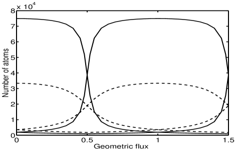
FIG. 2.: Oscillatory dependence on the geometric flux of the populations of the lowest three single-particle energy levels at a higher (dashed line) and a lower (full line) temperature.

it from $\hat{N}$. Next, we observe that $N\equiv\tilde{N}+\hat{N}$, so that by knowing $\tilde{\mu}(T,\Phi,\tilde{N})$ we know $\tilde{\mu}(T,\Phi,N)$. This we use to eliminate $\mu$ from the Bose functions that determine the populations $N_{\ell,n}$. To illustrate the oscillatory behavior of single-particle state populations with $\Phi$ we show, in Fig. 2, the populations $N_{\ell,m}$ of the three lowest-lying states (i.e., $N_{0,0}$, $N_{1,0}$ and $N_{2,0}$, as $|\Phi|\leq 1/2$) as functions of $\Phi$ [12]. We have chosen for this illustration a system of $N=10^{5}$ atoms of ⁸⁷Rb, sample radius $R=1\,\mu{\rm m}$, axial trap frequency $\Omega_{z}=7,500\,{\rm Hz}$, temperature $T=5\,\mu{\rm K}$ (for which $800\tilde{\Omega}_{\phi}=40\tilde{\Omega}_{z}=1$) or $T=10\,\mu{\rm K}$ (for which $400\tilde{\Omega}_{\phi}=20\tilde{\Omega}_{z}=1$), where $\tilde{\Omega}_{z}{\equiv}\hbar\Omega_{z}/k_{\rm B}T$. Note that at $\Phi{=}0$ we have $N_{\ell,n}{=}N_{-\ell n}$, and at $\Phi{=}1/2$ we have $N_{\ell,n}{=}N_{\ell+1,n}$. The latter case illustrates the more general point that at half-integral values of $\Phi$ the lowest single-particle energy level is degenerate for the case of perfectly azimuthally symmetric traps. If, however, the azimuthal symmetry is absent then the level crossing is avoided, and the single-particle ground state is separated from the excited states by an energy gap at all values of $\Phi$.

The population oscillations are mesoscopic, in the sense that they vanish in the thermodynamic limit [13]. Indeed, the number of atoms in traps, although typically large, is not on the order of Avogadro’s number and, therefore, the systems are even further from the thermodynamic limit than conventional macroscopic and even mesoscopic samples. Nevertheless, although BEC is not, strictly speaking, marked by a sharp thermodynamic phase transition, atomic condensates acquire features of the thermodynamic limit already at $N=10^{4}$ (see, e.g., Refs. [14, 15]). Despite this, our calculations reveal oscillatory phenomena at $N=10^{5}$ whenever the fraction of atoms in the ground state is appreciable. Thus, one has the capability of observing, simultaneously, both macroscopic and mesoscopic phenomena.

The $\Phi$-dependence of the single-particle energy levels also leads to the phenomenon of equilibrium persistent currents, i.e., dissipationless particle-currents that flow around the trap. (Such equilibrium currents should, of course, be distinguished from the nonequilibrium metastable currents that can arise in multiply-connected samples; see, e.g., Refs. [6].)  The simple formula,

$$I=\sum\nolimits_{\ell=-\infty}^{\infty}\sum\nolimits_{n=0}^{\infty}N_{\ell,n}\,\partial{\cal E}_{\ell,n}/\partial\Phi,$$ (12)

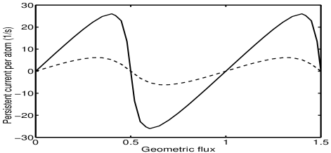
FIG. 3.: Oscillatory dependence of the equilibrium persistent particle-current (per atom) on the geometric flux at a higher (dashed line) and a lower (full line) temperature.

for the persistent particle-current $I$ follows from the general relation $\delta F/\delta{\bf A}=-{\bf j}$, where $F$ is the free energy, ${\bf A}$ is a gauge potential (such as the geometric vector potential) and ${\bf j}$ is the conjugate current-density. In Fig. 3 we show the dependence of $I/N$ on $\Phi$ at the conditions and temperatures specified in the previous paragraph. As $T$ is increased from zero the saw-tooth form of the $\Phi$-dependence is smoothed to a more sinusoidal form, but the zeros at integral and half-integral values of the flux are preserved. As for the characteristic scale of the amplitude of $I$, it is on the order of $N\Omega_{\phi}$, at least when the ground state contains most of the particles.

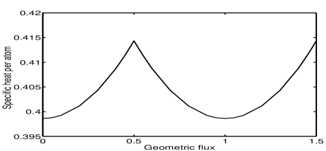
FIG. 4.: Oscillatory dependence of the specific heat per atom on the geometric flux.

As it is Fermi rather than Bose systems that have traditionally provided settings for mesoscopic physics, we pause to compare the characteristic magnitudes of persistent currents in Fermi and Bose systems. In the special case of single-channel systems the characteristic magnitudes are similar: the many bosons in the (low-velocity) ground state contributing roughly as much as the single (high-velocity) fermion at the Fermi level (contributions from fermions below the Fermi level essentially cancelling one another). In the more general case, however, in which there are many channels, the greater the extent of transverse excitation, the smaller the contribution to the persistent fermion current (owing to the reduced kinetic energy at the Fermi level). By contrast, for bosons the particle occupations are, of course, not spread over the many current-reduced channels, and instead are concentrated on the optimal channel. Thus, for bosonic systems such mesoscopic effects are amplified, relative to the Fermi case.

As a third consequence of the geometric flux, we consider the oscillatory behavior of the (dimensionless) specific heat (per particle) $C\equiv\partial E(T,\Phi,N)/\partial Nk_{\rm B}T$. (We recognize that $C$ may be difficult to measure.)   For $C$, a more pronounced $\Phi$-dependence arises in the case of traps that are weakly confining in the axial direction (i.e., $\Omega_{z}\ll\Omega_{\phi}$). In Fig. 4 we show $C(\Phi)$ for the case of ²³Na (the reduced mass of which also enhances the sensitivity to $\Phi$ compared with ⁸⁷Rb) at $R=0.5\,\mu{\rm m}$, $T=40\,{\rm nK}$ and $\Omega_{z}=100\,{\rm Hz}$. Upon closer inspection, the apparent cusp at the level crossing, which is a remnant of the true singularity at $T=0$, is seen to be rounded.

Experimental issues and concluding remarks: Having described several consequences of the geometric flux, we now briefly discuss some issues concerning the possibility of the experimental realization of these consequences. We see three pivotal matters: (i) how to construct a toroidal sample; (ii) how to subject the sample to a suitably inhomogeneous field; and (iii) how to detect population oscillations and persistent currents. As for (i), it should be feasible to construct toroidal samples based on magnetic traps by using a blue-detuned laser to repel atoms from the trap center. We hope that in purely optical traps [8] a similar method, combining red- and blue-detuned lasers, could be employed to make a toroidal sample. As for (ii), magnetic trap technology itself is suitable for creating the necessary textured magnetic fields. (As magnetic traps are currently used as a first stage in the loading of optical traps, creating textured fields should not impose a large additional experimental burden.)  As for (iii), the phonon-imaging technique [16] discussed with regard to metastable currents in the last paragraph of the second of Refs. [6] is less difficult in the present setting of equilibrium persistent currents, owing to the far larger magnitude of the latter. Other experimental possibilities may include (nondestructive) light-scattering and (destructive) time-of-flight techniques.

We note that interactions between the bosons are not expected to alter qualitatively the oscillatory effects that we have discussed. This is because, in the present context, $k_{\rm B}T\gg\mu$, for which one expects interactions to have only perturbative consequences [15]. We conclude by remarking that if it is possible to realize superconductivity via the BEC of pre-formed bosons then oscillations in the level-populations, persistent currents, and perhaps specific heat, similar to those described in the present Letter, may be observable as consequences of an AB flux.

Useful discussions with A. Balaeff, C. Bender, A. J. Leggett and the UIUC/CNRS Bose-Einstein Condensation Workshop participants are gratefully acknowledged. This work was supported by the Department of Energy, Division of Materials Sciences, Grant DEFG02-96ER45439.

REFERENCES

- [1] M. V. Berry, Proc. R. Soc. London A 392, 45 (1984).
- [2] A. G. Aronov and Yu. V. Sharvin, Rev. Mod. Phys. 59, 755 (1987).
- [3] See, e.g., D. Loss, P. M. Goldbart and A. V. Balatsky, Phys. Rev. Lett. 65, 1655 (1990); A. Stern, ibid. 68, 1022 (1992); D. Loss, H. Schoeller and P. M. Goldbart, Phys. Rev. B 48, 15218 (1993); Y. Lyanda-Geller, I. L. Aleiner and P. M. Goldbart, Phys. Rev. Lett. 81, 3215 (1998).
- [4] W. A. Little, R. D. Parks, Phys. Rev. Lett. 9, 9 (1962).
- [5] T.-L. Ho and V. B. Shenoy, Phys. Rev. Lett. 77, 2595 (1996); see also T.-L. Ho, cond-mat/9803231.
- [6] Recently, certain nonequilibrium properties of BEC in toroidal traps (e.g., the stability and thermal decay of metastable current-carrying states) were considered in: D. Rokhsar, cond-mat/9709212; E. Mueller, P. Goldbart and Y. Lyanda-Geller, Phys. Rev. A 57, R1505 (1998).
- [7] Recently, K. G. Petrosyan and L. You [cond-mat/ 9810059] proposed a scheme for observing the Aharonov-Casher effect in BEC systems, the origin of this effect being a radial electric field passing through a toroidal sample. This scheme had previously been proposed in the context of superfluid 3He in A. V. Balatsky and B. L. Altshuler, Phys. Rev. Lett. 70, 1678 (1993).
- [8] D. Stamper-Kurn et al., Phys. Rev. Lett. 80, 2027 (1998).
- [9] In optical traps one can use Helmholtz coils to create radial fields. By adding a homogeneous field one can create, e.g., crown-shaped fields.
- [10] Although it seems more appropriate to use the canonical (i.e., fixed particle-number) ensemble, it is more straightforward to use the grand-canonical ensemble, as we have done. We hope that the error incurred is negligible, at least at the particle numbers on which we are focusing.
- [11] A. L. Fetter and J. D. Walecka, Quantum theory of many-particle systems (San Francisco, McGraw-Hill, 1971), pp. 248-250; F. Olver, Introduction to Asymptotics and Special Functions (NY, Academic Press, 1973), Sec. 8.
- [12] For this illustration we have computed the populations numerically, using Eqs. (3) and (4).
- [13] By the thermodynamic limit we mean , and , but with tending to a constant. In this limit, we arrive at a system that, although two-dimensional geometrically, does indeed exhibit thermodynamically sharp BEC, owing to the precise form of the density of states associated with the axial oscillator.
- [14] N. J. Van Druten and W. Ketterle, Phys. Rev. Lett. 79, 549 (1997).
- [15] F. Dalfovo, S. Giorgini, L. P. Pitaevskii and S. Stringari, Rev. Mod. Phys. (in press, 1998); cond-mat/9806038.
- [16] M. R. Andrew et al., Phys. Rev. Lett. 79, 553 (1997).