[

Positional Disorder (Random Gaussian Phase Shifts) in the Fully Frustrated Josephson Junction Array (2D XY Model)

Abstract

We consider the effect of positional disorder on a Josephson junction array with an applied magnetic field of $f=1/2$ flux quantum per unit cell. This is equivalent to the problem of random Gaussian phase shifts in the fully frustrated 2D XY model. Using simple analytical arguments and numerical simulations, we present evidence that the ground state vortex lattice of the pure model becomes disordered, in the thermodynamic limit, by any finite amount of positional disorder.

]

The stability of vortex lattices to random disorder is a topic of considerable recent interest, motivated by studies of the high temperature superconductors. In two dimensions (2D), periodic arrays of Josephson junctions form a well controlled system for investigating similar issues of vortex fluctuations and disorder. Here we consider the effect of “positional” disorder on the vortex lattice of the fully frustrated Josephson array, with $f=1/2$ flux quantum of applied magnetic field per unit cell.

Positional disorder [2, 3, 4, 5] was first discussed with respect to the Kosterlitz-Thouless (KT) transition for the $f=0$ model in zero magnetic field. Early arguments [2] predicting a reentrant normal phase at low temperatures have been revised by recent works [3, 5] which argue that there is a finite critical disorder strength $\sigma_{c}\simeq\sqrt{\pi/8}$; for $\sigma<\sigma_{c}$ an ordered state persists for $0\leq T\leq T_{c}(\sigma)$. For the pure $f=1/2$ case on a square grid [6, 7], the ordered state has two broken symmetries: the $U(1)$ symmetry (“KT-like” order) associated with superconducting phase coherence, and the $Z(2)$ symmetry (“Ising-like” order) associated with the “checkerboard” vortex lattice, in which a vortex sits on every other site. Previous works [8, 9] have considered the effect of positional disorder on this $f=1/2$ model; all have concluded that both Ising-like and KT-like order persist for at least small disorder strengths $\sigma$. In this work, however, we present new arguments that suggest that, for $f=1/2$, the critical disorder is $\sigma_{c}=0$.

The Hamiltonian for the Josephson array is given by the “frustrated” 2D XY model [7],

$${\cal H}[\theta_{i}]=\sum_{i\mu}U(\theta_{i}-\theta_{i+\hat{\mu}}-A_{i\mu})\enspace,$$ (1)

where $i$ are the sites of a periodic square grid with basis vectors $\hat{\mu}=\hat{x}$, $\hat{y}$, the sum is over all nearest neighbor (n.n.) bonds $\langle i,i+\hat{\mu}\rangle$ and $\theta_{i}-\theta_{i+\hat{\mu}}-A_{i\mu}$ is the gauge invariant phase difference across the bond, with $A_{i\mu}=(\phi_{0}/2\pi)\int_{i}^{i+\hat{\mu}}{\bf A}\cdot d\ell$ the integral of the vector potential.

Positional disorder arises from random geometric distortions of the bonds of the grid, resulting in, $A_{i\mu}=A_{i\mu}^{(0)}+\delta A_{i\mu}$; $A_{i\mu}^{(0)}$ is the value in the absence of disorder, and $\delta A_{i\mu}$ is the random deviation. We take the $\delta A_{i\mu}$ to be independent Gaussian random variables with

$$[\delta A_{i\mu}]=0,\quad{\rm and}\quad[\delta A_{i\mu}\delta A_{j\nu}]=\sigma^{2}\delta_{ij}\delta{\mu\nu}\enspace.$$ (2)

$[\ldots]$ denotes an average over the quenched disorder. The positionally disordered array is thus also referred to as the XY model with random Gaussian phase shifts.

When $U(\phi)$ is the Villain function [10], the Hamiltonian (1) is equivalent to a dual “Coulomb gas” of interacting vortices [6, 11, 12],

$${\cal H}[n_{i}]={1\over 2}\sum_{ij}(n_{i}-f-\delta f_{i})G_{ij}(n_{j}-f-\delta f_{j})\enspace.$$ (3)

The sum is over all pairs of dual sites $i$, $j$, $n_{i}$ is the integer vorticity on site $i$, and the interaction $G_{ij}$ is the Green’s function for the 2D discrete Laplacian operator, $\Delta_{ik}G_{kj}=-2\pi\delta_{ij}$, where $\Delta_{ij}\equiv\delta_{i,j+\hat{x}}+\delta_{i,j-\hat{x}}+\delta_{i,j+\hat{y}}+\delta_{i,j-\hat{y}}-4\delta_{ij}$. For large separations, $G_{ij}\simeq-\ln|{\bf r}_{i}-{\bf r}_{j}|$. The $f_{i}\equiv f+\delta f_{i}$ are $(1/2\pi)$ times the circulation of the $A_{i\mu}$ around dual site $i$; $f$ is the average applied flux, while $\delta f_{i}$ is the deviation due to the random $\delta A_{i\mu}$,

$$\delta f_{i}={1\over 2\pi}\left[\delta A_{i,x}+\delta A_{i+\hat{x},y}-\delta A_{i+\hat{y},x}-\delta A_{i,y}\right]\enspace.$$ (4)

Geometrically distorting a bond increases the flux through the cell on one side of the bond, while reducing the flux through the cell on the opposite side by the same amount. The $\delta f_{i}$ are thus anticorrelated among n.n. sites. Positional disorder is thus the same as random dipole pairs of quenched charges $\pm\delta f_{i}$ [2]. From Eqs. (2) and (4) we get,

$$[\delta f_{i}]=0,\quad{\rm and}\quad[\delta f_{i}\delta f_{j}]=-{\sigma^{2}\over 4\pi^{2}}\Delta_{ij}\enspace.$$ (5)

The Hamiltonian (3) can be rewritten as interacting charges in a one body random potential [3],

$${\cal H}[q_{i}]={1\over 2}\sum_{ij}q_{i}G_{ij}q_{j}-\sum_{i}q_{i}V_{i}\enspace,$$ (6)

where $q_{i}\equiv n_{i}-f$, and the random potential is $V_{i}=\sum_{j}G_{ij}\delta f_{j}$. For $f=1/2$, $q_{i}=\pm 1/2$. From Eq. (5),

$$[V_{i}]=0, {\rm and}\quad[V_{i}V_{j}]=\sum_{k,l}G_{ik}[\delta f_{k}\delta f_{l}]G_{lj}$$ (7)

$$= -{\sigma^{2}\over 4\pi^{2}}\sum_{k,l}G_{ik}\Delta_{kl}G_{lj}={\sigma^{2}\over 2\pi}G_{ij}\enspace,$$ (8)

The $V_{i}$ thus have logarithmic long range correlations.

We now use an Imry-Ma [13] type argument to estimate the stability of the doubly degenerate checkerboard ground state to the formation of a square domain of side $L$. The energy of such an excitation consists of a domain wall term, $E_{d}$, which is present for the pure case, and a pinning term, $E_{p}$, due to the interaction with the random $V_{i}$. $E_{d}(L)$ has the form [14],

$$E_{d}\simeq aL+c\ln L+d\enspace.$$ (9)

The first term is the interfacial tension of the domain wall; the second term comes from net charge that builds up at the corners of the domain [15]. Calculating $E_{d}(L)$ numerically for a pure system, we find an excellent fit to Eq. (9), with $a=0.28$, $c=0.15$, and $d=0.058$.

By Eq. (8), the average pinning energy of the domain ${\cal D}$, $[E_{p}]=2\sum_{i\in{\cal D}}q_{i}[V_{i}]=0$, but the variance is,

$$[E_{p}^{2}]=4\sum_{i,j\in{\cal D}}q_{i}[V_{i}V_{j}]q_{j}={4\sigma^{2}\over 2\pi}\sum_{i,j\in{\cal D}}q_{i}G_{ij}q_{j}={4\sigma^{2}\over\pi}E_{0}\enspace,$$ (10)

where $E_{0}=(\pi/32)L^{2}$ is the ground state energy of the checkerboard domain [16]. The root mean square pinning energy is thus,

$$[E_{p}]_{rms}=bL,\quad b={\sigma\over 2\sqrt{2}}\simeq 0.35\sigma\enspace.$$ (11)

For domains whose energy is lowered by the interaction with $V_{i}$, the typical excitation energy is $E=E_{d}-[E_{p}]_{rms}$. Eqs. (9) and (11) imply that when $b>a$, i.e. when $\sigma>\sigma_{c}\simeq 0.8$, $E(L)$ has a maximum at $L=\xi\equiv(c/2\sqrt{2})/(\sigma-\sigma_{c})$. Domains of size $L>\xi$ will lower their energy by increasing in size, and so disorder the system. Thus, one naively expects that when $\sigma<\sigma_{c}$ the system preserves its Ising-like order, but when $\sigma>\sigma_{c}$ the system is disordered into domains of typical size $\xi$.

However the leading size dependencies of Eqs. (9) and (11), $E_{d}\sim[E_{p}]_{rms}\sim L$, are exactly the same as found in the 2D n.n. random field Ising model (RFIM). For the RFIM it is known [13, 17, 18] that 2D is the lower critical dimension, that the randomness causes domains walls at $T=0$ always to roughen and so acquire an effective negative line tension, and that the critical disorder is $\sigma_{c}=0$, i.e. any amount of disorder, no matter how weak, destroys the Ising-like order of the pure case. By analogy, we suggest that the positionally disordered $f=1/2$ 2D XY model similarly has $\sigma_{c}=0$. Our conclusion, that $[E_{p}]_{rms}\sim L$ as in the 2D RFIM, follows from a subtle cancellation between the long range interactions between charges $q_{i}$, and the long range correlations of the random potential $V_{i}$.

To check this prediction, we carry out Monte Carlo (MC) simulations of the Hamiltonian (3) with periodic boundary conditions on $L\times L$ square grids. Our MC procedure is as follows [16]. One MC excitation attempt consists of the insertion of a neutral $n=\pm 1$ vortex pair on n.n. or next n.n. sites, which is accepted or rejected using the usual Metropolis algorithm. $L^{2}$ such attempts we call one MC pass. At each temperature we typically used $4000$ MC passes to equilibrate the system, followed by $128,000$ MC passes to compute averages. Every $100$ passes we attempt a global excitation reversing the sign of all the charges, $q_{i}\to-q_{i}$. For each disorder realization we cooled down two distinct “replicas”, starting with different random charge configurations and using different random number sequences. In only about $3\%$ of the cases did the two replicas fail to give reasonable agreement.

To test for Ising-like order we define an order parameter analogously to an Ising antiferromagnet,

$$M={1\over L^{2}}\sum_{i}q_{i}(-1)^{x_{i}+y_{i}}\enspace.$$ (12)

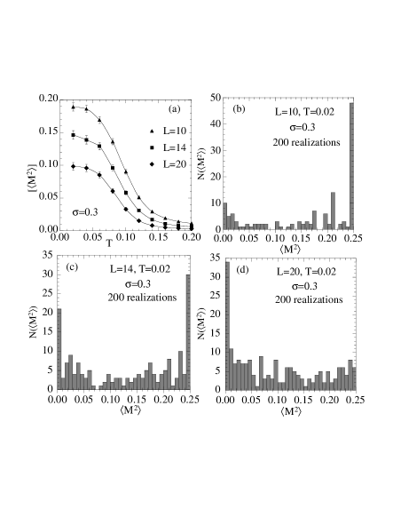
FIG. 1.: (a) $[\langle M^{2}\rangle]$ vs. $T$, for $\sigma=0.3$, and sizes $L=10$, $14$, $20$ (solid lines are guides to the eye); Histogram of occurrences of $\langle M^{2}\rangle$ in $200$ realizations of disorder, for $\sigma=0.3$ at low $T=0.02$, for (b) $L=10$, (c) $L=14$ and (d) $L=20$.

We first consider $\sigma=0.3$, smaller than both the naive estimate of $\sigma_{c}=0.8$, and the $\sigma_{c}=\sqrt{\pi/8}\simeq 0.63$ of the $f=0$ model. Fig. 1 plots $[\langle M^{2}\rangle]$ vs. $T$, averaged over $200$ disorder realizations, for sizes $L=10$, $14$ and $20$. All curves start to increase from zero near $T\simeq 0.13$, which is $T_{c}(\sigma=0)$ of the pure model. However $[\langle M^{2}\rangle]$ at low $T$ decreases steadily with increasing $L$. The reason for this becomes clearer if we consider the histogram of values of $\langle M^{2}\rangle$ that occur as we sample the different realizations of disorder. We show such histograms in Figs. 1b-d, for the lowest temperature $T=0.02$. As $L$ increases, the statistical weight shifts from predominantly ordered systems ($M^{2}=1/4$), to predominantly disordered systems ($M^{2}=0$). Assuming that this trend continues, we expect that as $L\to\infty$, $[\langle M^{2}\rangle]\to 0$.

To measure the “random field correlation length” $\xi$, we consider the vortex correlation function,

$$S({\bf k})={1\over L^{2}}\sum_{i,j}e^{i{\bf k}\cdot({\bf r}_{i}-{\bf r}_{j})}\langle n_{i}n_{j}\rangle\enspace.$$ (13)

For the pure case, $S({\bf k})$ in the ordered phase has singular Bragg peaks at ${\bf K}=\pm\pi\hat{x}\pm\pi\hat{y}$. If the vortex lattice is disordered, these peaks will broaden, and their finite width provides a measure of $\xi$. Writing ${\bf k}={\bf K}+\delta{\bf k}$, and assuming a Lorentzian shape for the disorder averaged peak, $[S({\bf k})]\propto 1/(\delta k^{2}+\xi^{-2})$, we determine $\xi$ by fitting to this form for $\delta k=0$, and $\delta k=2\pi/L$ [19]. In Fig. 2 we show $\xi$ vs. $\sigma$ at our lowest $T=0.02$, for several system sizes $L$. Only for our smallest value $\sigma=0.25$ does a finite size effect remain. In this case, however, $\xi$ decreases as $L$ increases. This is in contrast to the increase of $\xi$ with $L$ that one would expect if one were approaching a second order transition. This behavior is consistent with that seen in Figs. 1b-d, where as $L$ increases, a greater fraction of the disorder realizations result in disordered states.

FIG. 2.: Correlation length $\xi(\sigma)$ vs. $\sigma$ at $T=0.02$ for various sizes $L$. Sizes $L=14,20$ are averaged over $200$ realizations of the randomness; sizes $L=30,40$ are averaged over $50$ realizations. Dashed, dotted and solid lines are fits to the scaling forms (i), (ii) and (iii) respectively.

We next fit our results for $\xi(\sigma)$ to several possible scaling expressions: (i) $\xi\sim e^{C/(\sigma-\sigma_{c})^{2}}$, (ii) $\xi\sim e^{C/(\sigma-\sigma_{c})}$, and (iii) $\xi\sim|\sigma-\sigma_{c}|^{-p}$. The first has been suggested by Binder [17] for the 2D RFIM. While in Binder’s expression $\sigma_{c}=0$, here we leave it as an arbitrary parameter to be determined from the fit. The second has been suggested for the positionally disordered $f=0$ model [2, 3], in which $\sigma_{c}>0$. The third is the familiar power law form. Using data for only the largest $L$ for each $\sigma$, the results of these fits are shown in Fig. 2. The value of $\sigma_{c}$ and the $\chi^{2}$ of the fit for each case is (i) $\sigma_{c}=0.0046\pm 0.050$, $\chi^{2}=67$;(ii) $\sigma_{c}=0.0134\pm 0.055$, $\chi^{2}=67$; (iii) $\sigma_{c}=0.0013\pm 0.098$, $p=2.86\pm 0.84$, $\chi^{2}=7.6$. The power law (iii) gives a significantly better fit than (i) or (ii), however all give $\sigma_{c}=0$ within the estimated error. Given the rather limited range of the data, the above fits should be treated with caution. However they do indicate that the data contains no suggestion of a diverging $\xi$ at a finite $\sigma$. Coupled with our Imry-Ma argument, we thus find a consistent picture suggesting that $\sigma_{c}=0$ for the $f=1/2$ 2D XY model.

FIG. 3.: (a) Overlaps $[Q_{\rm self\,1}]$, $[Q_{\rm self\,2}]$, and $[Q_{\rm cross}]$ vs. $T$ for $\sigma=0.3$ and $L=20$; (b) Overlap susceptibility $\chi_{Q}$ vs. $T$ for $\sigma=0.3$ and $L=10$, $14$, $20$. Both are averaged over $200$ disorder realizations.

Returning to the case $\sigma=0.3$, where Ising-like order has been lost, we now consider whether the system may still have a finite temperature “spin glass” transition to a disordered but frozen vortex state. To test for this we measure the self and cross overlaps [20], $Q_{\rm self}$ and $Q_{\rm cross}$,

$$Q_{\rm self\,\alpha} = {1\over L^{2}}\sum_{i}\langle n_{i}^{(\alpha)}(t)n_{i}^{(\alpha)}(t+\tau)\rangle$$ (14)

$$Q_{\rm cross} = {1\over L^{2}}\sum_{i}\langle n_{i}^{(\alpha)}(t)n_{i}^{(\beta)}(t)\rangle\enspace.$$ (15)

$\alpha$ and $\beta$ index the two independent replicas. For $\tau$ sufficiently large we expect $Q_{\rm self\,1}=Q_{\rm self\,2}=Q_{\rm cross}$, if the system is well equilibrated. Averaging Eq. (15) over several values of $\tau\geq 2000$ to improve our statistics, we plot $[Q_{\rm self\,1}]$, $[Q_{\rm self\,2}]$ and $[Q_{\rm cross}]$ vs. $T$ in Fig. 3a. We see that our system is fairly well equilibrated down to the lowest $T$ we study. To test for a spin glass transition, we measure the overlap susceptibility,

$$\chi_{Q}=L^{2}\left\{[\langle Q_{\rm cross}^{2}\rangle]-[\langle Q_{\rm cross}\rangle^{2}]\right\}\enspace,$$ (16)

which we plot vs. $T$ in Fig. 3b for various system sizes. The peak in $\chi_{Q}$ near $T\simeq 0.06$ shows no noticeable increase as $L$ increases, thus suggesting that there is no finite temperature spin glass transition.

If the vortices are not frozen, but are free to diffuse, one expects that superconducting phase coherence is also destroyed. To explicitly test this we measure the helicity modulus. The Hamiltonian (3) can viewed as representing the XY model with “fluctuating twist” boundary conditions [12]. Using the method of Ref. [21], we determine the dependence of the total free energy $F$ of the corresponding XY model, as a function of the twist $(\Delta_{x},\Delta_{y})$ which is applied in a “fixed twist” boundary condition. We then determine the $(\Delta_{x0},\Delta_{y0})$ that minimizes $F$; the helicity modulus tensor is then the curvature of $F$ at the minimizing twist, $\Upsilon_{\mu\nu}=\partial^{2}F/\partial\Delta_{\mu}\partial\Delta_{\nu}$. In Fig. 4a we plot $\Upsilon_{1}$, the largest of the two eigenvalues of $\Upsilon_{\mu\nu}$, vs. $T$, for $\sigma=0.3$ and sizes $L=10,14,20$. At all $T$, $\Upsilon_{1}$ continues to decrease as $L$ increases, giving no suggestion of a finite temperature transition. In Figs. 4b-d we plot histograms of the minimizing twist $\Delta_{0}$ for the three sizes $L$. Note, in choosing our random phase shifts $\delta A_{i\mu}$, we impose the constraint $\sum_{i}\delta A_{i\mu}=0$ in order to remove one trivial source of $\Delta_{0}\neq 0$. We see that the width of the distributions of $\Delta_{0}$ steadily increases with increasing $L$, suggesting [5] that the strength of the random disorder is renormalizing to greater values on larger length scales.

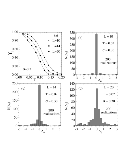
FIG. 4.: (a) $\Upsilon_{1}$ vs. $T$, for $\sigma=0.3$, and sizes $L=10$, $14$, $20$ (solid lines are guides to the eye); Histogram of values of $\Delta_{0}$ found in $200$ disorder realizations, for $\sigma=0.3$ at low $T=0.02$, at (b) $L=10$, (c) $L=14$, and (d) $L=20$.

To conclude, our results suggest that Ising-like order is destroyed for any finite amount of positional disorder. Further, we found in one specific case that when the Ising-like order vanished, no spin glass order or phase coherence existed either. We speculate that this remains true as well for any finite disorder strength. Although $\sigma_{c}=0$, the finite $\xi(\sigma)$ nevertheless can become extremely large for small values of $\sigma$. When $\xi$ exceeds the size of the experimental or numerical sample, the system will indeed look ordered. We believe this explains previous numerical work on this problem which reported the persistence of Ising-like order at small $\sigma$. In the most recent of these works, Cataudella [9] reports at $\sigma\simeq 0.113$ a finite $T_{c}$ to an Ising-like ordered state. The correlation length exponent that he finds is $\nu\sim 1.7$, clearly different from that of the pure model. Using our scaling form (iii) we can estimate that at this value of $\sigma$, $\xi\sim 120$, much larger than Cataudella’s largest system size of $L=36$. His results may thus be reflecting a cross over region at $L<\xi$, rather than a true transition.

We thank Prof. Y. Shapir for many valuable discussions. This work has been supported by DOE grant DE-FG02-89ER14017.

REFERENCES

- [1] Present address: Department of Physics and Astronomy, McMaster University, Hamilton, Ontario, L8S 4M1 Canada
- [2] E. Granato and J. M. Kosterlitz, Phys. Rev. B 33, 6533 (1986); M. Rubinstein, B. Shraiman and D. R. Nelson, Phys. Rev. B 27, 1800 (1983).
- [3] T. Nattermann, S. Scheidl, S. E. Korshunov and M. S. Li, J. Phys. (France) I 5, 565 (1995); L.-H. Tang, Phys. Rev. B 54, 3350 (1996); S. Scheidl, Phys. Rev. B 55, 457 (1997); M. C. Cha and H. Fertig, Phys. Rev. Lett. 74, 4867 (1995); J. Maucourt and D. R. Grempel, Phys. Rev. B 56, 2572 (1997); Y. Ozeki and H. Nishimori, J. Phys. A 26, 3399 (1993).
- [4] M. G. Forrester, S. P. Benz and C. J. Lobb, Phys. Rev. B 41, 8749 (1990); A. Chakrabarti and C. Dasgupta, Phys. Rev. B 37, 7557 (1988); S. P. Benz, M. G. Forrester, M. Tinkham and C. J. Lobb, Phys. Rev. B 38, 2869 (1988); M. G. Forrester, H. J. Lee, M. Tinkham and C. J. Lobb, Phys. Rev. B 37, 5966 (1988); S. E. Korshunov, Phys. Rev. B 48, 1124 (1993).
- [5] J. M. Kosterlitz and M. Simkin, Phys. Rev. Lett. 79, 1098 (1997).
- [6] J. Villain, J. Phys. C. 10, 1717 and 4793 (1977).
- [7] S. Teitel and C. Jayaprakash, Phys. Rev. B 27, 598 (1983); Phys. Rev. Lett. 51, 1999 (1983).
- [8] E. Granato and J. M. Kosterlitz, Phys. Rev. Lett. 62, 823, (1989); M. Y. Choi, J. S. Chung and D. Stroud, Phys. Rev. B 35, 1669 (1987).
- [9] V. Cataudella, Europhys. Lett. 44, 478 (1998).
- [10] J. Villain, J. Physique 36, 581 (1975).
- [11] E. Fradkin, B. Huberman and S. H. Shenker, Phys. Rev. B 18, 4789 (1978); A. Vallat and H. Beck, Phys. Rev. B 50, 4015 (1994).
- [12] P. Olsson, Phys. Rev. B 52, 4511 (1995).
- [13] Y. Imry and S.-K. Ma, Phys. Rev. Lett. 35, 1399 (1975).
- [14] C. Denniston and C. Tang, Phys. Rev. Lett. 79, 451 (1997) and Phys. Rev. B 58, 6591 (1998).
- [15] T. C. Halsey, J. Phys. C 18, 2437 (1985).
- [16] J.-R. Lee and S. Teitel, Phys. Rev. B 46, 3247 (1992).
- [17] K. Binder, Z. Phys. B 50, 343 (1983).
- [18] M. Aizenman and J. Wehr, Phys. Rev. Lett. 62, 2503 (1989); K. Hui and N. Berker, ibid. 2507.
- [19] P. Olsson, Phys. Rev. B. 55, 3585 (1997).
- [20] R. N. Bhatt and A. P. Young, Phys. Rev. B 37, 5606 (1988).
- [21] P. Gupta, S. Teitel and M. J. P. Gingras, Phys. Rev. Lett. 80, 105 (1998).