To appear, Bras. J. Phys. (1999) BU-CCS-981201 Navier-Stokes Equations for Generalized Thermostatistics

Abstract

Tsallis has proposed a generalization of Boltzmann-Gibbs thermostatistics by introducing a family of generalized nonextensive entropy functionals with a single parameter $q$. These reduce to the extensive Boltzmann-Gibbs form for $q=1$, but a remarkable number of statistical and thermodynamic properties have been shown to be $q$-invariant – that is, valid for any $q$. In this paper, we address the question of whether or not the value of $q$ for a given viscous, incompressible fluid can be ascertained solely by measurement of the fluid’s hydrodynamic properties. We find that the hydrodynamic equations expressing conservation of mass and momentum are $q$-invariant, but that for conservation of energy is not. Moreover, we find that ratios of transport coefficients may also be $q$-dependent. These dependences may therefore be exploited to measure $q$ experimentally.

Keywords: Generalized thermostatistics, Tsallis entropy, Chapman-Enskog expansion, Navier-Stokes equations.

I Introduction

A Motivation and Historical Background

The concept of extensivity is introduced early in most textbooks on thermodynamics and statistical physics. The requirement that the entropy be additive establishes the form of the Boltzmann-Gibbs distribution via a straightforward argument. Recently, Tsallis [1] has proposed a generalization of Boltzmann-Gibbs thermostatistics by introducing a family of generalized entropy functionals with a single parameter $q$. The proposed generalization is best described by the following two axioms:

Axiom 1

The entropy functional associated with a probability distribution $f({\bf z})$ is

$$S_{q}[f]\equiv\frac{k_{B}}{q-1}\int d{\bf z}\;\left\{f({\bf z})-\left[f({\bf z})\right]^{q}\right\}.$$ (1)

Axiom 2

The experimentally measured value of a phase function $g({\bf z})$ is given by the $q$-expectation value,

$$G_{q}[f]\equiv\int d{\bf z}\;\left[f({\bf z})\right]^{q}g({\bf z}).$$ (2)

From the first axiom, we note that $S_{q}[f]$ reduces to the Boltzmann-Gibbs entropy in the limit as $q\rightarrow 1$,

$$S_{1}[f]=\lim_{q\rightarrow 1}\frac{k_{B}}{q-1}\int d{\bf z}\;\left\{f({\bf z})-\left[f({\bf z})\right]^{q}\right\}=-k_{B}\int d{\bf z}\;f({\bf z})\ln f({\bf z}),$$ (3)

so the generalized thermostatistics includes the usual one as a special case. It differs most notably in that fact that neither the entropy $S_{q}[f]$ itself nor the observables $G_{q}[f]$ are extensive thermodynamic variables when $q\neq 1$. In spite of this difference, a remarkable number of statistical and thermodynamic properties have been shown to be $q$-invariant – that is, valid for any $q$ whatsoever. These include the convexity of the entropy, the equiprobability of the microcanonical ensemble, the Legendre-transform structure of thermodynamics [2], and Onsager Reciprocity [3], to name but a few. Other familiar properties, such as the Fluctuation-Dissipation Theorem, are not $q$-invariant, but have simple and straightforward generalizations to arbitrary $q$ [4]. The implication is that the assumption of extensivity plays a role analogous to that of the parallel postulate of Euclidean geometry; one can deny it and still get perfectly self-consistent formulations of thermodynamics and statistical physics.

Of course, all this would be but an idle (though undeniably interesting) mathematical exercise unless there were actual physical systems whose thermostatistics are best described by the generalized form with $q\neq 1$. The exciting realization in recent years is that there do seem to be some of these. A very abbreviated list of examples is:

• Stellar polytropes (e.g., globular clusters) were long known to possess kinetic equilibria for which there was no corresponding hydrodynamic variational principle until Plastino and Plastino [5] showed that such a variational principle was possible only for $q<7/9$.

• Experimental studies of pure-electron plasmas in Penning traps have indicated that such plasmas turbulently relax to a radial density profile that does not maximize the Boltzmann-Gibbs entropy. It has recently been shown [6] that the observed profiles are consistent with $q=1/2$, or perhaps slightly higher [7].

• The ubiquity of Levy flights in physics can be explained [8, 9, 10] by the fact that they are universal cumulative distributions – in the same sense that the Central Limit Theorem establishes the Gaussian as universal – arising from the generalized thermostatistics with $q>5/3$.

• Experimental observations of the velocity distribution of electrons undergoing inverse bremsstrahlung absorption give results consistent with $q\neq 1$ [11].

Two natural questions arise at this point: What characteristics do physical systems with $q\neq 1$ have in common? Is there a way to predict the value of $q$ for a given physical system? Currently, there is more intuition about the first of these questions than the second. Systems that violate extensivity tend to do so because they have a long-range interaction potential, long-time memory effects, or a fractal space-time structure. The first of these qualities can make surface effects important, even in the thermodynamic limit. For example, it is straightforward to show that the total energy of a system of particles in $D$ dimensions with interaction potential proportional to $r^{-\zeta}$ diverges if $\zeta<D$ [12]. The second quality can invalidate the Markovian assumption on which much of our physical intuition is based. The third quality can introduce scaling behavior with dimensionality not equal to that of the embedding space, and it can invalidate the Ergodic Hypothesis which also figures prominently in the justification of the Boltzmann-Gibbs distribution.

B Plan of this Paper

While it is certainly comforting to find familiar properties of thermodynamics and statistical mechanics that are $q$-invariant – because this reinforces our existing intuition – it is no less important to clearly identify those features that are demonstrably not $q$-invariant. To abuse our above analogy with noneuclidean geometry, these are the phenomena that are the analog of the “triangular excess” of a polygon, or of the curvature tensor. The reason these features are interesting is that they are what allows us to experimentally distinguish systems with different values of $q$. At the level of kinetic theory, this is not difficult: The canonical ensemble distribution function is $q$-dependent, so its direct measurement [11] could provide a way to experimentally ascertain $q$. A more subtle question is whether or not different values of $q$ can give rise to different hydrodynamic behavior. This is the central question that we address in this paper.

We begin by developing and studying in some detail as simple a kinetic theory as we can imagine: We consider an ideal gas for general values of $q$. By “ideal” here, we mean only that the particles do not interact except in point collisions; we make no assumptions about the nature of those collisions. An objection that might be raised immediately is that an ideal gas is not the sort of system for which we would expect a violation of Boltzmann-Gibbs statistics, since it has no long-range potential. As mentioned above, however, there is currently no a priori way to determine $q$ for a given physical system, so we are free to mandate that $q\neq 1$ – at least as a mathematical exercise. We may suppose that there is some extenuating circumstance that somehow forces this ideal gas to have $q\neq 1$. For example, the particles might well carry a long-term memory of previous collisions, or their geometrical arrangement and/or the shape of their container might conspire to lead to gross violations of the Ergodic Hypothesis. In any case, there is some precedent for using this system to illustrate the application of the generalized thermostatistics: Plastino, Plastino and Tsallis [14] considered the partition function and equilibrium properties of this very system, including the $q$-dependence of its specific heat. In this paper, we concentrate on the hydrodynamic behavior of this system.

We next construct a kinetic theory for our general-$q$ ideal gas. For the sake of simplicity, our kinetic theory is based on the Bhatnager-Gross-Krook (BGK) collision operator, which we generalize to arbitrary $q$, and for which we derive a $q$-invariant $H$-Theorem. Here it may be argued that the BGK collision operator is too naive to be used for our purposes, and we ought to have adopted a treatment based on the full Boltzmann equation. In defense of the BGK operator, however, we note that it is well known to produce the correct form of the viscous, compressible Navier-Stokes equations when $q=1$, though the transport coefficients are different from those derived by the full Boltzmann treatment. The ratios of the transport coefficients, however, are more robust in this regard; for example, both the BGK and Boltzmann treatments for $q=1$ yield a ratio of bulk to shear viscosity of $-2/D$, even though the absolute values of those viscosities are different. For these reasons, we stick to the BGK operator in this paper, focus our attention on robust results such as the form of the hydrodynamic equations and the ratios of the transport coefficients, and leave the more complicated Boltzmann analysis to future studies.

We then derive the viscous, compressible hydrodynamic equations obeyed by the system, using a generalization of Chapman and Enskog’s asymptotic expansion in Knudsen number (the ratio of mean-free path to scale length) [15]. These equations are the generalization to arbitrary $q$ of the usual Navier-Stokes equations of hydrodynamics. We find that the Navier-Stokes equations expressing conservation of mass and momentum are $q$-invariant, but that for conservation of energy is not. Moreover, we find that ratios of transport coefficients may also be $q$-dependent. These dependences may therefore be exploited to measure $q$ by experiments at the level of hydrodynamics. Finally, in the process of our analysis, we show that $q$ has a hard upper bound of $1+2/(D+2)$ for systems of this sort.

II Generalized Hydrodynamic Equilibria

A Generalized Thermostatistics

We first review the construction of the canonical ensemble distribution function using the generalized thermostatistics [1]. We maximize $S_{q}[f]$, given by Eq. (1), subject to the preservation of various linear global functionals of $f({\bf z})$. By Tsallis’ second postulate, Eq. (2), these are given by

$$C^{i}_{q}[f]\equiv\int d{\bf z}\;\left[f({\bf z})\right]^{q}\gamma^{i}({\bf z}),$$ (4)

where the index $i$ ranges from $1$ to the number of conserved quantities $n$. We are thus led to the variational principle,

$$0=\delta\left\{S_{q}[f]-\sum_{i=1}^{n}\lambda_{i}C^{i}_{q}[f]\right\},$$ (5)

where the $\lambda_{i}$’s are Lagrange multipliers. It is an elementary exercise to verify that this yields the equilibrium distribution function

$$f^{(\mbox{eq})}({\bf z})=\left\{q\left[1+(q-1)\sum_{i=1}^{n}\frac{\lambda_{i}}{k_{B}}\gamma^{i}({\bf z})\right]\right\}^{-\frac{1}{q-1}}.$$ (6)

The $n$ constants $\lambda_{i}$ are then determined by the $n$ Eqs. (4) which may be written

$$C^{i}_{q}=\int d{\bf z}\;\left\{q\left[1+(q-1)\sum_{i=1}^{n}\frac{\lambda_{i}}{k_{B}}\gamma^{i}({\bf z})\right]\right\}^{-\frac{q}{q-1}}\gamma^{i}({\bf z}).$$ (7)

In passing, we note that a very recently proposed modification to Tsallis’ second axiom [16] would normalize the $q$-expectation values as follows:

$$G_{q}^{\prime}[f]\equiv\frac{\int d{\bf z}\;\left[f({\bf z})\right]^{q}g({\bf z})}{\int d{\bf z}\;\left[f({\bf z})\right]^{q}}.$$ (8)

This formulation has the virtue of making the $q$-expectation value of a constant equal to that constant. It has been found by Abe [17] to resolve problems with the finiteness of certain physical observables for the general-$q$ ideal gas. It has also been found by Anteneodo [18] to yield the same differential equation, albeit with renormalized coefficients, for the radial profile of the pure-electron plasma that was found in earlier studies [6, 7]. In this work, however, we shall adhere to the original version of the second axiom. Most of the convergence problems encountered in the derivation of the equilibrium properties of the general-$q$ ideal gas [14] do not appear in our derivation of the hydrodynamic properties of that system. So, although the use of normalized $q$-expectation values would be an interesting modification to the current study, we leave it for future work.

B Global Hydrodynamic Equilibria

We next consider phase space coordinates ${\bf z}=({\bf x},{\bf v})$, where ${\bf x}$ denotes position and ${\bf v}$ denotes velocity. Because our particles undergo only point collisions, we consider equilibria that conserve mass, momentum and kinetic energy. (We do not have to worry about the potential energy.) That is, we fix the $q$-expectation values of the $n=3$ quantities

$$\gamma^{1}({\bf z}) = m$$ (9)

$${\mbox{\boldmath$\gamma$}}^{2}({\bf z}) = m{\bf v}$$ (10)

$$\gamma^{3}({\bf z}) = mv^{2}/2,$$ (11)

namely

$$\left(\begin{array}[]{c}M_{q}\\ {\bf P}_{q}\\ {\cal E}_{q}\end{array}\right)\equiv\left(\begin{array}[]{c}C^{1}_{q}\\ {\bf C}^{2}_{q}\\ C^{3}_{q}\end{array}\right)\equiv\int d{\bf z}\;\left[f({\bf z})\right]^{q}\left(\begin{array}[]{c}\gamma^{1}({\bf z})\\ {\mbox{\boldmath$\gamma$}}^{2}({\bf z})\\ \gamma^{3}({\bf z})\end{array}\right)=\int d{\bf z}\;\left[f({\bf z})\right]^{q}\left(\begin{array}[]{c}m\\ m{\bf v}\\ mv^{2}/2\end{array}\right).$$ (12)

The equilibrium distribution function is then

$$f^{(\mbox{eq})}({\bf z})=\left\{q\left[1+(q-1)\frac{m}{k_{B}}\left(\lambda_{1}+{\mbox{\boldmath$\lambda$}}_{2}\cdot{\bf v}+\lambda_{3}\frac{v^{2}}{2}\right)\right]\right\}^{-\frac{1}{q-1}}.$$ (13)

This may be written in the more concise form

$$f^{(\mbox{eq})}({\bf z})=\Lambda\left[1+(q-1)\frac{m}{2k_{B}T}\left|{\bf v}-{\bf u}\right|^{2}\right]^{-\frac{1}{q-1}},$$ (14)

where the three quantities

$$\Lambda\equiv\left\{q\left[1+(q-1)\frac{m}{k_{B}}\left(\lambda_{1}-\frac{\lambda_{2}^{2}}{2\lambda_{3}}\right)\right]\right\}^{-\frac{1}{q-1}}$$ (15)

$${\bf u}\equiv-\frac{{\mbox{\boldmath$\lambda$}}_{2}}{\lambda_{3}}$$ (16)

and

$$T\equiv\frac{1}{\lambda_{3}}\left[1+(q-1)\frac{m}{k_{B}}\left(\lambda_{1}-\frac{\lambda_{2}^{2}}{2\lambda_{3}}\right)\right]$$ (17)

are determined by the three requirements

$$\left(\begin{array}[]{c}M_{q}\\ {\bf P}_{q}\\ {\cal E}_{q}\end{array}\right)=V\Lambda^{q}\int d{\bf v}\;\left[1+(q-1)\frac{m}{2k_{B}T}\left|{\bf v}-{\bf u}\right|^{2}\right]^{-\frac{q}{q-1}}\left(\begin{array}[]{c}m\\ m{\bf v}\\ mv^{2}/2\end{array}\right),$$ (18)

and where $V\equiv\int d{\bf x}$ is the total spatial volume. The integrals can be done by making the substitution

$\displaystyle{\bf w}\equiv\sqrt{\frac{m}{2k_{B}}\left|\frac{q-1}{T}\right|}\;({\bf v}-{\bf u})$

so that

$$\left(\begin{array}[]{c}M_{q}\\ {\bf P}_{q}\\ {\cal E}_{q}\end{array}\right)=mV\Lambda^{q}\left(\frac{2k_{B}}{m}\left|\frac{T}{q-1}\right|\right)^{D/2}\int d{\bf w}\;\left(1+\sigma w^{2}\right)^{-\frac{q}{q-1}}\left(\begin{array}[]{c}1\\ {\bf u}+\sqrt{\frac{2k_{B}}{m}\left|\frac{T}{q-1}\right|}\;{\bf w}\\ \frac{u^{2}}{2}+\sqrt{\frac{2k_{B}}{m}\left|\frac{T}{q-1}\right|}\;{\bf u}\cdot{\bf w}+\frac{k_{B}}{m}\left|\frac{T}{q-1}\right|w^{2}\end{array}\right),$$ (19)

where we have defined $\sigma\equiv{\mbox{sgn}}\left(T/\left(q-1\right)\right)\in\{-1,+1\}$. The region of integration in ${\bf w}$ is always spherically symmetric, so terms with odd integrands vanish, and we may use the $D$-dimensional spherically symmetric volume element

$$d{\bf w}=\frac{2\pi^{D/2}}{\Gamma\left(\frac{D}{2}\right)}w^{D-1}dw$$ (20)

on the rest, obtaining

$$\left(\begin{array}[]{c}M_{q}\\ {\bf P}_{q}\\ {\cal E}_{q}\end{array}\right) = \frac{2mV\Lambda^{q}}{\Gamma\left(\frac{D}{2}\right)}\left(\frac{2\pi k_{B}}{m}\left|\frac{T}{q-1}\right|\right)^{D/2}\int dw\;w^{D-1}\left(1+\sigma w^{2}\right)^{-\frac{q}{q-1}}\left(\begin{array}[]{c}1\\ {\bf u}\\ \frac{u^{2}}{2}+\frac{k_{B}}{m}\left|\frac{T}{q-1}\right|w^{2}\end{array}\right)$$ (27)

$$= \frac{mV\Lambda^{q}}{\Gamma\left(\frac{D}{2}\right)}\left(\frac{2\pi k_{B}}{m}\left|\frac{T}{q-1}\right|\right)^{D/2}\int dx\;x^{D/2-1}\left(1+\sigma x\right)^{-\frac{q}{q-1}}\left(\begin{array}[]{c}1\\ {\bf u}\\ \frac{u^{2}}{2}+\frac{k_{B}}{m}\left|\frac{T}{q-1}\right|x\end{array}\right),$$ (31)

where $x\equiv w^{2}$.

At this point, we need to specify the limits of integration. If $\sigma=+1$, the integrand is defined for $0\leq x<\infty$. If $\sigma=-1$, then the integrand is defined only for $0\leq x\leq 1$. In the latter case, states with $x>1$ or

$$\left|{\bf v}-{\bf u}\right|>\sqrt{\frac{2k_{B}}{m}\left|\frac{T}{q-1}\right|}$$ (32)

are thermally forbidden. Thus, we have

$$\left(\begin{array}[]{c}M_{q}\\ {\bf P}_{q}\\ {\cal E}_{q}\end{array}\right)=\frac{mV\Lambda^{q}}{\Gamma\left(\frac{D}{2}\right)}\left(\frac{2\pi k_{B}}{m}\left|\frac{T}{q-1}\right|\right)^{D/2}\left\{\begin{array}[]{ll}\int_{0}^{\infty\phantom{1}}dx\;x^{D/2-1}\left(1+x\right)^{-\frac{q}{q-1}}\left(\begin{array}[]{c}1\\ {\bf u}\\ \frac{u^{2}}{2}+\frac{k_{B}}{m}\left|\frac{T}{q-1}\right|x\end{array}\right)&\mbox{for $\sigma=+1$}\\ \int_{0}^{1\phantom{\infty}}dx\;x^{D/2-1}\left(1-x\right)^{-\frac{q}{q-1}}\left(\begin{array}[]{c}1\\ {\bf u}\\ \frac{u^{2}}{2}+\frac{k_{B}}{m}\left|\frac{T}{q-1}\right|x\end{array}\right)&\mbox{for $\sigma=-1$}\end{array}\right.$$ (33)

In both cases, the integration results in a beta function, and this can be expressed in terms of gamma functions [13]. The results are

$$\left(\begin{array}[]{c}M_{q}\\ {\bf P}_{q}\\ {\cal E}_{q}\end{array}\right)=mV\Lambda^{q}\left|\frac{2\pi k_{B}T}{m}\right|^{D/2}\left\{\begin{array}[]{ll}\frac{\Gamma\left(\frac{q}{q-1}-\frac{D}{2}\right)}{\left|q-1\right|^{D/2}\Gamma\left(\frac{q}{q-1}\right)}\left(\begin{array}[]{c}1\\ {\bf u}\\ \frac{u^{2}}{2}+\frac{Dk_{B}T/(2m)}{q-(q-1)\left(\frac{D}{2}+1\right)}\end{array}\right)&\mbox{for $\sigma=+1$}\\ \frac{\Gamma\left(\frac{1}{1-q}\right)}{\left|1-q\right|^{D/2}\Gamma\left(\frac{1}{1-q}+\frac{D}{2}\right)}\left(\begin{array}[]{c}1\\ {\bf u}\\ \frac{u^{2}}{2}+\frac{Dk_{B}T/(2m)}{1+(1-q)\frac{D}{2}}\end{array}\right)&\mbox{for $\sigma=-1$}\end{array}\right.$$ (34)

In either case, we see that the momentum per unit mass, or hydrodynamic velocity, is given by

$${\bf u}_{q}\equiv\frac{{\bf P}_{q}}{M_{q}}={\bf u}.$$ (35)

The energy per unit mass is then

$${\varepsilon}_{q}\equiv\frac{{\cal E}_{q}}{M_{q}}=\frac{u_{q}^{2}}{2}+\iota_{q},$$ (36)

where we have defined the thermal or internal energy per unit mass,

$$\iota_{q}\equiv\frac{Dk_{B}T}{2m}\left[1+\left(1-q\right)\frac{D}{2}\right]^{-1}$$ (37)

which, remarkably, is independent of $\sigma$.

At this point, we arrive at an interesting ambiguity. We are tempted to interpret the variable that has been suggestively called $T$ as the temperature of our physical system. Certainly, it reduces to the usual temperature for $q=1$. If we make this interpretation, we might conclude that the familiar energy equipartition theorem is invalid for $q\neq 1$. That is, for general $q$ the thermal energy per unit mass is apparently no longer directly proportional to the dimension $D$. Figs. (1, 2) plot the ratio $\iota_{q}/(Dk_{B}T/(2m))$ versus $(q,D)$ for various values of $(D,q)$, respectively. This ratio is equal to unity when equipartition holds. We see that it is less than unity for $q<1$, and greater than unity for $q>1$. We may even be tempted to attach physical significance to this result by noting that the equipartition theorem presumes ergodicity, and systems with $q\neq 1$ are generally not ergodic. This reasoning is faulty, however, because it depends upon our rather arbitrary definition of the temperature in terms of the Lagrange multipliers in Eq. (17). If we had instead defined the temperature as

$$T^{\prime}\equiv\frac{T}{1+\left(1-q\right)\frac{D}{2}},$$ (38)

which also reduces to the usual definition as $q\rightarrow 1$, we would have found that $\iota_{q}=Dk_{B}T^{\prime}/(2m)$ and concluded that equipartition is valid for all $q$. The lesson here is that the definition of the temperature is rather arbitrary in thermodynamics, and we should not suppose that we can measure its absolute value in an experiment. So, even though we have theoretical reason to believe that $\iota_{q}(T)$ is $q$-dependent, we can not exploit this dependence to measure $q$ experimentally. To do that, it will be necessary to find two physical observables whose relationship to each other is $q$-dependent. We shall return to this point numerous times below.

FIG. 1.: A plot of the ratio $\iota_{q}/(k_{B}T/(2m))$ versus $q$ for $D$ ranging from $1$ to $4$. The plot color becomes lighter as $D$ increases.

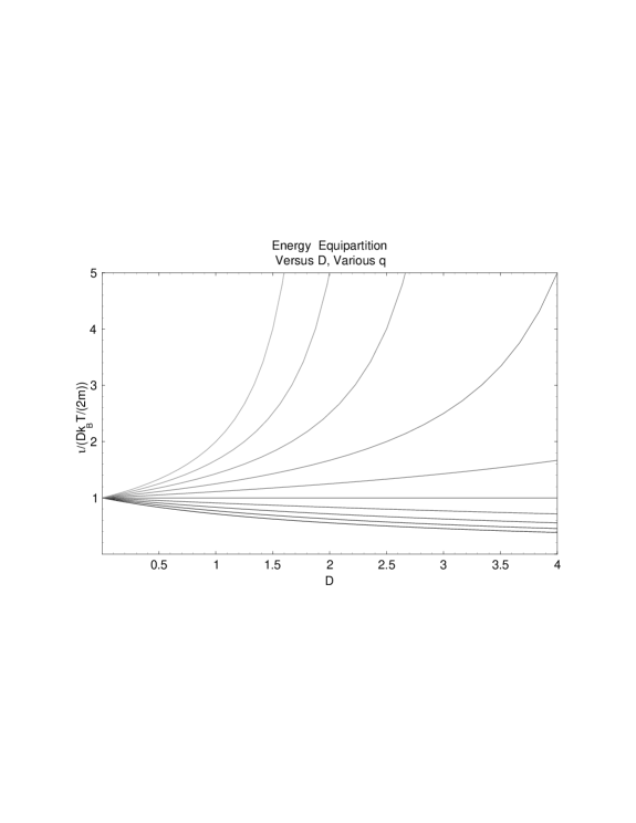
FIG. 2.: A plot of the ratio $\iota_{q}/(k_{B}T/(2m))$ versus $D$ for $q$ ranging from $0.2$ to $2.0$ in increments of $0.2$. The plot color becomes lighter as $q$ increases.

We also note from Eq. (37) that there is a hard upper bound on $q$ for this type of system. In order for the proportionality constant between $\iota_{q}$ and $T$ not to become negative, it must be that $1+(1-q)D/2>0$, or

$$q<1+\frac{2}{D}.$$ (39)

This conclusion is independent of diffeomorphic transformations in our definition of $T$ and therefore may be expected to have some general validity . A similar inequality was derived in [14]. We shall show below that hydrodynamic considerations – in particular, the positivity and finiteness of the thermal conductivity – impose an even more stringent upper bound on $q$.

Finally, the normalization constant $\Lambda$ can be expressed in terms of the mass density $\rho_{q}\equiv\frac{M_{q}}{V}$ as follows

$$\Lambda^{q}=\frac{\rho_{q}}{m}\left|\frac{m}{2\pi k_{B}T}\right|^{D/2}\left\{\begin{array}[]{ll}\frac{\left|q-1\right|^{D/2}\Gamma\left(\frac{q}{q-1}\right)}{\Gamma\left(\frac{q}{q-1}-\frac{D}{2}\right)}&\mbox{for $\sigma=+1$}\\ &\\ \frac{\left|1-q\right|^{D/2}\Gamma\left(\frac{1}{1-q}+\frac{D}{2}\right)}{\Gamma\left(\frac{1}{1-q}\right)}&\mbox{for $\sigma=-1$}\end{array}\right.$$ (40)

It follows that the global hydrodynamic equilibrium (GHE) distribution function can be written in the form

$$f^{(\mbox{eq})}({\bf z})=\left[\frac{c_{q,D}\rho_{q}}{m}\left|\frac{m}{2\pi k_{B}T}\right|^{D/2}\right]^{\frac{1}{q}}\left[1+\sigma\left|\frac{q-1}{k_{B}T}\right|\frac{m}{2}\left|{\bf v}-{\bf u}_{q}\right|^{2}\right]^{-\frac{1}{q-1}},$$ (41)

where we have defined

$$c_{q,D}\equiv\left\{\begin{array}[]{ll}\frac{\left|q-1\right|^{D/2}\Gamma\left(\frac{q}{q-1}\right)}{\Gamma\left(\frac{q}{q-1}-\frac{D}{2}\right)}&\mbox{for $\sigma=+1$}\\ &\\ \frac{\left|1-q\right|^{D/2}\Gamma\left(\frac{1}{1-q}+\frac{D}{2}\right)}{\Gamma\left(\frac{1}{1-q}\right)}&\mbox{for $\sigma=-1$,}\end{array}\right.$$ (42)

and with the proviso that $f^{(\mbox{eq})}({\bf z})=0$ if the argument raised to the $-1/(q-1)$ power in Eq. (41) is negative. This is the generalization of the Maxwell-Boltzmann distribution function for the Generalized Thermostatistics. The coefficients $c_{q,D}$ have a particularly simple form for even dimension $D$,

$$c_{q,D}=\prod_{\ell=1}^{D/2}\left[\ell-(\ell-1)q\right];$$ (43)

in particular, we note that $c_{q,2}=1$ and $c_{q,4}=2-q$. More generally, these coefficients are plotted against $q$ for various values of $D$ in Fig. 3. Various distributions for $D=1$ are illustrated in Figs. 4 and 5.

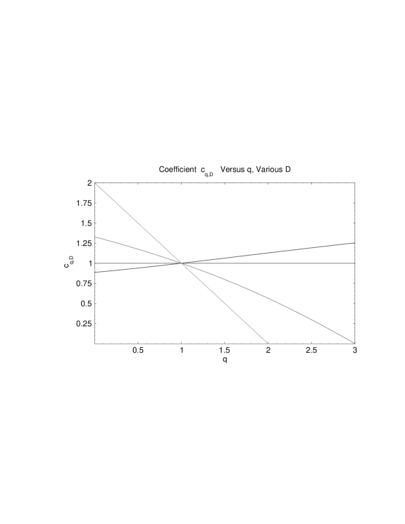
FIG. 3.: A plot of the coefficients $c_{q,D}$ versus $q$ for $D$ ranging from $1$ to $4$. The plot color becomes lighter as $D$ increases.

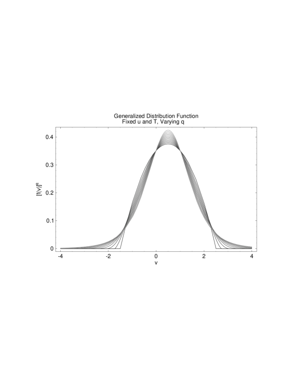
FIG. 4.: A plot of $[f^{(\mbox{eq})}({\bf z})]^{q}$ versus $v$ for $D=1$, $\rho_{q}=1$, $u_{q}=1/2$, $T=1$, and $q$ ranging from $0.5$ to $1.5$ in increments of $0.1$. The plot color becomes lighter as $q$ increases.

FIG. 5.: A plot of the equilibrium distribution function versus $v$ for $D=1$, $\rho_{q}=1$, $u_{q}=1/2$, $q=1/2$ and $T$ ranging from $0.25$ to $1.5$ in increments of $0.25$. The plot color becomes lighter as $T$ increases.

III Generalized Kinetics

A Local Hydrodynamic Equilibria

Before introducing our generalization of the BGK collision operator, we first introduce the concept of local hydrodynamic equilibrium (LHE). The GHE distribution function derived in the preceeding section is a function of velocity ${\bf v}$ alone, and independent of position ${\bf x}$. This is a direct consequence of the fact that the only conserved quantities present – mass, momentum and kinetic energy – are functions of ${\bf v}$ and not of ${\bf x}$. The GHE distribution does depend parametrically on $\rho_{q}$, ${\bf u}_{q}$ and ${\varepsilon}_{q}$, so we may write it in the more precise format $f^{(\mbox{eq})}({\bf v};\rho_{q},{\bf u}_{q},{\varepsilon}_{q})$. The LHE distribution function $f^{(0)}({\bf z})$ is then defined as having the same functional form as the GHE, but with parameters $\rho_{q}$, ${\bf u}_{q}$ and ${\varepsilon}_{q}$ weakly dependent on spatial position ${\bf x}$. That is,

$$f^{(0)}({\bf z})=f^{(\mbox{eq})}({\bf v};\rho_{q}({\bf x}),{\bf u}_{q}({\bf x}),{\varepsilon}_{q}({\bf x})).$$ (44)

It should be noted that the LHE, unlike the GHE, is not expected to be a stationary state of the system. If the system is initialized in a LHE distribution, its time evolution will generally take it away from this simple functional form. That is, the full solution to the system’s kinetic equation should be expected to be the LHE plus a correction. To the extent that the spatial gradients are weak, this correction will be small and can be treated perturbatively. This is the basis of the Chapman-Enskog expansion.

B The Generalized BGK Equation and $H$-Theorem

Armed with the concept of LHE, we propose the following generalization of the Boltzmann equation with the BGK collision operator:

$$\left(\frac{\partial}{\partial t}+{\bf v}\cdot{\mbox{\boldmath$\nabla$}}\right)\left[f({\bf z})\right]^{q}=-\frac{1}{\tau}\left\{\left[f({\bf z})\right]^{q}-\left[f^{(0)}({\bf z})\right]^{q}\right\},$$ (45)

where $f^{(0)}({\bf z})$ is the LHE distribution function that is defined as having the same moments as the exact distribution function $f({\bf z})$,

$$\left(\begin{array}[]{c}\rho_{q}\\ \rho_{q}{\bf u}_{q}\\ \rho_{q}{\varepsilon}_{q}\end{array}\right)=\int d{\bf v}\;\left[f({\bf z})\right]^{q}\left(\begin{array}[]{c}m\\ m{\bf v}\\ mv^{2}/2\end{array}\right)=\int d{\bf v}\;\left[f^{(0)}({\bf z})\right]^{q}\left(\begin{array}[]{c}m\\ m{\bf v}\\ mv^{2}/2\end{array}\right),$$ (46)

and where $\tau>0$ is the collisional relaxation time. In spite of the deceptively simple appearance of Eq. (45), note that it is nonlinear even when $q=1$. This is because of Eq. (46) which requires that the moments of $f^{(0)}({\bf z})$, which determine the parameters that appear nonlinearly in its functional form, are themselves functionals of $f({\bf z})$. To see this more clearly, note that Eqs. (44) and (46) can be used to rewrite Eq. (45) in the explicitly nonlinear but woefully cumbersome form

$$\left(\frac{\partial}{\partial t}+{\bf v}\cdot{\mbox{\boldmath$\nabla$}}\right)\left[f({\bf z})\right]^{q}=-\frac{1}{\tau}\left\{\left[f({\bf z})\right]^{q}-\left[f^{(\mbox{eq})}\left({\bf v};\int d{\bf v}\;[f({\bf z})]^{q}m,\int d{\bf v}\;[f({\bf z})]^{q}m{\bf v},\int d{\bf v}\;[f({\bf z})]^{q}\frac{m}{2}v^{2}\right)\right]^{q}\right\}.$$ (47)

Hence, when $q\neq 1$, this departs from the usual BGK equation in two important respects: First, and most obviously, it is constructed so that it relaxes to the explicitly $q$-dependent LHE $f^{(0)}({\bf z})$, given by Eqs. (44) and (41), rather than to the usual Maxwell-Boltzmann LHE. Second, the nonlinearity in the collision operator arises via the functional form of $[f^{(0)}]^{q}$ which also explicitly depends on $q$. It is important to keep these two mechanisms clearly in mind because a superficial glance at Eq. (45) might suggest that the substitution $F({\bf z})\equiv[f({\bf z})]^{q}$ will render its dynamics identical to those of the usual BGK equation, and this is not so.

Eq. (45) is a sensible generalization of the BGK equation for three reasons. First, it obviously reduces to the usual BGK equation when $q=1$. Second, if we multiply it by the $\gamma^{i}({\bf z})$ and integrate over ${\bf v}$, we find local conservation equations

$$0=\frac{\partial}{\partial t}\left(\begin{array}[]{c}\rho_{q}({\bf x})\\ {\bf p}_{q}({\bf x})\\ {\varepsilon}_{q}({\bf x})\end{array}\right)+{\mbox{\boldmath$\nabla$}}\cdot\int d{\bf v}\;\left[f(z)\right]^{q}\left(\begin{array}[]{c}m{\bf v}\\ m{\bf v}{\bf v}\\ m{\bf v}v^{2}/2\end{array}\right)$$ (48)

for each of the conserved quantities. Third, we can show that Eq. (45) obeys an $H$-theorem – at least for $q>0$ – as follows:

$$\frac{d}{dt}S_{q}[f] = \int d{\bf z}\;\left\{\frac{\delta S_{q}[f]}{\delta f(z)}\right\}\frac{\partial f({\bf z})}{\partial t}$$ (49)

$$= \frac{k_{B}}{q-1}\int d{\bf z}\;\left\{1-q[f({\bf z})]^{q-1}\right\}\frac{\partial f({\bf z})}{\partial t}$$ (50)

$$= \frac{k_{B}}{q-1}\int d{\bf z}\;\left\{\frac{1}{q[f({\bf z})]^{q-1}}-1\right\}\frac{\partial}{\partial t}[f({\bf z})]^{q}$$ (51)

$$= \frac{k_{B}}{q-1}\int d{\bf z}\;\left\{\frac{1}{q[f({\bf z})]^{q-1}}-1\right\}\left(\frac{\partial}{\partial t}+{\bf v}\cdot{\mbox{\boldmath$\nabla$}}\right)[f({\bf z})]^{q}$$ (52)

$$= -\frac{k_{B}}{(q-1)\tau}\int d{\bf z}\;\left\{\frac{1}{q[f({\bf z})]^{q-1}}-1\right\}\left\{[f({\bf z})]^{q}-[f^{(0)}({\bf z})]^{q}\right\}$$ (53)

$$= \frac{S_{q}\left[f^{(0)}\right]-S_{q}\left[f\right]}{\tau}+\frac{k_{B}}{(q-1)\tau}\int d{\bf z}\;\left\{\left[f({\bf z})-f^{(0)}({\bf z})\right]-\frac{[f({\bf z})]^{q}-[f^{(0)}({\bf z})]^{q}}{q[f({\bf z})]^{q-1}}\right\}$$ (54)

$$= \frac{S_{q}\left[f^{(0)}\right]-S_{q}\left[f\right]}{\tau}+\frac{k_{B}}{(q-1)\tau}\int d{\bf z}\;f^{(0)}({\bf z})\left\{\left[g({\bf z})-1\right]-\frac{[g({\bf z})]^{q}-1}{q[g({\bf z})]^{q-1}}\right\}$$ (55)

$$= \frac{S_{q}\left[f^{(0)}\right]-S_{q}\left[f\right]}{\tau}+\frac{k_{B}}{\tau}\int d{\bf z}\;f^{(0)}({\bf z})\Phi_{q}\left(g({\bf z})\right),$$ (56)

where $g({\bf z})\equiv f({\bf z})/f^{(0)}({\bf z})>0$, the domain has been assumed to be without boundary, and where we have defined the function

$$\Phi_{q}(x)\equiv\frac{1}{q-1}\left[\left(x-1\right)-\frac{x^{q}-1}{qx^{q-1}}\right].$$ (57)

The first term of Eq. (56) is nonnegative since the entropy is a maximum for the distribution function $f^{(0)}({\bf z})$ and $q>0$ by construction. It is not difficult to show that the function $\Phi_{q}$ is nonnegative for positive argument (see Fig. 6), so the second term is also nonnegative. It follows that $dS_{q}[f]/dt\geq 0$ for $q>0$, with equality holding only at equilibrium.

FIG. 6.: A plot of the function $\Phi_{q}(x)$ versus $x$ for $q\in\{0.25,0.50,0.75,1.00,1.25,1.50\}$. The plot color becomes lighter as $q$ increases.

For $q<0$, the generalized entropy $S_{q}[f]$ is minimized at its extremum, rather than maximized, as can be seen from examination of its second variation. In this situation, the first term on the right-hand side of Eq. (56) is negative, but the second term is still positive because $\Phi_{q}(x)\geq 0$ still holds for $q\leq 0$. Hence the above argument breaks down and a more subtle one is needed. We shall not concern ourselves with the case $q\leq 0$ in this paper.

IV The Chapman-Enskog Analysis

A The Asymptotic Expansion

We now develop the distribution function in a perturbation series where the zero-order approximation is the LHE, following the program described in Subsection III A. We rewrite our generalized BGK equation, Eq. (45), in the form

$$\left(1+\tau{\hat{\cal D}}\right)F({\bf z})=F^{(\mbox{$0$})}({\bf z}),$$ (58)

where we have defined

$$F({\bf z}) \equiv \left[f({\bf z})\right]^{q}$$ (59)

$$F^{(\mbox{$0$})}({\bf z}) \equiv \left[f^{(\mbox{$0$})}({\bf z})\right]^{q},$$ (61)

and the operator

$${\hat{\cal D}}\equiv\frac{\partial}{\partial t}+{\bf v}\cdot{\mbox{\boldmath$\nabla$}}.$$ (62)

The formal solution to the above equation is

$$F({\bf z})=\left(1+\tau{\hat{\cal D}}\right)^{-1}F^{(\mbox{$0$})}({\bf z}).$$ (63)

Following the standard Chapman-Enskog procedure [15], we expand the derivative in a series of successively more slowly varying time scales,

$${\hat{\cal D}}=\sum_{j=1}^{\infty}\epsilon^{j}{\hat{\cal D}}_{j},$$ (64)

where

$${\hat{\cal D}}_{j}\equiv\frac{\partial}{\partial t_{j}}+{\bf v}\cdot{\mbox{\boldmath$\nabla$}},$$ (65)

where $\epsilon$ is a formal expansion parameter, and $t_{j}$ is the $j$th time scale. To second order in $\epsilon$, we find

$$F({\bf z})=\left[1-\epsilon\tau{\hat{\cal D}}_{1}-\epsilon^{2}\tau\left({\hat{\cal D}}_{2}-\tau{\hat{\cal D}}_{1}^{2}\right)+\cdots\right]F^{(\mbox{$0$})}({\bf z}).$$ (66)

Thus we have

$$F({\bf z})=\sum_{n=0}^{\infty}\epsilon^{n}F^{(\mbox{$n$})}({\bf z}),$$ (67)

where

$$F^{(\mbox{$1$})}({\bf z}) = -\tau{\hat{\cal D}}_{1}F^{(\mbox{$0$})}({\bf z})$$ (68)

$$F^{(\mbox{$2$})}({\bf z}) = -\tau\left({\hat{\cal D}}_{2}-\tau{\hat{\cal D}}_{1}^{2}\right)F^{(\mbox{$0$})}({\bf z}).$$ (69)

$$\vdots$$ (70)

The higher order terms $F^{(\mbox{$1$})}$ and $F^{(\mbox{$2$})}$ must not change the definition of the conserved densities,

$$0=\int d{\bf v}\;\left[F({\bf z})-F^{(\mbox{$0$})}({\bf z})\right]\left(\begin{array}[]{c}m{\bf v}\\ m{\bf v}{\bf v}\\ m{\bf v}v^{2}/2\end{array}\right)=\sum_{n=1}^{\infty}\epsilon^{n}\int d{\bf v}\;F^{(\mbox{$n$})}({\bf z})\left(\begin{array}[]{c}m{\bf v}\\ m{\bf v}{\bf v}\\ m{\bf v}v^{2}/2\end{array}\right).$$ (71)

To fully specify the determination of the $F^{(\mbox{$n$})}$, we further require that they satisfy Eq. (71) order by order; that is,

$$0=\int d{\bf v}\;F^{(\mbox{$n$})}({\bf z})\left(\begin{array}[]{c}m{\bf v}\\ m{\bf v}{\bf v}\\ m{\bf v}v^{2}/2\end{array}\right)$$ (72)

for $n\geq 1$.

B The First-Order Solution

At first order, Eq. (68) can be written

$$F^{(\mbox{$1$})}({\bf z})=-\tau\left(\frac{\partial}{\partial t_{1}}+{\bf v}\cdot{\mbox{\boldmath$\nabla$}}\right)F^{(\mbox{$0$})}({\bf z}).$$ (73)

We take the hydrodynamic moments of both sides, noting that the left-hand side will vanish thanks to Eq. (72). We get

$$0=\frac{\partial}{\partial t_{1}}\left(\begin{array}[]{c}\rho_{q}\\ \rho_{q}{\bf u}_{q}\\ \rho_{q}{\varepsilon}_{q}\end{array}\right)+{\mbox{\boldmath$\nabla$}}\cdot\int d{\bf v}\;F^{(\mbox{$0$})}({\bf z})\left(\begin{array}[]{c}m{\bf v}\\ m{\bf v}{\bf v}\\ m{\bf v}v^{2}/2\end{array}\right).$$ (74)

The first of these is immediately seen to be the usual equation expressing conservation of mass

$$0=\frac{\partial\rho_{q}}{\partial t_{1}}+{\mbox{\boldmath$\nabla$}}\cdot\left(\rho_{q}{\bf u}_{q}\right),$$ (75)

which is thus seen to be $q$-invariant at first order.

To evaluate the momentum equation at first order, we must integrate the dyad $m{\bf v}{\bf v}$ times $F^{(\mbox{$0$})}$. We have

$$\int d{\bf v}\;F^{(\mbox{$0$})}({\bf z})m{\bf v}{\bf v} = \int d{\bf v}\;F^{(\mbox{$0$})}({\bf z})m\left[\left({\bf v}-{\bf u}_{q}\right)+{\bf u}_{q}\right]\left[\left({\bf v}-{\bf u}_{q}\right)+{\bf u}_{q}\right]$$ (76)

$$= \rho_{q}{\bf u}_{q}{\bf u}_{q}+\left(\frac{2k_{B}}{m}\left|\frac{T}{q-1}\right|\right)^{\frac{D}{2}+1}\int d{\bf w}\;F^{(\mbox{$0$})}({\bf z})m{\bf w}{\bf w},$$ (77)

since the odd cross terms integrate to zero. Turning our attention to the last integral over ${\bf w}$, it is clear from parity that only the diagonal elements of this dyad will have nonvanishing integral, and from isotropy that they will all give the same result. Thus, we have

$$\int d{\bf v}\;F^{(\mbox{$0$})}({\bf z})m{\bf v}{\bf v}=\rho_{q}{\bf u}_{q}{\bf u}_{q}+{\bf 1}\left(\frac{2k_{B}}{m}\left|\frac{T}{q-1}\right|\right)^{\frac{D}{2}+1}\int d{\bf w}\;F^{(\mbox{$0$})}({\bf z})mw_{x}^{2}.$$ (78)

To perform this last integral, the spherically symmetric volume element of Eq. (20) is inadequate. Rather, we write $w_{x}=w\cos\theta$, where $0\leq\theta\leq\pi$ is a polar angle, and we adopt the cylindrically symmetric volume element

$$d{\bf w}=\frac{2\pi^{\frac{D-1}{2}}}{\Gamma\left(\frac{D-1}{2}\right)}w^{D-1}dw\;d\theta.$$ (79)

Now both the $w$ and $\theta$ integrals yield beta-functions which must be considered for both cases $\sigma=\pm 1$. The result, which does not depend on $\sigma$, is then

$$\int d{\bf v}\;F^{(\mbox{$0$})}({\bf z})m{\bf v}{\bf v}=\rho_{q}{\bf u}_{q}{\bf u}_{q}+P_{q}{\bf 1}$$ (80)

where we have defined the pressure

$$P_{q}\equiv\frac{\rho_{q}k_{B}T}{m\left[1+(1-q)\frac{D}{2}\right]}.$$ (81)

The momentum equation at first order is thus

$$0=\frac{\partial}{\partial t_{1}}\left(\rho_{q}{\bf u}_{q}\right)+{\mbox{\boldmath$\nabla$}}\cdot\left(\rho_{q}{\bf u}_{q}{\bf u}_{q}+P_{q}{\bf 1}\right).$$ (82)

Eq. (81) appears to be a nonideal equation of state for the pressure but, as noted at the end of the previous subsection, we must avoid attaching physical significance to the temperature $T$. Rather, we should take care to relate observable quantities – in this case, the pressure $P_{q}$ and the internal energy $\iota_{q}$. From Eqs. (81) and (37), we have

$$P_{q}=\frac{2}{D}\rho_{q}\iota_{q},$$ (83)

and this is the usual ideal gas equation of state with no correction, which we see is $q$-invariant after all.

Finally, we consider the energy equation at first order. We must integrate the vector $m{\bf v}v^{2}/2$ times $F^{(\mbox{$0$})}$. We have

$$\int d{\bf v}\;F^{(\mbox{$0$})}({\bf z})\frac{m{\bf v}v^{2}}{2} = \int d{\bf v}\;F^{(\mbox{$0$})}({\bf z})\frac{m}{2}\left[\left({\bf v}-{\bf u}_{q}\right)+{\bf u}_{q}\right]\left|\left({\bf v}-{\bf u}_{q}\right)+{\bf u}_{q}\right|^{2}$$ (84)

$$= \rho_{q}{\varepsilon}_{q}{\bf u}_{q}+{\bf u}_{q}\cdot\left[\left(\frac{2k_{B}}{m}\left|\frac{T}{q-1}\right|\right)^{\frac{D}{2}+1}\int d{\bf w}\;F^{(\mbox{$0$})}({\bf z})m{\bf w}{\bf w}\right]$$ (85)

since the odd cross terms integrate to zero. The quantity in square brackets in the second term is the same one we encountered in the definition of the pressure and is equal to $P_{q}{\bf 1}$. The energy equation at first order is thus

$$0=\frac{\partial}{\partial t_{1}}\left(\rho_{q}{\varepsilon}_{q}\right)+{\mbox{\boldmath$\nabla$}}\cdot\left[\left(\rho_{q}{\varepsilon}_{q}+P_{q}\right){\bf u}_{q}\right].$$ (86)

Eqs. (75), (82) and (86) give us the rate of change of the hydrodynamic variables on time scale $t_{1}$. They and the equation of state, Eq. (83), are all seen to be $q$-invariant. Thus, at first order, there is no experiment that we could perform that would distinguish a system with $q\neq 1$ from the more orthodox $q=1$ case. To make this distinction, we must examine the dissipative terms that appear at second order in the Chapman-Enskog analysis, and we turn our attention to those now.

C The Second-Order Solution

At second order, Eq. (69) can be written

$$F^{(\mbox{$2$})}({\bf z})=-\tau\left[\left(\frac{\partial}{\partial t_{2}}+{\bf v}\cdot{\mbox{\boldmath$\nabla$}}\right)F^{(\mbox{$0$})}({\bf z})-\tau\left(\frac{\partial}{\partial t_{1}}+{\bf v}\cdot{\mbox{\boldmath$\nabla$}}\right)^{2}F^{(\mbox{$0$})}({\bf z})\right].$$ (87)

Again, we take the hydrodynamic moments of both sides, noting that the left-hand side will vanish thanks to Eq. (72). Drawing on our experience from the first-order calculation, we see that we get

$$\frac{\partial}{\partial t_{2}}\left(\begin{array}[]{c}\rho_{q}\\ \rho_{q}{\bf u}_{q}\\ \rho_{q}{\varepsilon}_{q}\end{array}\right)+{\mbox{\boldmath$\nabla$}}\cdot\left(\begin{array}[]{c}\rho_{q}{\bf u}_{q}\\ \rho_{q}{\bf u}_{q}{\bf u}_{q}+P_{q}{\bf 1}\\ \left(\rho_{q}{\varepsilon}_{q}+P_{q}\right){\bf u}_{q}\end{array}\right)$$ (94)

$$= \tau\left[\frac{\partial^{2}}{\partial t_{1}^{2}}\left(\begin{array}[]{c}\rho_{q}\\ \rho_{q}{\bf u}_{q}\\ \rho_{q}{\varepsilon}_{q}\end{array}\right)+2\frac{\partial}{\partial t_{1}}{\mbox{\boldmath$\nabla$}}\cdot\left(\begin{array}[]{c}\rho_{q}{\bf u}_{q}\\ \rho_{q}{\bf u}_{q}{\bf u}_{q}+P_{q}{\bf 1}\\ \left(\rho_{q}{\varepsilon}_{q}+P_{q}\right){\bf u}_{q}\end{array}\right)+{\mbox{\boldmath$\nabla$}}{\mbox{\boldmath$\nabla$}}:\int d{\bf v}\;{\bf v}{\bf v}F^{(\mbox{$0$})}({\bf z})\left(\begin{array}[]{c}m\\ m{\bf v}\\ mv^{2}/2\end{array}\right)\right]$$ (104)

$$= \tau{\mbox{\boldmath$\nabla$}}\cdot\left[\frac{\partial}{\partial t_{1}}\left(\begin{array}[]{c}\rho_{q}{\bf u}_{q}\\ \rho_{q}{\bf u}_{q}{\bf u}_{q}+P_{q}{\bf 1}\\ \left(\rho_{q}{\varepsilon}_{q}+P_{q}\right){\bf u}_{q}\end{array}\right)+{\mbox{\boldmath$\nabla$}}\cdot\int d{\bf v}\;{\bf v}{\bf v}F^{(\mbox{$0$})}({\bf z})\left(\begin{array}[]{c}m\\ m{\bf v}\\ mv^{2}/2\end{array}\right)\right],$$ (111)

where we used the first order results in the second step. Note that the right-hand side is now manifestly a divergence. The quantity inside this divergence is the negative of a diffusive flux. The derivatives with respect to $t_{1}$ can be eliminated using the first-order evolution equations.

The right-hand side of the second-order mass conservation equation is seen to vanish due to the first-order momentum conservation equation. Thus, we find that the form of the mass conservation equation

$$0=\frac{\partial\rho_{q}}{\partial t_{2}}+{\mbox{\boldmath$\nabla$}}\cdot\left(\rho_{q}{\bf u}_{q}\right)$$ (112)

is $q$-invariant to second order.

To evaluate the right-hand side of the momentum equation at second order, we must integrate the triad $m{\bf v}{\bf v}{\bf v}$ times $F^{(\mbox{$0$})}$. The procedure is the same as that at first order, and no new moments need to be defined. The result in index notation is

$$\int d{\bf v}\;F^{(\mbox{$0$})}({\bf z})mv_{i}v_{j}v_{k}=\rho_{q}{u_{q}}_{i}{u_{q}}_{j}{u_{q}}_{k}+P_{q}\left(\delta_{ij}{u_{q}}_{k}+\delta_{ik}{u_{q}}_{j}+\delta_{jk}{u_{q}}_{i}\right).$$ (113)

Inserting this into the second-order momentum equation, carrying out the derivatives with respect to $t_{1}$ using the first-order equations, and simplifying, we get

$$\frac{\partial}{\partial t_{2}}\left(\rho_{q}{\bf u}_{q}\right)+{\mbox{\boldmath$\nabla$}}\cdot\left(\rho_{q}{\bf u}_{q}{\bf u}_{q}+P_{q}{\bf 1}\right)={\mbox{\boldmath$\nabla$}}\cdot\left\{\mu_{q}\left[{\mbox{\boldmath$\nabla$}}{\bf u}_{q}+\left({\mbox{\boldmath$\nabla$}}{\bf u}_{q}\right)^{T}\right]+\lambda_{q}\left({\mbox{\boldmath$\nabla$}}\cdot{\bf u}_{q}\right){\bf 1}\right\},$$ (114)

where the superscript $T$ denotes “transpose,” and where we have defined the shear viscosity

$$\mu_{q}\equiv\frac{2\tau}{D}\rho_{q}\iota_{q},$$ (115)

and the bulk viscosity

$$\lambda_{q}\equiv-\frac{4\tau}{D^{2}}\rho_{q}\iota_{q}.$$ (116)

Here we have used the equation of state, Eq. (83), to express the viscosities in terms of the internal energy. Note that Eqs. (115) and (116) are $q$-invariant, as is the ratio

$$\frac{\lambda_{q}}{\mu_{q}}=-\frac{2}{D}$$ (117)

which is known to be approximately true for a variety of real gases [19]. Thus, measurement of the ratio of the viscosities is still insufficient to determine $q$ experimentally.

Finally, we turn our attention to the energy equation at second order. For this we must integrate the diad $m{\bf v}{\bf v}v^{2}/2$ times $F^{(\mbox{$0$})}$. The by now familiar procedure again yields beta-function integrals which must be considered for both cases $\sigma=\pm 1$. The result, which does not depend on $\sigma$, is then

$$\int d{\bf v}\;F^{(\mbox{$0$})}({\bf z})m{\bf v}{\bf v}\frac{v^{2}}{2}=\left(\rho_{q}{\varepsilon}_{q}+2P_{q}\right){\bf u}_{q}{\bf u}_{q}+\left\{P_{q}\frac{u_{q}^{2}}{2}+\frac{4}{D^{2}}\left(\frac{D}{2}+1\right)\left[\frac{1+(1-q)\frac{D}{2}}{1+(1-q)\left(\frac{D}{2}+1\right)}\right]\rho_{q}\iota_{q}^{2}\right\}{\bf 1}.$$ (118)

Inserting this into the second-order energy equation, carrying out the derivatives with respect to $t_{1}$ using the first-order equations, and simplifying, we get

$$\frac{\partial}{\partial t_{2}}\left(\rho_{q}{\varepsilon}_{q}\right)+{\mbox{\boldmath$\nabla$}}\cdot\left[\left(\rho_{q}{\varepsilon}_{q}+P_{q}\right){\bf u}_{q}\right]$$ (119)

$$= {\mbox{\boldmath$\nabla$}}\cdot\left\{{\bf u}_{q}\cdot\left[\mu_{q}\left({\mbox{\boldmath$\nabla$}}{\bf u}_{q}+\left({\mbox{\boldmath$\nabla$}}{\bf u}_{q}\right)^{T}\right)+\lambda_{q}\left({\mbox{\boldmath$\nabla$}}\cdot{\bf u}_{q}\right){\bf 1}\right]+k_{q}{\mbox{\boldmath$\nabla$}}\iota_{q}-(1-q)\frac{a_{q}}{\rho_{q}}{\mbox{\boldmath$\nabla$}}\left(\rho_{q}\iota_{q}\right)\right\}$$ (120)

where we have defined the thermal conductivity

$$k_{q}\equiv\frac{4}{D^{2}}\left(1+\frac{D}{2}\right)\left[\frac{1+(1-q)\frac{D}{2}}{1+(1-q)\left(\frac{D}{2}+1\right)}\right]\tau\rho_{q}\iota_{q},$$ (121)

and the anomalous transport coefficient

$$a_{q}\equiv\frac{4}{D^{2}}\left[\frac{\frac{D}{2}+1}{1+(1-q)\left(\frac{D}{2}+1\right)}\right]\tau\rho_{q}\iota_{q}.$$ (122)

We note that positivity and finiteness of the thermal conductivity sets an even more stringent upper bound on $q$ than Eq. (39), namely

$$q<1+\frac{2}{D+2}.$$ (123)

We emphasize that this inequality is not expected to hold for general systems; its derivation was specific to our assumption of an ideal gas.

The most striking feature of the second-order energy conservation equation, Eq. (120), is that it is not $q$-invariant. Its diffusive flux contains a term proportional to $(1-q){\mbox{\boldmath$\nabla$}}\left(\rho_{q}\iota_{q}\right)/\rho_{q}$ with a new transport coefficient $a_{q}$. The presence of this term can be detected by purely hydrodynamic experiments and this may be used to test whether or not $q$ is equal to unity. Moreover, we see that the ratio

$$\frac{a_{q}}{k_{q}}=\left[1+(1-q)\frac{D}{2}\right]^{-1}$$ (124)

gives us another means of determining $q$, as does the ratio

$$\frac{k_{q}}{\mu_{q}}=\frac{2}{D}\left(\frac{D}{2}+1\right)\left[\frac{1+(1-q)\frac{D}{2}}{1+(1-q)\left(\frac{D}{2}+1\right)}\right].$$ (125)

These ratios are plotted in Figs. 7 and 8.

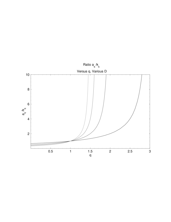
FIG. 7.: A plot of the ratio of the anomalous transport coefficient $a_{q}$ to the thermal conductivity $k_{q}$ for $D$ ranging from $1$ to $4$. The plot color becomes lighter as $D$ increases.

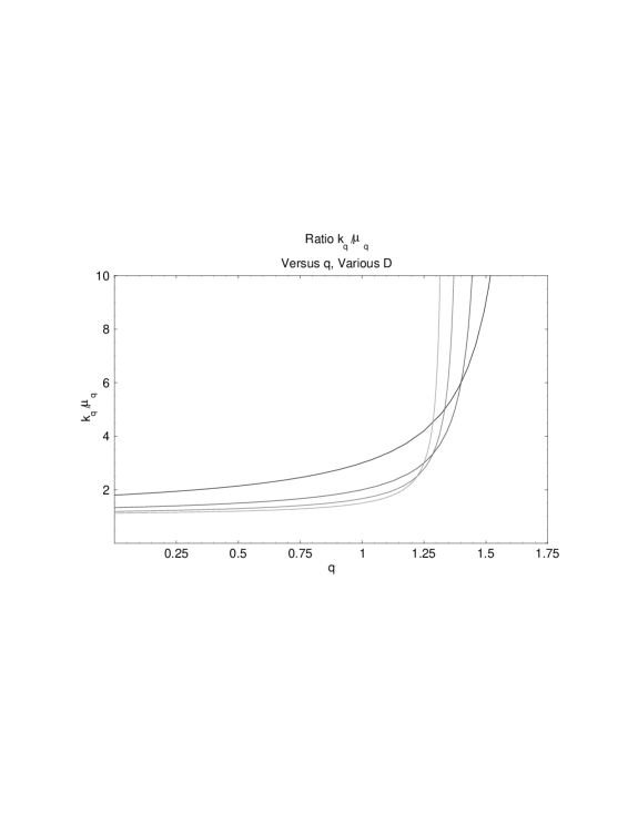
FIG. 8.: A plot of the ratio of the thermal conductivity $k_{q}$ to the shear viscosity $\mu_{q}$ for $D$ ranging from $1$ to $4$. The plot color becomes lighter as $D$ increases.

V Discussion

Eqs. (112), (114) and (120) constitute the compressible Navier-Stokes equations for the generalized thermostatistics. We see that the mass and momentum conservation equations are completely $q$-invariant, but the energy conservation equation is not. It contains a term that is proportional to $(1-q){\mbox{\boldmath$\nabla$}}\left(\rho_{q}\iota_{q}\right)/\rho_{q}$ which vanishes for Boltzmann-Gibbs statistics. It is a term not normally included in presentations of the Navier-Stokes equations.

In addition, we have shown that certain ratios of the transport coefficients may be $q$ dependent. While the famous result $\lambda_{q}/\mu_{q}=-2/D$ appears to be $q$-invariant, the ratios $k_{q}/\mu_{q}$ and $a_{q}/k_{q}$ are decidedly less robust and may be used to infer a value of $q$. At this point, the reader may be tempted to pick up a handbook of material properties, search for materials with anomalous ratios of thermal conductivity to shear viscosity, and attribute those anomalies to a breakdown in Boltzmann-Gibbs statistics for those materials. The reader is implored to resist this temptation. There are very many potential pitfalls in the Boltzmann/Chapman-Enskog analysis that are far more likely to generate such anomalies than a breakdown in the foundations of thermostatistics. The presence of rotational and/or internal molecular degrees of freedom, high densities leading to three-body collisions, and violations of the Boltzmann molecular chaos assumption are but three examples of phenomena that might also cause such anomalies. If, however, one has other reasons to believe that a particular system violates Boltzmann-Gibbs thermostatistics, then examination of the ratios of the transport coefficients may provide further corroboration. One does have such reason to believe this for the stellar polytrope and pure-electron plasma examples mentioned earlier; unfortunately, those systems of particles are not ideal gases in any reasonable sense of the term so, even if one could measure the transport coefficients of such things, the quantitative results derived above should not be expected to apply.

In summary, the presence of the anomalous term in the energy equation of a dilute gas would seem to be the easiest way to search for deviations of $q$ from unity. I am currently unaware of any experimental work that would clearly establish either the presence or absence of this term. I leave it to my colleagues who have more familiarity with the experimental hydrodynamic literature to sort out this matter.

VI Conclusions

We have shown that the Navier-Stokes equations for mass and momentum conservation are $q$-invariant to second order in the Chapman-Enskog expansion, but that the equation for energy conservation is not. We have derived the form of this anomalous term, using a generalized Chapman-Enskog analysis on a generalized BGK kinetic equation. In addition, we have found $q$-dependent anomalies in ratios of certain transport coefficients – in particular, in the ratio of the thermal conductivity to the shear viscosity. Finally, we have found that hydrodynamics gives rise to the upper bound $q<1+2/(D+2)$ which is more stringent than that imposed by equilibrium considerations.

This work could be substantially improved by using a more realistic kinetic equation, but we have argued that the principal results – the form of the hydrodynamic equations, and the ratios of the transport coefficients – ought to be robust in this regard. It is hoped that some of the insights obtained in this analysis will eventually be useful in constructing simple experimental tests for the presence of breakdowns in Boltzmann-Gibbs statistics.

REFERENCES

- [1] C. Tsallis, J. Stat. Phys. 52 (1988) 479; Physica A 221 (1995) 277.
- [2] E.M.F. Curado, C. Tsallis, J. Phys. A: Math. Gen. 24 L69.
- [3] A. Chame, E.V.L. de Mello, Phys. Lett. A 228 (1997) 159.
- [4] A. Chame, E.V.L. de Mello, J. Phys. A 27 (1994) 3663.
- [5] A.R. Plastino, A. Plastino, Phys. Lett. A 174 (1993) 384-386.
- [6] B.M. Boghosian, Phys. Rev. E 53 (1996) 4754-4763.
- [7] C. Anteneodo, C. Tsallis, J. Mol. Liq. 71 (1997) 255-267.
- [8] P.A. Alemany, D.H. Zanette, Phys. Rev. E 49 (1994) R956.
- [9] C. Tsallis, S.V.F. Levy, A.M.C. de Souza, R. Maynard, Phys. Rev. Lett. 75 (1995) 3589; Erratum: Phys. Rev. Lett. 77 (1996) 5442.
- [10] C. Tsallis, Physics World (July, 1997) 42.
- [11] C. Tsallis, A.M.C. de Souza, Phys. Lett. A 235 (1997) 444-446.
- [12] N. Goldenfeld, “Lectures on Phase Transitions and the Renormalization Group,” Addison-Wesley (1992) 27-28.
- [13] M. Abramowitz and I.A. Stegun, “Handbook of Mathematical Functions,” National Bureau of Standards (ninth printing, 1970) p. 258.
- [14] A.R. Plastino, A. Plastino, C. Tsallis, J. Phys. A: Math. Gen. 27 (1994) 5707-5714.
- [15] K. Huang, “Statistical Physics,” John Wiley and Sons (third printing, 1966).
- [16] C. Tsallis, R.S. Mendes, A.R. Plastino, Physica A 261 (1998) 534.
- [17] S. Abe, “Thermodynamic Limit and Classical Ideal Gas in Nonextensive Statistical Mechanics with Normalised -Expectation Values,” preprint (1998).
- [18] C. Anteneodo, private communication (1998).
- [19] F.H. Harlow, A.A. Amsden, “Fluid Dynamics – A LASL Monograph,” Los Alamos publication LA-4700 (1971).