Ferromagnetism and the temperature-dependent electronic structure in thin Hubbard films

Abstract

The magnetic behavior of thin ferromagnetic itinerant-electron films is investigated within the strongly correlated single-band Hubbard model. For its approximate solution we apply a generalization of the modified alloy analogy (MAA) to deal with the modifications due to the reduced translational symmetry. The theory is based on exact results in the limit of strong Coulomb interaction which are important for a reliable description of ferromagnetism. Within the MAA the actual type of the alloy analogy is determined selfconsistently. The MAA allows, in particular, the investigation of quasiparticle lifetime effects in the paramagnetic as well as the ferromagnetic phase. For thin fcc(100) and fcc(111) films the layer magnetizations are discussed as a function of temperature as well as film thickness. The magnetization at the surface-layer is found to be reduced compared to the inner layers. This reduction is stronger in fcc(100) than in fcc(111) films. The magnetic behavior can be microscopically understood by means of the layer-dependent spectral density and the quasiparticle density of states. The quasiparticle lifetime that corresponds to the width of the quasiparticle peaks in the spectral density is found to be strongly spin- and temperature-dependent.

1 Introduction

Remarkable advances in thin film technology have recently led to active interest in the nature of magnetism in ultrathin films, at surfaces and multilayer structures. The influence of the reduced dimensionality on the magnetic behavior of $3d$ transition metals has been extensively studied both experimentally [1, 2, 3, 4, 5, 6, 7] and theoretically [8, 9, 10, 11, 12, 13, 14, 15, 16]. On the experimental side it was shown that ultrathin transition metal films can display long range ferromagnetic order from a monolayer on [5]. Although the Mermin-Wagner theorem [17] requires the transition temperature to vanish for perfectly isotropic two dimensional systems, it was shown theoretically that even a small amount of anisotropy may lead to magnetic order with a substantial transition temperature [18, 19, 20]. In real materials magnetic anisotropy is always present by virtue of either the dipole interaction or the spin-orbit coupling.

Theoretically, the $T=0\,$K properties of thin transition metal films have been addressed by ab initio calculations within the density functional theory in the local density approximation [8, 9, 10, 11]. However, these approaches are strictly based on a Stoner-type model of ferromagnetism and, therefore, treat electron correlation effects which are responsible for the spontaneous magnetic order on a low level. In addition they are restricted to ground state properties only. To overcome this restriction, for example, a generalization of the fluctuating local moment method has been used [13] to calculate the temperature-dependent electronic structure of thin ferromagnetic films. However, the layer magnetizations at finite temperatures and the magnetic short range order are needed as an input. In Ref. [12] magnetic phase transitions in thin films are investigated via a mapping of the ab initio results onto an effective Ising model. Hasegawa calculates the finite temperature properties of thin Cu/Ni/Cu sandwiches by use of the single-site spin-fluctuation theory [21].

For the understanding of the thermodynamical properties of thin film magnetism theoretical investigations on rather idealized model systems have proven to be a good starting point. In this context several authors have focused on localized spin models like the Heisenberg model [22, 23, 24, 25]. For example, the mechanism that leads to the experimentally observed temperature induced reorientation of the direction of magnetization in thin Fe and Ni films [6, 7] was investigated in great detail [26, 27]. On the other hand it is by no means clear to what extent the results obtained by localized spin models are applicable to transition metal films, where the magnetically active electrons are itinerant.

The aim of the present paper is to study the interplay between strong electron correlations and the reduced translational symmetry due to the film geometry within an itinerant electron model system. In particular we are interested in the influence of the reduced dimensionality on spontaneous ferromagnetism and the spin-, layer- and temperature-dependent electronic structure. For this purpose we restrict ourselves, at present, to the investigation of the single-band Hubbard model [28], which includes the minimum set of terms necessary for the description of itinerant-electron magnetism. The Hubbard model was originally introduced to explain band magnetism in transition metals and has become a standard model to study the essential physics of strongly correlated electron systems over the years. It is clear that a realistic and quantitative description of ferromagnetism in transition metals requires the inclusion of the degeneracy of the 3d-bands [29, 30, 31, 32, 33, 34, 35]. Although the band-degeneracy is neglected in our model study, we believe that a treatment of electron correlation effects well beyond Hartree-Fock theory will provide important insight into generic properties of thin film ferromagnetism. For example, contrary to the expectation on the basis of the well-known Stoner criterion, the magnetic order at the film surface may be reduced and less stable compared to the inner layers if electron correlations are taken into account properly [36].

Despite its apparent simplicity no general solution exists until now for the Hubbard model. However, recently exact results have been obtained by finite temperature quantum Monte Carlo calculations in the limit of infinite dimensions [37, 30] which prove the existence of ferromagnetic solutions for intermediate to strong Coulomb interaction $U$. In addition the decisive importance of the lattice geometry, i.e. the dispersion and distribution of spectral weight in the non-interacting (Bloch) density of states (BDOS), on the magnetic stability was stressed by several authors [30, 37, 38, 39, 40, 41, 42]. A reasonable treatment of electron correlation effects led to an argument for the stability of ferromagnetism which is decisively more restrictive the well known Stoner criterion. A BDOS with large spectral weight near one of the band edges is an essential ingredient for ferromagnetism. The thermal stability of ferromagnetic solutions is favored by a strong asymmetry in the BDOS [39, 40, 43]. This behavior of the BDOS is found, for example, in non-bipartite lattices like the fcc lattice.

Due to the broken translational symmetry even more complications are introduced to the highly non-trivial many-body problem of the Hubbard model. Thus we require an approximation scheme which is simple enough to allow for an extended study of magnetic phase transitions and electronic correlations in thin films. On the other hand it should be clearly beyond Hartree-Fock (Stoner) theory which has been applied previously [14], since we believe a reasonable treatment of electron correlation effects to be vital for a proper description of ferromagnetism especially for non-zero temperatures.

In this context interpolating theories which are essentially based on exact results obtained by the $1/U$ perturbation theory first introduced by Harris and Lange [44, 45] have proven to be a good starting point [43]. A theory that reproduces the rigorous strong coupling results in a conceptual clear and straightforward manner is given by the spectral density approach (SDA) which has been discussed with respect to spontaneous magnetic order for various three-dimensional [46, 47, 42] as well as infinite dimensional [42, 43] lattices. A similar approach applied to a multiband Hubbard model led to surprisingly accurate results for the magnetic key quantities of the prototype band ferromagnets Fe, Co, and Ni [33]. A generalization of the SDA to systems with reduced translational symmetry has recently been given in Refs. [15, 16], which led, for example, to the description of the temperature-driven reorientation transition within an itinerant-electron film [16]. However, a severe limitation of the SDA results from the fact that quasiparticle damping is neglected completely. To tackle this problem a modified alloy analogy has been proposed [48, 49] which is closely related to the SDA but includes quasiparticle damping effects in a natural way. For bulk systems it was found that the magnetic region in the phase diagram is significantly reduced by the inclusion of damping effects. By comparison [43, 50] with exact results for the fcc lattice in the limit of infinite dimension and intermediate Coulomb interaction it is clear that the Curie temperatures are somewhat overestimated within the MAA. However, the qualitative behavior of the ferromagnetic solutions and in particular the dependence of the Curie temperature on the band occupation is found to be in good agreement with the exact results.

In the present work we want to apply the MAA to systems with reduced translational symmetry. For this purpose the paper is organized in the following way: In the next section we will give a short introduction to the underlying many-body problem. The concept of an alloy analogy for the Hubbard film is developed in Sect. 3. In Sect. 4 we will generalize the MAA to systems with reduced translational symmetry. The results of the numerical evaluations will be discussed in Sect. 5 in terms of temperature- and layer-dependent magnetizations, the quasiparticle bandstructure and the quasiparticle densities of states. We will end with a conclusion in Sect. 6.

2 The many-body problem of the Hubbard film

Let us first introduce the notation used to deal with the film geometry. Each lattice vector of the film system is decomposed into two parts according to:

$${\bf R}_{i\alpha}={\bf R}_{i}+{\bf r}_{\alpha}.$$ (1)

${\bf R}_{i}$ denotes a lattice vector of the underlying two-dimensional Bravais lattice with $N$ sites. To each of theses lattice sites there is associated a $d$-atom basis ${\bf r}_{\alpha}$ ($\alpha=1,\dots,d$) which refers to the $d$ layers of the film. The same labeling with Latin and Greek indices applies for all quantities related to the film geometry. Within each layer we assume translational invariance. Then a two-dimensional Fourier transformation with respect to the Bravais lattice can be applied.

Using this notation the Hamiltonian for the single-band Hubbard film reads:

$${\cal H}=\sum_{i,j,\alpha,\beta,\sigma}(T_{ij}^{\alpha\beta}-\mu\delta_{ij}^{\alpha\beta})c_{i\alpha\sigma}^{\dagger}c_{j\beta\sigma}+\frac{U}{2}\sum_{i,\alpha,\sigma}n_{i\alpha\sigma}n_{i\alpha-\sigma}.$$ (2)

Here $c_{i\alpha\sigma}$ ($c_{i\alpha\sigma}^{\dagger}$) stands for the annihilation (creation) operator of an electron with spin $\sigma$ at the lattice site ${\bf R}_{i\alpha}$, $n_{i\alpha\sigma}=c_{i\alpha\sigma}^{\dagger}c_{i\alpha\sigma}$ is the number operator. $U$ denotes the on-site Coulomb matrix element and $\mu$ the chemical potential. $T_{ij}^{\alpha\beta}$ is the hopping integral between the lattice sites ${\bf R}_{i\alpha}$ and ${\bf R}_{j\beta}$. A two-dimensional Fourier transformation yields the corresponding dispersions

$$T_{\bf k}^{\alpha\beta}=\frac{1}{N}\sum_{ij}T_{ij}^{\alpha\beta}e^{-i{\bf k}({\bf R}_{i}-{\bf R}_{j})}.$$ (3)

Here and in the following ${\bf k}$ denotes a wave-vector from the underlying two-dimensional (surface) Brillouin zone. Further we define $T_{0\alpha}=T_{ii}^{\alpha\alpha}=\frac{1}{N}\sum_{{\bf k}}T_{{\bf k}}^{\alpha\alpha}=\textrm{const.}$ which gives the center of gravity of the $\alpha$-th layer in the BDOS.

The basic quantity to be calculated is the retarded single-electron Green function

$$G_{ij\sigma}^{\alpha\beta}(E)=\langle\langle c_{i\alpha\sigma};c_{j\beta\sigma}^{\dagger}\rangle\rangle_{E}.$$ (4)

From $G_{ij\sigma}^{\alpha\beta}(E)$ we can obtain all relevant information on the system. After a two-dimensional Fourier transformation one obtains from $G_{ij\sigma}^{\alpha\beta}(E)$ the spectral density

$$S_{{\bf k}\sigma}^{\alpha\beta}(E)=-\frac{1}{\pi}\textrm{Im}G_{{\bf k}\sigma}^{\alpha\beta}(E),$$ (5)

which represents the bare lineshape of a (direct, inverse) photoemission experiment. The diagonal elements of the Green function determine the spin- and layer-dependent quasiparticle density of states (QDOS):

$$\rho_{\alpha\sigma}(E)=\frac{1}{N}\sum_{{\bf k}}S_{{\bf k}\sigma}^{\alpha\alpha}(E-\mu)=-\frac{1}{\pi}\textrm{Im}G_{ii\sigma}^{\alpha\alpha}(E-\mu).$$ (6)

Via an energy integration one immediately gets from $\rho_{\alpha\sigma}(E)$ the band occupations

$$n_{\alpha\sigma}\equiv\langle n_{i\alpha\sigma}\rangle=\int\limits_{-\infty}^{\infty}dEf_{-}(E)\rho_{\alpha\sigma}(E).$$ (7)

$\langle\dots\rangle$ denotes the grand-canonical average and $f_{-}(E)$ is the Fermi function. Here the site index $i$ has been omitted due to the assumed translational invariance within the layers. Ferromagnetism is indicated by a spin-asymmetry in the band occupations $n_{\alpha\sigma}$ leading to non-zero layer magnetizations $m_{\alpha}=n_{\alpha\uparrow}-n_{\alpha\downarrow}$. The mean band occupation $n$ and the mean magnetization $m$ are given by $n=\frac{1}{d}\sum_{\alpha\sigma}n_{\alpha\sigma}$ and $m=\frac{1}{d}\sum_{\alpha}m_{\alpha}$, respectively.

The equation of motion for the single-electron Green function reads:

$$\sum_{l\gamma}\left[(E+\mu)\delta_{il}^{\alpha\gamma}-T_{il}^{\alpha\gamma}-\Sigma_{il\sigma}^{\alpha\gamma}(E)\right]G_{lj\sigma}^{\gamma\beta}(E)=\hbar\delta_{ij}^{\alpha\beta}.$$ (8)

Here we have introduced the electronic self-energy $\Sigma_{ij\sigma}^{\alpha\beta}(E)$ which incorporates all effects of electron correlations.

For later use we want to define the moments of the Green function

$$M_{ij\sigma}^{(m)\alpha\beta}=-\frac{1}{\pi}\textrm{Im}\int\limits_{-\infty}^{\infty}\!dE\,E^{m}\,G_{ij\sigma}^{\alpha\beta}(E).$$ (9)

The usefulness of the moments $M_{ij\sigma}^{(m)\alpha\beta}$ ($m=0,1,2,\dots$) results from the fact that an alternative but equivalent representation can be derived by use of the Heisenberg representation of the creation and annihilation operators. Thus $M_{ij\sigma}^{(m)\alpha\beta}$ can be calculated up to the desired order $m$ directly from the Hamiltonian (2) itself [46, 51]:

$$M_{ij\sigma}^{(m)\alpha\beta}=\bigg{\langle}\!\Big{[}\underbrace{\big{[}...[c_{i\alpha\sigma},{\cal H}]_{\!-}...,{\cal H}\big{]}_{\!-}}_{m-\textrm{times}},c_{j\beta\sigma}^{\dagger}\Big{]}_{+}\!\bigg{\rangle}.$$ (10)

Here $[\dots,\dots]_{-(+)}$ denotes the commutator (anticommutator). Eqs. (9) and (10) impose rigorous sum rules on the Green function and the self-energy which have been recognized to state important guidelines when constructing approximate solutions for the Hubbard model [43]. For example, the high energy expansion of the Green function is directly determined by the moments $M_{ij\sigma}^{(m)\alpha\beta}$. It has been shown [43] that the sum rules are especially important in the limit of strong Coulomb interaction: Being consistent with the sum rules up to the order $m=3$ states a necessary condition in order to reproduce the exact results of the $1/U$-perturbation theory [44, 45]. Furthermore, the $m=3$ sum rule turns out to be of particular importance what concerns the stability of ferromagnetic solutions in the Hubbard model [43].

The sum rules up to order $m=3$ will be exploited in Sect. 4 for the construction of a modified alloy analogy (MAA) to the Hubbard film. First we want to introduce the concept of the alloy analogy approach for systems with reduced translational symmetry.

3 The alloy analogy concept for the Hubbard film

The main idea of the conventional alloy analogy approach [52] is to consider, for the moment, the $-\sigma$-electrons to be “frozen” and to be randomly distributed over the sites of the lattice. Then a propagating $\sigma$-electron encounters a situation which is equivalent to a fictitious alloy: At empty lattice sites it finds the atomic energy $E_{1\sigma}$, at sites with a $-\sigma$-electron present the atomic energy $E_{2\sigma}$. These energy levels are randomly distributed over the lattice with concentrations $x_{1\sigma}$ and $x_{2\sigma}$ which correspond to the probabilities for the $\sigma$-electron to meet these respective situations. Note that at this point it is not at all clear what choice of the energy levels and concentrations gives the best approximation for the initial Hamiltonian. However, an “optimal” choice of the alloy analogy parameters should by some means account for the itineracy of the $-\sigma$-electrons (see Sect. 4). In the present film system the energy levels and concentrations may, in addition, exhibit a layer-dependence. Thus the alloy analogy for the Hubbard film is described by $4\cdot d$ a priori unknown parameters

$$E_{1\sigma}^{(\alpha)},\,\,x_{1\sigma}^{(\alpha)},\,\,E_{2\sigma}^{(\alpha)},\,\,x_{2\sigma}^{(\alpha)}\qquad\alpha=1,\,\dots,\,d$$ (11)

For the solution of the fictitious alloy problem given by (11) the coherent potential approximation (CPA) [53] provides a well known method. The CPA has been realized to be the rigorous solution of the alloy problem in the limit of infinite dimensions [54] where the single-site aspect used in the derivation of the CPA becomes exact. In this sense the CPA can be termed to be the best single-site approximation to the alloy problem. Due to the single-site aspect and the assumed translational invariance within the layers we have $\Sigma_{ij\sigma}^{\alpha\beta}(E)=\delta_{ij}^{\alpha\beta}\Sigma_{\alpha\sigma}(E)$. The implicit CPA equation [53] for the self-energy is readily formulated via an effective medium approach similar to the one discussed in Ref. [51]:

$$0=\sum_{p=1,2}x_{p\sigma}^{(\alpha)}\frac{E_{p\sigma}^{(\alpha)}-\Sigma_{\alpha\sigma}(E)-T_{0\alpha}}{1-\frac{1}{\hbar}G_{ii\sigma}^{\alpha\alpha}[E_{p\sigma}^{(\alpha)}-\Sigma_{\alpha\sigma}(E)-T_{0\alpha}]}.$$ (12)

In addition the self-energy appears implicitly in the expression for the local Green function which is given by matrix inversion from (8) after applying a two-dimensional Fourier transformation:

$$G_{ii\sigma}^{\alpha\beta}(E)=\frac{\hbar}{N}\!\sum_{{\bf k}}\!\!\mbox{\footnotesize$\displaystyle\left(\begin{array}[]{ccc}\!E\!+\!\mu-T_{{\bf k}}^{11}-\Sigma_{1\sigma}(E)&-T_{{\bf k}}^{12}&\dots\\ -T_{{\bf k}}^{21}&\!\!\!\!\!E\!+\!\mu-T_{{\bf k}}^{22}-\Sigma_{2\sigma}(E)&\ddots\\ \vdots&\ddots&\ddots\\ \end{array}\right)$}^{-1}_{\alpha\beta}\\$$ (13)

Eqs. (12) and (13) have to be solved selfconsistently to obtain $G_{ii\sigma}^{\alpha\beta}(E)$ and $\Sigma_{\alpha\sigma}(E)$.

4 The modified alloy analogy

Up to now nothing has been said about the actual choice of the atomic energies $E_{p\sigma}^{(\alpha)}$ and the corresponding concentrations $x_{p\sigma}^{(\alpha)}$ ($p=1,2$). In the conventional alloy analogy (AA) [52] the alloy parameters (11) are taken from the zero-bandwidth limit which directly corresponds to the assumption of strictly “frozen” $-\sigma$-electrons:

$$\tilde{E}_{1\sigma}^{(\alpha)}=T_{0\alpha}\qquad \tilde{E}_{2\sigma}^{(\alpha)}=T_{0\alpha}+U$$ (14)

$$\tilde{x}_{1\sigma}^{(\alpha)}=1-n_{\alpha-\sigma}\qquad \tilde{x}_{2\sigma}^{(\alpha)}=n_{\alpha-\sigma}.$$

However, it was soon realized that the AA is not able to describe itinerant ferromagnetism[55]. This is closely related to the fact that the energy levels $\tilde{E}_{p\sigma}^{(\alpha)}$ are rigid and, in particular, spin-independent quantities within the AA. Further it is known [48, 49, 50] that the AA fulfills the sum rules (9), (10) up to the order $m=2$ only and fails to reproduce the correct strong coupling behavior. Note that within the AA the energy levels $\tilde{E}_{p\sigma}^{(\alpha)}$ are layer-independent (for uniform $T_{0\alpha}$) which is a crude approximation since a possible layer-dependence in the quasiparticle spectrum is suppressed almost completely.

The basic idea of the MAA is to exploit the information provided by the non-trivial but exact results in the limit of strong Coulomb interaction ($U/t\gg 1$) [44, 45] to determine the energy levels and concentrations (11). This can most elegantly be achieved by imposing the sum rules (9), (10) on the CPA equation (12) [50, 43]: By inserting the high energy expansion of the self-energy $\Sigma_{\alpha\sigma}(E)$ and the local Green function $G_{ii}^{\alpha\alpha}(E)$, which are determined by the sum rules, the CPA equation (12) can be expanded in powers of $1/E$. Taking into account the sum rules up to the order $m=3$ unambiguously determines the parameters $E_{p\sigma}^{(\alpha)}$, $x_{p\sigma}^{(\alpha)}$. Then the exact strong coupling results are reproduced automatically [43]. Note that due to the single site aspect of the CPA only the local terms of the $1/U$ perturbation theory are reproduced. On the other hand the MAA is not restricted solely to the strong coupling limit but is also applicable for intermediate interaction strengths where it has an interpolating character [48, 49]. Following this procedure yields the energy levels and concentrations of the MAA for the Hubbard film:

$$E_{p\sigma}^{(\alpha)} = {1\over 2}\bigg{[}T_{0\alpha}+U+B_{\alpha-\sigma}(\pm)^{p}$$

$$\sqrt{(U+B_{\alpha-\sigma}-T_{0\alpha})^{2}+4Un_{\alpha-\sigma}(T_{0\alpha}-B_{\alpha-\sigma})}\bigg{]},$$

$$x_{1\sigma}^{(\alpha)} = \frac{B_{\alpha-\sigma}+U(1-n_{\alpha-\sigma})-E_{1\sigma}^{(\alpha)}}{E_{2\sigma}^{(\alpha)}-E_{1\sigma}^{(\alpha)}}$$ (15)

$$x_{2\sigma}^{(\alpha)} = 1-x_{1\sigma}^{(\alpha)}$$

An alternative derivation of the MAA for bulk systems which is based on physical arguments can be found in Refs. [48, 49]. Note that the expressions for $E_{p\sigma}^{(\alpha)}$ and $x_{p\sigma}^{(\alpha)}$ in (15) are directly related to the position and the weight of the two poles of the spectral density within the SDA. Eqs. (15) are obtained from the SDA results [48, 49] if the electron dispersion is replaced by the center of gravity of the non-interacting band. The energy levels and concentrations (15) are not only dependent on the model parameters $T_{0\alpha}$ and $U$ but also on the band occupations $n_{\alpha-\sigma}$ and the so-called bandshift $B_{\alpha-\sigma}$. The bandshift that is introduced via the fourth moment $M_{ij-\sigma}^{(3)\alpha\beta}$ consists of higher correlation functions:

$$B_{\alpha-\sigma} = \,T_{0\alpha}\!+\!\frac{1}{n_{\alpha-\sigma}(1\!-\!n_{\alpha-\sigma})}\sum_{j,\beta}^{j\beta\neq i\alpha}T_{ij}^{\alpha\beta}\langle c_{i\alpha-\sigma}^{\dagger}c_{j\beta-\sigma}(2n_{i\alpha\sigma}\!-\!1)\rangle.$$ (16)

Nevertheless $B_{\alpha-\sigma}$ can exactly be calculated [46, 47] by use of the local Green function and the self-energy:

$$B_{\alpha-\sigma} = T_{0\alpha}+\frac{1}{n_{\alpha-\sigma}(1-n_{\alpha-\sigma})}\frac{1}{\hbar}\,\textrm{Im}\!\!\!\int\limits_{-\infty}^{+\infty}\!\!\!dE\,f_{-}(E)\left(\frac{2}{U}\Sigma_{\alpha-\sigma}(E-\mu)-1\right)\times$$ (17)

$$[(E-\Sigma_{\alpha-\sigma}(E-\mu)-T_{0\alpha})G_{ii-\sigma}^{\alpha\alpha}(E-\mu)-\hbar]$$

In the strict zero-bandwidth limit $B_{\alpha-\sigma}$ is identical to $T_{0\alpha}$ and the MAA (15) reduces to the conventional alloy analogy (14). However, as soon as the hopping is switched on, the bandshift $B_{\alpha-\sigma}$, which is for strong Coulomb interaction proportional to the kinetic energy of the $-\sigma$-electrons in the $\alpha$-th layer [47], has to be calculated selfconsistently by iteration. Thus, via (15) the type of the underlying alloy changes in each step of the iteration process. In this sense $B_{\alpha-\sigma}$ accounts for the itineracy of the $-\sigma$-electrons. In the paramagnetic phase there are only minor differences in the quasiparticle spectrum between MAA and AA. However, the bandshift may get a real spin-dependence for special parameter constellations. Thus $B_{\alpha-\sigma}$ may generate and stabilize ferromagnetic solutions which are excluded within the AA. It is worth to stress that the energy levels and concentrations are implicitly temperature-dependent via $n_{\alpha-\sigma}$ and $B_{\alpha-\sigma}$ leading, therefore, to a temperature dependent electronic structure.

The evaluation of the MAA requires the solution of two nested selfconsistency cycles. One starts with an initial guess for the band occupations $n_{\alpha-\sigma}$ and the bandshift $B_{\alpha-\sigma}$ which determine the energy levels and concentrations (15). Via the CPA-equation (12) and (13) the corresponding self-energy and Green function can be calculated selfconsistently. With this solution new values for $n_{\alpha-\sigma}$ and $B_{\alpha-\sigma}$ are obtained via (7) and (17). This procedure is iterated until convergence is achieved. For efficiency reasons the numerical evaluations of the integrals in (7) and (17) are performed via discrete Matsubara sums on the imaginary energy axis [50]. Only the spectral density and the quasiparticle density of states are calculated on the real axis at the end of each selfconsistency procedure.

5 Results and Discussion

For the numerical evaluations we consider in the present work thin fcc films with an (100) as well as an (111) surface and a film thickness up to $d=15$. The hopping integral between nearest neighbor sites is chosen to be uniform throughout the film and is set to $t=-0.25\,$eV. All other hopping integrals as well as $T_{0\alpha}$ are set to zero. For an fcc bulk system this yields a total bandwidth $W^{\textrm{\scriptsize bulk}}=4\,$eV of the non-interacting system. Further, we keep the on-site Coulomb interaction fixed at $U=50\,$eV which clearly refers to the strong coupling regime. In all calculations the total band occupation is kept fixed at the representative value $n=1.6$. Bulk calculations within the MAA have shown [49] that for the fcc lattice ferromagnetic order is possible for all band occupations above half filling $n>1$.

Table 1: Number of nearest neighbors (n.n.) for the fcc lattice as well as the fcc(100) and the fcc(111) film structure. In addition the moments $\Delta_{\alpha}^{(m)}$ (see Eq. (19)) of the BDOS are given. $\Delta_{s}^{(m)}$ refers to the surface layer, while the moments of all other layers ($2\leq\alpha\leq d-1$) are equal to the respective bulk values $\Delta_{b}^{(m)}$.

bulk		fcc
n.n		12
$\Delta^{(2)}_{b}$		12
$\Delta^{(3)}_{b}$		-48
film		(100)	(111)
	+1	4	3
n.n.	0	4	6
	-1	4	3
$\Delta^{(2)}_{s}$		8	9
$\Delta^{(3)}_{s}$		-24	-30
$\Delta^{(2)}_{s}/\Delta^{(2)}_{b}$		0.667	0.750
$\Delta^{(3)}_{s}/\Delta^{(3)}_{b}$		0.5	0.625

For both film structures considered here, fcc(100) and fcc(111), all nearest neighbors are placed in the same or in the adjacent layer. The number of nearest neighbors in these two film geometries are given in Tab. 1. The corresponding dispersions $T_{{\bf k}}^{\alpha\beta}$ can then be written as:

$$T_{{\bf k}}^{\alpha\beta}=\left\{\begin{array}[]{ll}\,T_{0\alpha}+t\gamma_{||}({\bf k}),&\alpha=\beta\\ \,t\gamma_{\perp}({\bf k}),&\alpha=\beta-1\\ \,t(\gamma_{\perp}({\bf k}))^{\star},&\alpha=\beta+1.\\ \end{array}\right.$$ (18)

According to (3) one gets

$$\gamma_{||}^{(100)}({\bf k})\,\,\, = 2\Big{[}\cos(\frac{k_{x}+k_{y}}{2})+\cos(\frac{k_{x}-k_{y}}{2})\Big{]}$$

$$\gamma_{\perp}^{(100)}({\bf k}) = 1+e^{-i\frac{k_{x}+k_{y}}{2}}+e^{-i\frac{k_{x}-k_{y}}{2}}+e^{-ik_{x}}$$

for the fcc(100) film geometry and

$$\gamma_{||}^{(111)}({\bf k})\,\,\, = 2\Big{[}\cos(\sqrt{3/8}k_{x}+\sqrt{1/8}k_{y})+\cos(\sqrt{3/8}k_{x}-\sqrt{1/8}k_{y})+$$

$$\cos(\sqrt{1/2}k_{y})\Big{]}$$

$$\gamma_{\perp}^{(111)}({\bf k}) = 1+e^{-i(\sqrt{3/8}k_{x}+\sqrt{1/8}k_{y})}+e^{-i(\sqrt{3/8}k_{x}-\sqrt{1/8}k_{y})}$$

for fcc(111). Here the lattice constant is set to $a=1$. The layer-dependent Bloch density of states $\rho_{0\alpha}(E)=\rho_{\alpha\sigma}(E)|_{U=0}$ for a five layer film is plotted in Fig. 1 for both film structures considered. The BDOS is strongly asymmetric and shows a distinct layer dependence. Considering the moments

$$\Delta_{\alpha}^{(m)}=\frac{1}{t^{m}}\int\limits_{-\infty}^{\infty}dE(E-T_{0\alpha})^{m}\rho_{0\alpha}(E)$$ (19)

of the BDOS yields that the variance $\Delta_{\alpha}^{(2)}$ as well as the skewness $\Delta_{\alpha}^{(3)}$ are reduced at the surface layer compared to the inner layers due to the reduced coordination number at the surface (see Tab. 1).

Figure 1: Layer-dependent Bloch density of states $\rho_{0\alpha}(E)$ of a five layer film for (a) the fcc(100) and (b) the fcc(111) structure. $\alpha=1$ denotes the surface layer, $\alpha=3$ the central layer. Further parameters: $t=-0.25\,$eV, $T_{0\alpha}=0$.

The charge distributions $n_{\alpha}$ as well as the layer magnetizations $m_{\alpha}$ are determined by the selfconsistently calculated QDOS (6) via (7). The chemical potential $\mu$ and the band centers $T_{0\alpha}$ are assumed to be uniform throughout the film, allowing, therefore, for charge transfer between the layers. However, in the actual calculation the difference in the occupation numbers $n_{\alpha}$ turns out to be very small ($<3\%$).

Figure 2: Layer magnetizations $m_{\alpha}$ as a function of temperature for (a) an fcc(100) and (b) an fcc(111) five layer film. $\alpha=1$ corresponds to the surface layer, $\alpha=3$ to the central layer. Further parameters: $U=50\,$eV, $t=-0.25\,$eV, $n=1.6$.

The layer-dependent magnetizations $m_{\alpha}$ together with the mean magnetization $m$ for a five layer film are plotted in Fig. 2 as a function of temperature for both film structures. With respect to the overall shape the magnetization curves show the usual Brillouin-type behavior. However, the surface magnetization is found to be reduced compared to the inner layers for all temperatures. The reduction is particularly strong for the fcc(100) film geometry and leads to a non-saturated groundstate whereas the fcc(111) film is fully polarized at $T=0$. The enhanced surface effects in the fcc(100) structure are related to the higher percent of missing nearest neighbors at the surface layer which is $1/3$ for fcc(100) and $1/4$ for fcc(111).

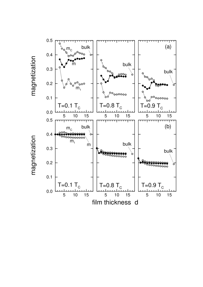
Figure 3: Surface-, center-, and mean magnetization ($m_{1}$, $m_{c}$, $m$) as a function of the film thickness $d$ for three different temperatures $T=0.1\,T_{C}$, $T=0.8\,T_{C}$, and $T=0.9\,T_{C}$; (a) fcc(100); (b) fcc(111). Further parameters: $U=50\,$eV, $t=-0.25\,$eV, $n=1.6$.

We want to emphasize that the finding of a reduced surface magnetization cannot be explained by the well-known Stoner criterion of ferromagnetism. Since the variance of the BDOS is reduced at the surface layer ($\Delta_{s}^{(2)}<\Delta_{b}^{(2)}$, see Tab. 1) due to the reduced coordination number one might intuitively expect the magnetization at the surface to be more robust than in the bulk. However, as discussed in Sect. 1, intensive investigations of strongly correlated electron systems well beyond Hartree-Fock (Stoner) theory clearly point out the importance of a large skewness $\Delta^{(3)}$ for the stability of ferromagnetism [39, 40, 43]. Since the skewness of the BDOS is strongly reduced at the surface (see Tab. 1) this explains the trend of a reduced surface magnetization. The above argument can be checked by considering the BDOS of the surface layer (see. Fig. 1) as an input for an additional MAA calculation. Doing so we find that a “separated” surface layer would be ferromagnetic for the fcc(111) but paramagnetic for the fcc(100) film structure. In this sense the surface layer of an fcc(100) film is magnetized only because of the effective field induced by the ferromagnetically ordered inner layers.

The Curie temperature is found to be unique for the whole film. Note, that although the mean magnetization is reduced for the fcc(100) film with respect to fcc(111) the corresponding Curie temperature is enhanced ($T_{C}^{(100)}(d=5)=1140\,$K, $T_{C}^{(111)}(d=5)=1050\,$K). The inner layers that are fully polarized at $T=0\,$K for both film structures appear to be magnetically more stable for fcc(100) compared to fcc(111). Again, this trend can also be seen in an additional MAA calculation for the BDOS of the respective central layers. The Curie temperatures converge to the corresponding bulk value ($T_{c}^{\textrm{\scriptsize bulk}}=1050\,$K) for $d^{(111)}\approx 3$ and $d^{(100)}\approx 6$.

In Fig. 3 the surface-, center-, and mean magnetization ($m_{1}$, $m_{c}$ and $m$) are shown as a function of the film thickness. The surface magnetization is reduced compared to the mean magnetization. The reduction is weak for fcc(111) films but very pronounced in the case of the fcc(100) structure. This holds not only for thin films where some oscillations are present due to the finite film thickness, but also extends to the limit $d\rightarrow\infty$ where the two surfaces are well separated and do not interact. The oscillations as a function of $d$ which are present for the fcc(100) structure get damped for higher temperatures. One can see from Fig. 3 that the center layer magnetization $m_{c}$ for thick films ($d>10$) is in good agreement with the corresponding fcc bulk calculation [49].

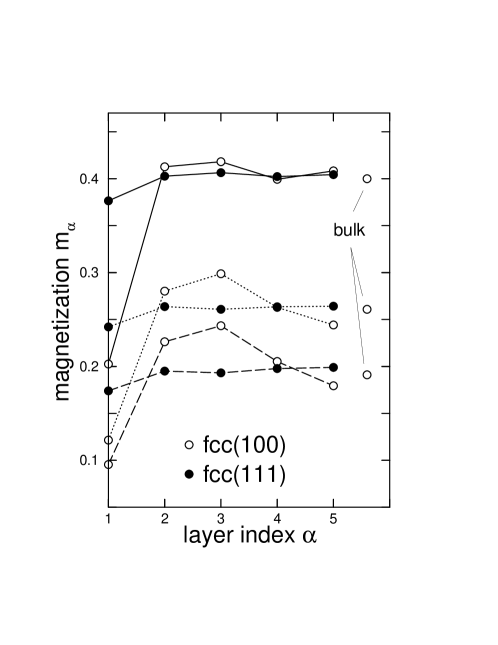
Figure 4: Magnetization profile of a ten layer film for three different temperatures $T=0.1\,T_{C}$ (solid line), $T=0.8\,T_{C}$ (dotted line), and $T=0.9\,T_{C}$ (dashed line). Further parameters: $U=50\,$eV, $t=-0.25\,$eV, $n=1.6$.

The magnetization profile for both film geometries is plotted for $d=10$ in Fig. 4. Here again the magnetizations of the fcc(100) film show a pronounced layer dependence while they are very close to the bulk value from the second layer on in the case of the fcc(111) film geometry. The magnetization profiles are similar to the ones obtained in [21] for Cu/Ni/Cu sandwiches calculated within a single-site spin-fluctuation theory. However, within the present approach the deviation from the bulk magnetization is enhanced close to the Curie temperature for the fcc(100) structure (Fig. 4). Note that a similar trend to a reduced surface magnetization is also found within localized spin models. However, for the uniform Heisenberg model without a layer-dependent anisotropy contribution, the layer magnetizations necessarily increase monotonously from the surface to the central layer [22, 20].

To understand the magnetic behavior on a microscopic basis we will, in the following, discuss the temperature-dependent electronic structure of the thin film systems. For a five layer fcc(100) film the spin- and layer-dependent spectral density at the gamma $\bar{\Gamma}$ point and the quasiparticle density of states are plotted in Fig. 5. There appear two correlation induced band-splittings in the quasiparticle spectrum: Due to the strong Coulomb interaction the spectrum splits into a low and a high energy subband (“Hubbard bands”) which are separated by an energy of the order $U$. Besides this so-called “Hubbard splitting” that is present for all temperatures there is an additional exchange splitting in majority ($\sigma=\uparrow$) and minority ($\sigma=\downarrow$) spin direction for temperatures below $T_{C}$. In the lower subband the electron mainly hops over empty sites, while in the upper subband it hops over lattice sites that are already occupied by another electron with opposite spin. The corresponding weights of the subbands scale with the probability of the realization of these two situations. In the strong coupling limit the scaling is given by $(1-n_{\alpha-\sigma})$ and $n_{\alpha-\sigma}$ for the lower and upper subband, respectively. Since the total band occupation ($n=1.6$) considered here is above half filling, the chemical potential $\mu$ is located in the upper subband while the lower subband is completely filled.

Figure 5: Spectral-density at the gamma point ($\bar{\Gamma}$) and quasiparticle density of states of a five layer FCC(100) Hubbard film. Only the surface layer ($\alpha=1$) and the central layer ($\alpha=3$) are shown. Solid lines: $\sigma=\uparrow$; dotted lines: $\sigma=\downarrow$. The chemical potential is located at zero energy. Further parameters: $U=50\,$eV, $t=-0.25\,$eV, $n=1.6$.

Starting from the Curie temperature the evolution of the quasiparticle spectrum with decreasing temperature is dominated by two distinct correlation effects. Both are driven by an increasing spin-asymmetry in the bandshift $B_{\alpha-\sigma}$. Firstly the centers of gravity of the majority and minority subbands move apart with decreasing temperature (Stoner-type behavior). Secondly there is a strong spin-dependent transfer of spectral weight between the lower and the upper subbands according to the above mentioned scaling, which results in spin- and temperature-dependent widths of the respective subbands. This behavior can also be seen in detail in Fig. 6 and Fig. 7 where the quasiparticle bandstructure of the surface and central layer is plotted for a five layer fcc(100) and fcc(111) film, respectively. Here, only the upper subbands are shown. While the centers of gravity of the upper $\sigma=\downarrow$ subbands are shifted to higher energies for decreasing temperatures, the lowest excitation peak in the spectral density at $\bar{\Gamma}$ is even lowered due to the increasing bandwidth. On the other hand the width of the upper $\sigma=\uparrow$ subband decreases. The interplay of these two correlation effects leads to an inverse exchange splitting at the lower edge of the upper subband near to the $\bar{\Gamma}$ point. The corresponding quasiparticle density of states is, however, very small. Note, that for the same reason the position of the central peak of the upper subband is almost spin- and temperature-independent. This behavior holds for both film structures for ${\bf k}$-vectors not too far away from $\bar{\Gamma}$.

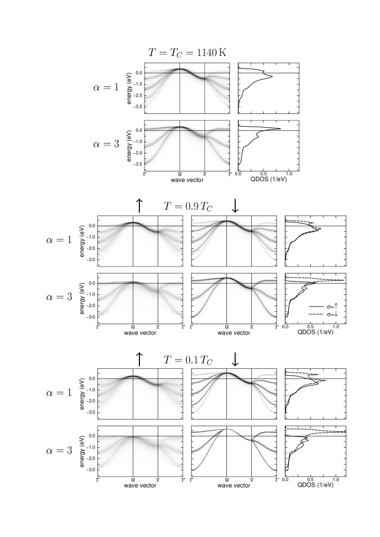
Figure 6: Spin- and layer- dependent spectral density and quasiparticle density of states of a five layer fcc(100) film for three different temperatures $T=0.1\,T_{C}$, $T=0.9\,T_{C}$, and $T=T_{C}$. Only the upper Hubbard band is shown. $\alpha=1$: surface layer; $\alpha=3$: central layer. The chemical potential is located at zero energy. Further parameters: $U=50\,$eV, $t=-0.25\,$eV, $n=1.6$.

With help of the quasiparticle bandstructure given in Fig. 6 and Fig. 7 the exchange splitting between majority and minority spin direction can be analyzed in more detail. For both film structures the exchange splitting is wavevector-dependent. It is strongest near $\bar{M}$ for fcc(100) and between $\bar{M}$ and $\bar{K}$ for fcc(111). Contrary to the fcc(100) structure all layers are fully polarized at $T=0\,$K for the fcc(111) film. In the case of ferromagnetic saturation the exchange splitting can be estimated [48] to be at most $(1-n_{\alpha\downarrow})[4t-B_{\alpha\downarrow}]$, where $(1-n_{\alpha\downarrow})B_{\alpha\downarrow}$ is the effective bandshift between the centers of gravity of the upper quasiparticle subbands. For strong Coulomb interaction $n_{\alpha\downarrow}(1-n_{\alpha\downarrow})B_{\alpha\downarrow}$ is proportional to the kinetic energy [47] of the $\sigma=\downarrow$ electrons in the $\alpha$-th layer. Note that the kinetic energy of the $\sigma=\uparrow$ electrons vanishes for the ferromagnetic saturated state since the $\sigma=\uparrow$ band is completely filled. We want to point out that these results strongly contrast the findings of Hartree-Fock theory where the exchange splitting is wavevector-independent and proportional to $m_{\alpha}U$ leading to substantially higher Curie temperatures compared to the MAA. The temperature-dependence of the electronic structure within the MAA is completely different to the Stoner picture of ferromagnetism.

Let us discuss the quasiparticle lifetime which corresponds to the width of the quasiparticle peaks. From the spectral density (Figs. 5, 6, 7) one can clearly read off that the lifetime of the quasiparticles is strongly spin- and temperature-dependent. For low temperatures the upper minority spectrum is sharply peaked which indicates long living quasiparticles. This is due to the fact that in the ferromagnetic saturated state a $\sigma=\downarrow$ electron does meet a $\sigma=\uparrow$ electron at any lattice site and thus effectively does not perform any scattering process. The width of the $\sigma=\uparrow$ quasiparticle peaks, however, is broadened for decreasing temperature. Thus in the majority spectrum the quasiparticle lifetime decreases for increasing magnetization. What concerns the lower subbands (see Fig. 5) the respective spectrum is strongly damped and the different excitations due to the five layer structure are almost indistinguishable.

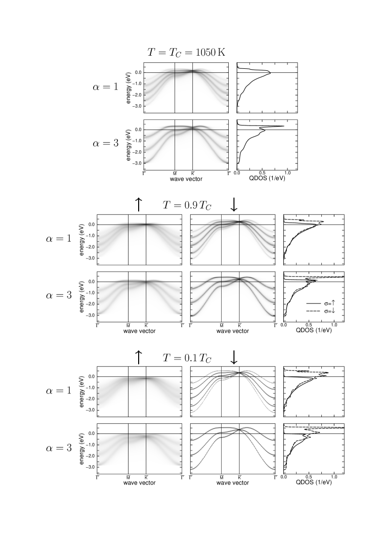
Figure 7: Spin and layer dependent spectral density and quasiparticle density of states of a five layer fcc(111) film for three different temperatures $T=0.1\,T_{C}$, $T=0.9\,T_{C}$, and $T=T_{C}$. Only the upper Hubbard band is shown. $\alpha=1$: surface layer; $\alpha=3$: central layer. The chemical potential is located at zero energy. Further parameters: $U=50\,$eV, $t=-0.25\,$eV, $n=1.6$.

For given spin and wavevector the positions of the quasiparticle peaks are layer-independent. In principle, their number corresponds to the number of layers of the film. However, due to symmetry some peaks are left out for certain layers. For thicker films the different peaks move closer together as their number increases until they build a continuum for $d\rightarrow\infty$ which corresponds to the projection of the three dimensional bandstructure onto the surface Brillouin zone. Between $\bar{M}$ and $\bar{X}$ for fcc(100) and at $\bar{K}$ for fcc(111) the different peaks merge together due to vanishing interlayer hopping ($\gamma_{\perp}({\bf k})=0$).

In Figs. 6, 7 the QDOS of the surface and central layer are shown additionally. The Van Hove singularities resulting from the different branches of the quasiparticle dispersion are clearly visible. There are sharp Van Hove singularities in the minority spectrum while they are broadened for the majority spin direction because of the finite widths of the $\sigma=\uparrow$ quasiparticle peaks due to the quasiparticle damping.

Finally we want to stress that the results presented above do not depend on the size of the Coulomb interaction $U$ as long as $U$ is chosen from the strong-coupling region ($U\gg W$). Contrary to Hartree-Fock theory, all magnetic key quantities like the Curie temperature and the exchange splitting saturate as a function of $U$. On the other hand, although the MAA was optimized with respect to the strong coupling limit we believe that, at least qualitatively, the correlation effects in the spin-, layer-, and temperature-dependent electronic structure are valid down to intermediate Coulomb interaction as well.

6 Conclusion

For the investigation of spontaneous ferromagnetism and electron correlation effects in thin itinerant-electron films we have applied a generalization of the modified alloy analogy (MAA) to the single-band Hubbard model with reduced translational symmetry. The MAA is based on the alloy analogy concept and is optimized with respect to correct strong coupling behavior [44, 45]. Within the MAA the actual type of the underlying alloy is not predetermined but has to be determined selfconsistently. In this sense the MAA is able to account for the itineracy of the $-\sigma$ electrons which are considered as strictly “frozen” in the conventional alloy analogy (AA). In the paramagnetic phase MAA and AA are almost identical. However, contrary to the AA spontaneous ferromagnetic order is possible for special parameter constellations within the MAA. With help of the MAA the interplay of magnetism and quasiparticle damping effects can be studied in a natural way.

For an fcc(100) and an fcc(111) film geometry the layer-dependent magnetizations have been discussed as a function of temperature as well as film thickness. The magnetization in the surface layer is found to be reduced with respect to the inner layers for all thicknesses and temperatures considered. While this reduction is weak for fcc(111) films it is pronounced in the case of an fcc(100) geometry. The effect of the surface is considerably stronger for fcc(100) films due to the higher percent of missing nearest neighbor atoms. The reduction of the surface layer magnetization is not to be expected within an Hartree-Fock type approach (Stoner criterion) to the Hubbard film being, therefore, a genuine effect induced by strong electron correlations.

The magnetic behavior of the thin film systems can be microscopically understood by means of the spin- layer- and temperature- dependent quasiparticle bandstructure and the corresponding quasiparticle density of states. There appear two correlation induced band splittings in the quasiparticle spectrum. Besides the Hubbard splitting there is an additional exchange splitting for temperatures below $T_{C}$. The demagnetization process as a function of temperature is dominated by two distinct correlation effects: A Stoner-like shift in the centers of gravity of the majority and minority subbands together with a strong spin-dependent transfer of spectral weight between the upper and lower subbands. An interplay of these two effects results in Curie temperatures far below the corresponding Hartree-Fock values. The exchange splitting is found to be strongly wavevector-dependent and is substantially different for the various quasiparticle branches in the bandstructure. The widths of the quasiparticle peaks that correspond to the quasiparticle lifetime exhibit a strong spin- and temperature-dependence. For $T=0\,$K the minority-spin quasiparticle peaks are sharply peaked while the majority-spin spectrum is substantially broadened.

Clearly the degeneracy of the 3d-bands has to be included if a direct comparison to the experiment is intended. Within the present scheme this could be achieved by a similar approach as presented in [33] which is planed for the future. However we believe the correlation effects found here to be important within a generalized Hubbard model as well. In this work we have exclusively focused on purely ferromagnetic films. In addition one can examine within the same theory a phase with antiferromagnetic order between the layers. We expect such a situation to exist close to half-filling ($n=1$) and for intermediate values of the Coulomb interaction. Further the influence of a non-magnetic top layer on the magnetic behavior of thin films can be investigated.

References

References

- [1] R. Allenspach, J. Magn. Magn. Mat. 129, 160 (1994).
- [2] K. Baberschke, Appl. Phys. A 62, 417 (1996).
- [3] H. J. Elmers, Int. J. Mod. Phys. B 9, 3115 (1995).
- [4] M. Getzlaff, J. Bansmann, J. Braun, and G. Schönhense, Z. Phys. B 104, 11 (1997).
- [5] W. Dürr, M. Taborelli, O. Paul, R. Germar, W. Gudat, D. Pescia, and M. Landolt, Phys. Rev. Lett. 62, 206 (1989).
- [6] D. P. Pappas, K.-P. Kämper, and H. Hopster, Phys. Rev. Lett. 64, 3179 (1990).
- [7] M. Farle, W. Platow, A. N. Anisimov, P. Poulopoulos, and K. Baberschke, Phys. Rev. B 56, 5100 (1997).
- [8] C. L. Fu and A. J. Freeman, Phys. Rev. B 35, 925 (1987).
- [9] T. Kraft, P. M. Marcus, and M. Scheffler, Phys. Rev. B 49, 11511 (1995).
- [10] T. Asada and S. Blügel, Phys. Rev. Lett. 79, 507 (1997).
- [11] R. Lorenz and J. Hafner, Phys. Rev. B 54, 15937 (1996).
- [12] D. Spišák and J. Hafner, Phys. Rev. B 56, 2646 (1997).
- [13] D. Reiser, J. Henk, H. Gollisch, and R. Feder, Solid State Commun. 93, 231 (1995).
- [14] M. P. Gokhale and D. L. Mills, Phys. Rev. B 49, 3880 (1994); M. Plihal and D. L. Mills, Phys. Rev. B 52, 12813 (1995).
- [15] M. Potthoff and W. Nolting, Surf. Sci. 377-379, 457 (1997).
- [16] T. Herrmann, M. Potthoff, and W. Nolting, Phys. Rev. B 58, 831 (1998).
- [17] N. D. Mermin and H. Wagner, Phys. Rev. Lett. 17, 1133 (1966).
- [18] M. Bander and D. L. Mills, Phys. Rev. B 38, 12015 (1988).
- [19] A.-M. Daré and Y. M. Vilk anf A.-M. S. Tremblay, Phys. Rev. B 53, 14236 (1996).
- [20] R. Schiller and W. Nolting, to be published (1998).
- [21] H. Hasegawa, Surf. Sci. 182, 591 (1987).
- [22] W. Haubenreisser, W. Brodkorb, A. Corciovei, and G. Costache, phys. stat. sol. (b) 53, 9 (1972); D. T. Hung, J.C. S. Levy, and O. Nagai, phys. stat. sol. (b) 93, 351 (1979).
- [23] R. P. Erickson and D. L. Mills, Phys. Rev. B 43, 10715 (1991); R. P. Erickson and D. L. Mills, Phys. Rev. B 44, 11825 (1991).
- [24] P. J. Jensen, H. Dreyssé, and K. H. Bennemann, Surf. Sci. 269/270, 627 (1991).
- [25] Long-Pei Shi and Wei-Gang Yang, J. Phys.: Condens. Matter 4, 7997 (1992).
- [26] A. Hucht and K. D. Usadel, Phys. Rev. B 55, 12309 (1997).
- [27] P. J. Jensen and K. H. Bennemann, Solid State Commun. 105, 577 (1998).
- [28] J. Hubbard, Proc. R. Soc. London, Ser. A 276, 238 (1963); M. C. Gutzwiller, Phys. Rev. Lett. 10, 159 (1963); J. Kanamori, Prog. Theor. Phys. (Kyoto) 30, 275 (1963).
- [29] J. Hubbard, Proc. R. Soc. London, Ser. A 277, 237 (1964).
- [30] D. Vollhardt, N. Blümer, K. Held, J. Schlipf, and M. Ulmke, Z. Phys. B 103, 283 (1997).
- [31] K. Held and D. Vollhardt, to appear in Eur. Phys. J. B (1998), cond–mat/9803182.
- [32] T. Momoi and K. Kubo, Phys. Rev. B 58, R567 (1998).
- [33] W. Nolting, W. Borgieł, V. Dose, and Th. Fauster, Phys. Rev. B 40, 5015 (1989); W. Nolting, A. Vega, and Th. Fauster, Z. Phys. B 96, 357 (1995); A. Vega and W.Nolting, phys. stat. sol. (b) 193, 177 (1996).
- [34] A. Haroun, A. Chouairi, S. Ouannasser, H. Dreyssé, G. Fabricius, and A.M. Llois, Surf. Sci. 307-309, 1087 (1994).
- [35] J. Dorantes-Dávila, H. Dreyssé, and G. M. Pastor, Phys. Rev. B 55, 15033 (1997).
- [36] H. Hasegawa, J. Phys.: Condens. Matter 4, 1047 (1992).
- [37] M. Ulmke, Eur. Phys. J. B 1, 301 (1998).
- [38] G. S. Uhrig, Phys. Rev. Lett. 77, 3629 (1996).
- [39] Th. Hanisch and G. Uhrig. E. Müller-Hartmann, Phys. Rev. B 56, 13960 (1997).
- [40] J. Wahle, N. Blümer, J. Schlipf, K. Held, and D. Vollhardt, Phys. Rev. B 58, 12749 (1998).
- [41] T. Obermaier, T. Pruschke, and J. Keller, Phys. Rev. B 56, 8479 (1997).
- [42] T. Herrmann and W. Nolting, Solid State Commun. 103, 351 (1997).
- [43] M. Potthoff, T. Herrmann, T. Wegner, and W. Nolting, phys. stat. sol. (b) 210, 199 (1998).
- [44] A. B. Harris and R. V. Lange, Phys. Rev. 157, 295 (1967).
- [45] H. Eskes and A. M. Oleś, Phys. Rev. Lett. 73, 1279 (1994); H. Eskes, A. M. Oleś, M. B. J. Meinders, and W. Stephan, Phys. Rev. B 50, 17980 (1994).
- [46] W. Nolting and W. Borgieł, Phys. Rev. B 39, 6962 (1989).
- [47] T. Herrmann and W. Nolting, J. Magn. Magn. Mat. 170, 253 (1997).
- [48] T. Herrmann and W. Nolting, Phys. Rev. B 53, 10579 (1996).
- [49] W. Nolting and T. Herrmann, Condensed Matter Theories 13, 169 (1998).
- [50] M. Potthoff, T. Herrmann, and W. Nolting, Eur. Phys. J. B 4, 485 (1998).
- [51] M. Potthoff and W. Nolting, J. Phys.: Condens. Matter 8, 4937 (1996).
- [52] J. Hubbard, Proc. R. Soc. London, Ser. A 281, 401 (1964).
- [53] B. Velický, S. Kirkpatrick, and H. Ehrenreich, Phys. Rev. 175, 747 (1968).
- [54] R. Vlamming and D. Vollhardt, Phys. Rev. B 45, 4637 (1992).
- [55] J. Schneider and V. Drchal, phys. stat. sol. (b) 68, 207 (1975).