Orbital dynamics in ferromagnetic transition metal oxides
Abstract
We consider a model of strongly correlated electrons interacting by superexchange orbital interactions in the ferromagnetic phase of LaMnO3. It is found that the classical orbital order with alternating occupied orbitals has a full rotational symmetry at orbital degeneracy, and the excitation spectrum derived using the linear spin-wave theory is gapless. The quantum (fluctuation) corrections to the order parameter and to the ground state energy restore the cubic symmetry of the model. By applying a uniaxial pressure orbital degeneracy is lifted in a tetragonal field and one finds an orbital-flop phase with a gap in the excitation spectrum. In two dimensions the classical order is more robust near the orbital degeneracy point and quantum effects are suppressed. The orbital excitation spectra obtained using finite temperature diagonalization of two-dimensional clusters consist of a quasiparticle accompanied by satellite structures. The orbital waves found within the linear spin-wave theory provide an excellent description of the dominant pole of these spectra.
pacs:
PACS numbers: 71.27.+a, 75.10.Jm, 75.30.Ds, 75.40.Gb.I Introduction
Recently much attention has been attracted to the properties of La1-xAxMnO3, with A=Ca,Sr,Ba, and related compounds, in which the colossal magnetoresistance and metal-insulator transition are observed.[2] The parent compound, LaMnO3, is insulating with layered-type antiferromagnetic (AF) ordered state (the A-type antiferromagnet), accompanied by the orbital order with alternation of orbitals occupied by a single electron of Mn3+ ions.[3] Such orbitally ordered states might be promoted by a cooperative Jahn-Teller effect,[4] playing a decisive role in charge transport,[5] but could also result from an electronic instability.[6] The latter possibility is now under debate, as the band structure calculations performed within the extension of local density approximation (LDA) to strongly correlated transition metal oxides, the so-called LDA+U approach, give indeed charge-ordered ground states without assuming lattice distortions as their driving force.[7] Charge ordering was also found within the Hartree-Fock calculations on lattice models by Mizokawa and Fujimori.[8]
The dominating energy scale in late transition metal oxides is the local Coulomb interaction between electrons at transition metal ions which motivates the description of ground state and low-energy excitations in terms of effective models with spin and orbital degrees of freedom. Such models, introduced both for the cuprates,[9, 10] and more recently for the manganites,[11, 12, 13] show that the spin and orbital degrees of freedom are interrelated which leads to an interesting problem, even without doping. Orbital interactions in the ground state lead to a particular orbital ordering that depends on the magnetic ordering, and vice versa. An interesting aspect of such system is that the elementary excitations have either a pure spin, or pure orbital, or mixed spin-orbital character.[14, 15, 16] This gives large quantum fluctuation corrections to the order parameter in AF phases, and it was discussed recently that this might lead to a novel type of a spin-liquid.[10, 17, 14] In a special case of ferromagnetic (FM) order (which represents a simplified spinless problem), only orbital excitations contribute to the properties of the ground state and the quantum effects are expected to be smaller.
Unlike in the cuprate materials, hole doping in the manganites leads to FM states, insulating at low doping, and metallic at higher doping.[18] Although the FM phase is unstable for the undoped LaMnO3, the building blocks are FM planes. A proper understanding of pure orbital excitations has to start from the uniform FM phase, where the spin operators can be integrated out. Such a state could possibly be realized in LaMnO3 at large magnetic field and will serve as a reference state to consider hole propagation in doped manganites, similarly as the AF spin state provides a reference state for the hole propagation in the cuprates. Therefore, we consider in this paper an effective model with only orbital superexchange interactions which involves the states and results from the effective Hamiltonians derived in Refs. [10, 11, 12, 13] in the relevant high-spin state. Of course, it is identical for the cuprates and for the manganites. We note, however, that orbital interactions may be also induced by lattice distortions, but these contributions are expected to be less important than the orbital superexchange,[19] and will be neglected.
So far, little is known about the consequences of orbital excitations for long-range order and transport properties in doped systems, but it might be expected that such excitations either bind to a moving hole, or lead to hole scattering even when the spins are aligned.[20] The knowledge of orbital excitations is a prerequisite for a better understanding of the temperature dependence of the resistivity and optical conductivity in the FM phase of doped manganites. Although the double exchange mechanism is quite successful in explaining why the spin order becomes FM with increasing doping of La1-xAxMnO3, it fails to reproduce the experimentally observed temperature dependence of the resistivity.[21] Even more puzzling and contradicting naive expectations is the incoherent optical conductivity with a small Drude peak observed in a FM metallic phase at higher doping.[22] This behavior demonstrates the importance of orbital dynamics in doped manganites which appears to be predominantly incoherent in the relevant parameter regime.[23, 24]
The paper is organized as follows. The orbital superexchange model is presented in Sec. II. We derive the classical phases with alternating orbitals on two sublattices in three and two dimensions, and analyze their dependence on the crystal field splitting. Orbital excitations are derived in Sec. III using a pseudospin Hamiltonian and an extension of the linear spin-wave theory (LSWT) to the present situation with no conservation of orbital quantum number. We present numerical results for the dispersion of orbital waves and determine quantum fluctuation corrections to the ground-state energy and to the order parameter in Sec. IV. The derived spectra are compared with the results of exact diagonalization in Sec. V. A short summary and conclusions are given in Sec. VI.
II Orbital Hamiltonian and classical states
A Orbital superexchange interactions
We consider a three-dimensional (3D) Mott insulator with one electron per site. The effective Hamiltonian which describes electrons in a cubic crystal at strong-coupling,[10, 11, 12, 13]
| (1) |
consists of the superexchange part , and the orbital splitting term due to crystal-field term . Here we will consider a special case of the FM band in which the spin dynamics is integrated out and one is left with the effective interactions between the electrons (holes) in different orbital states. In this case the only superexchange channel which contributes is the effective interaction via the high-spin state, and thus the interaction occurs only between the pairs of ions with singly occupied orthogonal orbitals at two nearest-neighbor sites (two orthogonal orbitals are then singly occupied in the intermediate excited states). An example of such a model is the superexchange interaction in the FM state of LaMnO3 which originates from excitations (with , , and ) into a high-spin state , as shown schematically in Fig. 1. It gives the effective Hamiltonian with orbital interactions,[12, 13]
| (2) |
where is the hopping element between the directional orbitals along the considered -axis, and is the excitation energy. The orbital degrees of freedom are described by the projection operators which select a pair of orbitals and , being parallel and orthogonal to the directions of the considered bond in a cubic lattice.
The Hamiltonian (2) has cubic symmetry and may be written using any reference basis in the subspace. For the conventional choice of and orbitals, the above projection operators are represented by the orbital operators , with for three cubic axes,
| (3) |
It is convenient to replace the orbital operators by the pseudospin operators with ,
| (4) |
The latter operators may be represented by the Pauli matrices in the same way as spin operators, , and obey the same commutation relations. Therefore, the th component of pseudospin is given by , and we identify the orbital states as up- and down-pseudospin, , and , respectively. We take the prefactor in Eq. (2) as the energy unit for the superexchange interaction. Thus, one finds a pseudospin Hamiltonian,
| (5) | |||||
| (6) |
where the prefactor of the mixed term is negative in the -direction and positive in the -direction.[25] We choose a convention that the bonds labeled as () connect nearest-neighbor sites within planes (along the -axis). The virtual excitations which lead to the interactions described by Eq. (6) are shown in Fig. 1. Here we neglected a trivial constant term which gives the energy of per bond, i.e., per site in a 3D system. We emphasize that the symmetry is explicitly broken in , and the interaction depends only on two pseudospin operators, and .
The crystal-field term removes the degeneracy of and orbitals,
| (7) |
and is connected with the uniaxial pressure. This term is induced by static distortions in a tetragonal field and is of particular importance in a two-dimensional (2D) system.
B Classical ground states
Before analyzing the excitation spectra of the Hamiltonian (6), one has to determine first the classical ground state of the system that will serve as a reference state to calculate the Gaussian fluctuations. Neglecting the irrelevant phase factors, the classical configurations which minimize the interaction terms (6) are characterized by the two-sublattice pseudospin order, with two angles describing orientations of pseudospins, one at each sublattice. As usually, the classical ground state is obtained by minimizing the energy with respect to these two rotation angles, i.e., by choosing the optimal orbitals.
Let us consider first the term at orbital degeneracy . The superexchange interaction (2) induces the alternation of orthogonal orbitals in the ground state in all three directions, and is equivalent to the two-sublattice AF (G-AF) order in the pseudospin space. This configuration gives the lowest energy on the mean-field level, as the virtual transitions represented in Fig. 1 give the largest contribution, if the hopping involves one occupied and one unoccupied orbital of the same type (e.g., either directional or planar). A priori, the optimal choice of the occupied orbitals could be unique on the classical level due to the cubic symmetry of superexchange interaction (2). Therefore, we perform a uniform rotation of orbitals by an angle at each site,
| (8) |
to generate the new orthogonal orbitals, and , and investigate the energy as a function of . The AF order imposed by the Hamiltonian in a cubic system implies the alternation of these orthogonal orbitals in the rotated basis, and , at two sublattices, i.e., and . A few examples of various possible choices of the orthogonal orbitals are given in Table I for representative values of .
The rotation (8) leads to the following transformation of the pseudospin operators,
| (9) | |||||
| (10) |
and the interaction Hamiltonian is then transformed into,
| (11) |
| (14) | |||||
| (16) | |||||
As in Eq. (6), the bonds in the first sum (14) are parallel to either or -axis, while the bonds in the second sum (16) are parallel to the -axis. The classical energy is minimized if , i.e., if the orbitals order ’antiferromagnetically’.
The Hamiltonian given now by Eqs. (14) and (16) has the symmetry of the cubic lattice, but surprisingly one finds the full rotational symmetry of the present interacting problem on the classical level at orbital degeneracy. In other words, classically the lowest energy is always per site, independent of the rotation angle, as long as alternating orbitals on neighboring sites are occupied. This follows from the particular structure of the rotated Hamiltonian (11) which has identical factors of three in front of the diagonal and off-diagonal contributions, when these are summed over all the bonds which originate at each site, and these coefficients are independent of the rotation angle . In contrast to the Heisenberg antiferromagnet (HAF), however, this symmetry concerns only the summed contributions, and not the interactions along the individual bonds.
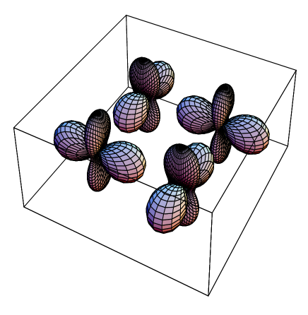
A finite orbital field breaks the rotational symmetry on the classical level. It acts along the -axis, and it is therefore easy to show that the ground state in the limit of is realized by the alternating occupied orbitals being symmetric/antisymmetric linear combinations of and orbitals,[13] i.e., the occupied states correspond to the rotated orbitals (8) and on the two sublattices with an angle , shown in Fig. 2 (see also Table I). In particular, this state is different from the alternating directional orbitals, and , which might have been naively expected. It follows in the limit of degenerate orbitals from the ’orbital-flop’ phase, in analogy to a spin-flop phase for the HAF at finite magnetic field. With increasing (decreasing) the orbitals tilt out of the state shown in Fig. 2, and approach orbitals, respectively, which may be interpreted as an increasing FM component of the magnetization in the pseudospin model.
It is convenient to describe this tilting of pseudospins due to the crystal-field by making two different transformations (8) at both sublattices, rotating the orbitals by an angle on sublattice , and by an angle on sublattice , so that the relative angle between the occupied orbitals is and decreases with increasing , i.e., with increasing ,
| (17) |
| (18) |
As before, the orbitals and are occupied at two sublattices, and , respectively, and the orbital order is AF in the classical state, with the transformed operators and , respectively. As a result one finds that the angles for the occupied orbitals are indeed opposite on the two sublattices.
The operators and may be now transformed as in Eqs. (10) using the actual rotations by , as given in Eqs. (17) and (18), and the transformed Hamiltonian takes the form,
| (19) |
| (22) | |||||
| (24) | |||||
| (25) |
where for and for . The energy of the classical ground state is given by,
| (26) |
and is minimized by,
| (27) |
At orbital degeneracy () this result is equivalent to () in Eq. (8), as obtained also in Ref. [13], and one recovers from Eq. (26) the energy of as a particular realization of the degenerate classical phases with alternating orthogonal orbitals. The above result (27) is valid for ; otherwise one of the initial orbitals (either or ) is occupied at each site, and the state is fully polarized (). The case of corresponds to the occupied orthogonal orbitals at orbital degeneracy. In contrast, the value of corresponds to performing no rotation on the sublattice, while the orbitals are interchanged on the sublattice [see Eqs. (17) and (18)]. The latter situation describes a state obtained in strong orbital field, with only one type of orbitals occupied, a ’FM orbital state’. The orbital field changes therefore the orbital ordering from the AF to FM one in a continuous fashion.
C Two-dimensional orbital model
As a special case we consider also a 2D orbital model with the interactions in the plane. In this case the cubic symmetry is explicitly broken, and the classical state is of a spin-flop type. It corresponds to alternatingly occupied orbitals on the two sublattices, with the orbitals oriented in the plane and given by at , see Fig. 2.[26] A finite value of tilts the orbitals out of the planar orbitals by an angle , and the Hamiltonian reduces to
| (28) |
as there is no bond in the -direction. The classical energy is
| (29) |
Therefore, one finds the same energy of as in a 3D model at orbital degeneracy. This shows that the orbital superexchange interactions are geometrically frustrated, and the bonds in the third dimension cannot lower the energy, but only allow for restoring the rotational symmetry on the classical level and rotating the orthogonal orbitals in an arbitrary way. The energy (29) is minimized by,
| (30) |
if ; otherwise . Interestingly, the value of the field at which the orbitals are fully polarized is reduced by one third from the value obtained in three dimensions (27). This shows that although the orbital exchange energy can be gained in a 3D model only on the bonds along two directions in the alternating (orbital-flop) phase either at or close to , one has to counteract the superexchange on the bonds in all three directions when the field is applied.
We note that the present orbital model becomes purely classical in one dimension, if the lattice effects are neglected, as we have assumed in the present model. This follows from the derivation which gives the superexchange interactions of Ising type between the orbitals along the -axis, and one can always choose this axis along the considered chain. Thus, one finds the Hamiltonian
| (31) |
At orbital degeneracy () the occupied orbitals alternate along the one-dimensional (1D) chain between two orthogonal orbitals, and one may for example choose the occupied states as and on even and odd sites, respectively. The energy of this ground state per site is , which allows to conclude that energy gains due to orbital ordering per site are significantly reduced compared to the 2D and 3D case.
III Orbital excitations in linear spin-wave theory
The superexchange in the orbital subspace is AF and one may map the orbital terms in the Hamiltonian (6) onto a spin problem in order to treat the elementary excitations within the LSWT. The equations of motion can then be linearized by a standard technique.[4] Let us first discuss the results of LSWT for the spin-flop phase induced by an orbital-field, starting from the rotated Hamiltonian (19). Here we choose the Holstein-Primakoff transformation [27] for localized pseudospin operators (),
| (32) | |||||
| (33) |
for sublattice and
| (34) | |||||
| (35) |
for sublattice. After replacing the square roots by the leading lowest order terms, and inserting the expansion into Eq. (19), one diagonalizes the linearized Hamiltonian by two consecutive transformations. Note that, contrary to the HAF, also cubic terms in boson operators are present in the expansion due to the anomalous interactions .
The linearized Hamiltonian simplifies by introducing the Fourier transformed boson operators and given by,
| (36) |
and by transforming to new boson operators ,
| (37) |
One finds the effective orbital Hamiltonian of the form,
| (38) | |||||
| (39) |
where the coefficients and depend on angle ,
| (40) | |||||
| (41) |
and the -dependence is given by , and by , respectively. After a Bogoliubov transformation,
| (42) |
with the parameters
| (43) |
with , and an equivalent transformation for the bosons, the Hamiltonian (39) is diagonalized, and takes the following form,
| (44) |
The orbital-wave dispersion is given by
| (46) | |||||
The orbital excitation spectrum consists of two branches like, for instance, in an anisotropic Heisenberg model.[28]
The dependence on the field is implicitly contained in the above relations via the angle , as determined by Eqs. (27) and (30) for the 3D and 2D model, respectively. The dispersion changes between the case of () which stands for the spin-flop phase at orbital degeneracy, and the case of () which corresponds to the uniform phase with either () or () orbitals occupied. The orbital field therefore changes the orbital-wave dispersion from AF to FM state. The orbital-wave dispersion for a 2D system, can easily be found from Eq. (46) by setting .
In the case of a vanishing orbital field the classical ground state is degenerate with respect to a rotation of the orbital around an arbitrary angle . In LSWT, nevertheless, the orbital-wave dispersion depends on , i.e., the orbital-wave velocity is highly anisotropic, and one finds,
| (47) | |||||
| (48) |
with respectively. It is straightforward to verify that the excitations are gapless, independent of the rotation angle. If , the orbital-waves given by Eq. (46) take a particularly simple form, and is identical to the dispersion found in the spin-flop phase at ,
| (50) |
In both cases the system is quasi-2D and the dispersion originates only from the planar components and .
IV Numerical results
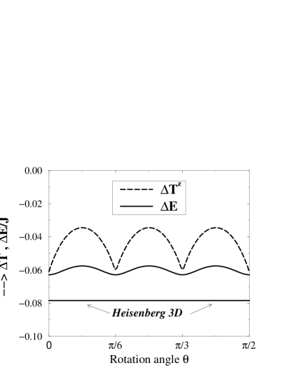
The excitation spectra given by Eq. (46) for different crystal-field splittings are shown in Fig. 3 for the 3D system along different directions of the fcc Brillouin zone [29] appropriate for the alternating orbital order. Most interestingly, a gapless orbital-wave excitation is found for the 3D system at orbital degeneracy. Obviously this is due to the fact that the classical ground state energy is independent of the rotation angle at , as we have shown in Sec. II. At first glance, however, one does not expect such a gapless mode, as the Hamiltonian (6) does not obey a continuous symmetry. The cubic symmetry of the model, however, is restored if one includes the quantum fluctuations; they are shown in Fig. 4 as functions of the rotation angle . Note that the quantum corrections are small and comparable to those of the 3D HAF. They do depend on the rotation angle, as the orbital-wave dispersion does. If the dispersion is completely 2D-like, , corresponding to (50), the quantum corrections are largest, as this dispersion has a line of nodes along the direction, i.e., for .
It is interesting to note that this fully 2D orbital-wave dispersion leads to an orbital ordered state at zero temperature only. At any finite temperature fluctuations destroy the long-range order (as in the 2D HAF). In this way one finds an orbital-liquid state at non-zero temperature, similar to that obtained in a Schwinger-boson approach by Ishihara, Yamanaka and Nagaosa for the doped system.[30] In higher order spin-wave theory, however, it might very well be that a gap occurs in the excitation spectrum. We expect, however, that this gap, if it arises, is small, with its size being proportional to the size of quantum fluctuations.
The cubic symmetry of the model at is satisfied by the quantum-corrected ground-state energy (Fig. 4), as the energy is invariant under rotations by any angle , where is any natural number. This can be expected as such a rotation corresponds to merely directing the orbitals along different cubic axes and/or interchanging the sublattices and .
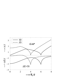
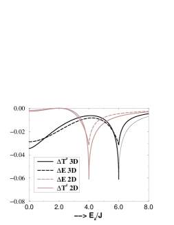
At finite values of the spectrum becomes gapped (Fig. 5) because the degeneracy of the classical ground state is removed. Note that this is different from a HAF in a finite magnetic field, because there one still has full continuous symmetry in the spin-flop phase with respect to rotations along the field axis, which justifies the existence of a Goldstone mode. For small orbital fields the gap firstincreases up to a maximum reached at (), while for larger values the gap decreases and vanishes at () for a 3D (2D) model. This can be understood by making the analogy with an AF Ising model in a magnetic field. As the field increases, the energy of a spin-flip excitation decreases as the loss of interaction energy associated with this excitation is partly compensated by the energy gain due to the parallel alignment of the excited spin to the field. Approaching the phase transition from the spin-flop to FM ordering, this mode becomes softer and is found atzero energy exactly at the transition point. The increase of the gap for is therefore due to a complete FM alignment of the orbitals along the field axis in this parameter regime, and any excitation acts then against the orbital field. In Fig. 6 also the quantum corrections to the ground-state energy and the order parameter are shown as functions of the orbital field. As expected, the presence of a gap in the excitation spectrum suppresses quantum fluctuations.
The quasi-2D state, i.e., the alternation of and on two sublattices, is destabilized by any finite orbital field . Taking for instance , the orbital field shifts downwards the energy of the occupied orbitals on one sublattice by , while the energy of orbitals increases by on the other sublattice, so that the orbital field does not lower the energy of the system. Therefore, the state with is selected instead for the classical ground state for any non-zero orbital field[31] because in this state the pseudospins can tilt towards the orbital field, reducing the energy of the system. Such orbitals forming the ground state are shown in Fig. 2.
The dispersion for the unrotated state suggests that the effective dimensionality of the system is reduced from three to effectively two dimensions in the absence of an orbital splitting. This anisotropy results in overall smaller quantum fluctuations in a 3D model at than in the corresponding HAF, as discussed above. The anisotropy of the 3D model manifests itself in the energy contribution coming from the bonds in the plane and along the -axis, as shown in Fig. 7. For the classical energy along the chain is zero, and the orbital superexchange energy of is gained by the planar bonds. One finds that quantum contributions to the ground-state energy tend to decrease the energy stored in the bonds along the chain, and increase the energy in the plane.
For the 2D system the situation at orbital degeneracy is quite different (see Fig. 3). The lack of interactions along the -axis breaks the symmetry of the model already at , opens a gap in the excitation spectrum and suppresses quantum fluctuations. Increasing the orbital field, however, the system resembles the behavior of a 3D system, where also the gap closes at an orbital field which compensates the energy loss due to the orbital superexchange between identical (FM) orbitals. At this value of the field (), the full dispersion of the orbital waves is recovered, see Fig. 3, the spectrum is gapless, and the quantum fluctuations reach a maximal value. We would like to emphasize that this behavior is qualitatively different from the HAF, where the anomalous terms and are absent, and quantum fluctuations vanish at the crossover from the spin-flop to FM phase.
V Comparison with exact diagonalization in a 2D cluster
It is instructive to make a comparison between the analytic approximations of Sec. III and the exact diagonalization of 2D finite clusters using the finite temperature diagonalization method.[32] In contrast to the mean-field approach presented in Sec. II, one finds a unique ground state at by exact diagonalization, and no rotation of the basis has to be made to investigate the stability of the ground state. Making the rotation of the basis (8) is however still useful in exact diagonalization as it gives more physical insight into the obtained correlation functions which become simpler and more transparent when calculated within an optimized basis. Moreover, they offer a simple tool to compare the results obtained by exact diagonalization with those of the analytic approach, presented in Sec. IV. We shall present below the results obtained with clusters; similar results were also found for 10-site clusters.
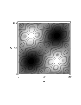
First we calculate nearest-neighbor correlation function in the ground state , where the operators with a tilde refer to a rotated basis,
| (51) | |||||
| (52) |
so that the correlation function depends on two angles: and .
In Fig. 8 the intersite orbital correlation in the ground state is shown as a contour-plot. White (dark) regions correspond to positive (negative) values, respectively. One finds that the neighbor correlations have their largest value if the orbitals are rotated by and (or and ), i.e., under this rotation of the basis states the system looks like a ferromagnet, indicating that the occupied and orbitals are alternating in a 2D model, as shown in Fig. 2. Note that quantum fluctuations are small as in the ground state and one finds . This demonstrates at the same time the advantage of basis rotation in the exact diagonalization study, because in the original unrotated basis one finds instead , which might lead in a naive interpretation to a large overestimation of quantum fluctuations.
The ground-state correlations are in excellent agreement with the LSWT results. By comparing the results obtained at , and we found that the calculated low-temperature correlation functions are almost identical in this temperature range, and thus the values shown in Fig. 8 for are representative for the ground state. They demonstrate an instability of the system towards the symmetry-broken state. This finding is similar to the HAF, where such a tendency could also be found, in spite of the relatively small size of the considered clusters.[33] The intersite correlations decrease at higher temperatures, and thus the results at higher temperatures differ dramatically from those presented in Fig. 8. By investigating the temperature dependence of the orbital correlation functions it has been recently established that the orbital order melts at .[23]
Next we discuss the results for the dynamical orbital response functions in the case of orbital degeneracy. The dynamic structure factors for the orbital excitations are defined as,
| (53) | |||||
| (54) |
The corresponding orbital response functions evaluated with respect to the rotated local quantization axis, and , are defined instead by tilded operators (52). The LSW approximation does not allow to investigate the consequences of the coupling of single excitonic excitations to the order parameter, represented by the terms , as these terms contribute only in cubic order when the expansion to the bosonic operators is made. Therefore, the mixed terms involving products of and at two neighboring sites in the Hamiltonian Eq. (6) could contribute only in higher order spin-wave theory. This motivated us to perform similar calculations within finite temperature diagonalization for the simplified Hamiltonian without these terms, which we refer to as the truncated Hamiltonian.
The transverse and longitudinal orbital response functions, and , calculated for the full orbital Hamiltonian given in Eq. (6), and with respect to the original choice of orbital basis are shown in Fig. 9. The response functions consist in each case of a dominant pole accompanied by a pronounced satellite structure, both for the transverse and longitudinal excitations. The dominant pole energies are close to the two modes found by the spin-wave analysis, but the energies are lowered for those momenta which show strong satellite structures at higher energies. In order to establish that these satellite structures are, in spin-wave language, due to higher-order processes in spin-wave theory, we performed the same calculation for the truncated Hamiltonian. One finds then an excellent agreement (Fig. 9) between the single modes which result from the numerical diagonalization and the position of the orbital-wave as determined by Eq. (46).
An additional numerical check was made using the rotated orbital basis which determines the transverse correlations shown in Fig. 10. Here and for and sublattice, respectively. In contrast to the unrotated orbital basis, we find that the dispersive poles in the longitudinal excitation spectrum vanish entirely. Instead, this missing mode appears now in the transverse channel, where both modes are found and are accompanied by the satellite structures. We note that the response functions in the rotated basis resemble the response functions of a HAF, where the spin-wave excitations are also found only in the transverse response function.[33] As before, the satellite structures disappear and two distinct peaks with the same intensities are found, if the truncated Hamiltonian is used. These two peaks merge into a single structure at those values of at which .
The successful comparison of the LSWT results with the numerical diagonalization is summarized in Fig. 11, where the first moment of the spectra of the full Hamiltonian, the single mode which results from the truncated Hamiltonian, and the dispersion from the LSWT [as found from Eq. (46) at and neglecting the dispersion due to ],
| (55) |
are compared. Clearly, Fig. 11 shows an excellent agreement between the dispersions calculated within different approaches. From the fact that the first moment of the response functions for the full Hamiltonian coincides with the response functions of the truncated Hamiltonian, we conclude the LSWT approach captures the leading terms in orbital dynamics, and the satellite structure for the full Hamiltonian is due to higher-order orbital-wave interactions that are not taken into account within LSWT.
As already discussed in Secs. II and IV, the orbitals are tilded in the direction of the effective orbital field due to the orbital splitting. This behavior is also found in our diagonalization studies, and one finds that the expectation values and depend on the orbital splitting (Fig. 12). Both correlation functions are calculated using the unrotated basis-set. Although the crossover to the uniform state with orbitals occupied is smooth in the numerical study, the agreement with the result of the LWST approach is once again very good.
VI Summary and conclusions
In summary we considered the low-energy effective model for strongly correlated electrons in two-fold degenerate bands and investigated the consequences of the orbital degrees of freedom for a FM system at half-filling. Although a saturated ferromagnet might only be realized in undoped systems in high magnetic fields, we believe that this model is a relevant starting point in order to understand the influence of orbital dynamics in FM doped transition metal oxides, such as the colossal magnetoresistance manganites. The FM state can be considered as the reference state into which holes are doped.
We have shown that the orbitals order and alternate between the two sublattices, which is equivalent to the AF order in the (orbital) pseudospin space. The orbital excitation spectrum consists of two branches, one of which is found to be gapless in the 3D system within LSWT. This is a consequence of the degeneracy of the model at a classical level. Thus, we find here a quite peculiar situation. Although the Hamiltonian is not invariant under a global orbital rotation [see Eq. (7)], and the correlation functions along the different directions change with , this rotation does not affect the energy of the classical ground state. It turns out, however, that quantum fluctuation corrections to the ground state energy restore the cubic symmetry and select the rotation angle at either , or , or . For these states the orbital excitation spectra are purely 2D, which demonstrates that in fact the effective dimensionality of the orbital model (6) is reduced to two. We note that for a gapless 2D dispersion of the orbital excitations in three dimensions one expects that orbital long-range order disappears away from , like in the 2D Heisenberg model.
The orbital model (1) has novel and interesting quantum properties, and is quite different from the Heisenberg model. In contrast to the HAF, the quantum fluctuations in zero field are smaller in the 2D than in the 3D orbital model, and the 2D model is therefore more classical due to the anisotropy of the orbital interactions. However, a finite splitting of the orbitals opens a gap in the excitation spectrum of a 3D model, and the quantum effects in an orbital-flop phase stable at small values of are then reduced. Both in a 3D and 2D case, the orbital excitation spectra become gapless at the crossover value of at which the ’FM’ orbital order sets in. The quantum fluctuations are then identical and reach their maximum.
We have verified that the linear approximation within the spin-wave theory reproduces the essential features of the orbital excitation spectra in the present situation, where the total pseudospin quantum number and the th component of total pseudospin are not conserved. First of all, the results of the LSWT and the first moments of the orbital excitation spectra obtained from the finite temperature diagonalization yield two modes in excellent quantitative agreement in a 2D model, when the anomalous interactions are neglected. Second, the inclusion of these terms in exact diagonalization leads to a satellite structure in the response functions, while the first moment remains almost unchanged. In order to calculate the satellites observed in the exact diagonalization one needs to go beyond the leading order in the spin-wave theory, and include the cubic terms in the boson operators. The comparison with finite temperature diagonalization allows us to conclude that orbital waves with the dispersion of the order of are characteristic for the FM states of the undoped degenerate systems.[34]
We believe that the presented analytic treatment of orbital excitations provides a good starting point for considering the dynamics of a single hole in the orbital model. This would allow to understand the origin of puzzling optical and transport properties of the doped manganites and clarify the expected differences with the hole dynamics in the model.
Acknowledgements.
It is our pleasure to thank L. F. Feiner and G. Khaliullin for valuable discussions, and H. Barentzen for the critical reading of the manuscript. One of us (JvdB) acknowledges with appreciation the support by the Alexander von Humboldt-Stiftung, Germany. AMO acknowledges partial support by the Committee of Scientific Research (KBN) of Poland, Project No. 2 P03B 175 14.REFERENCES
- [1] Permanent address: Institute of Physics, Jagellonian University, Reymonta 4, PL-30059 Kraków, Poland.
- [2] For a review see: A. P. Ramirez, J. Phys.: Condens. Matter 9, 8171 (1997).
- [3] J. B. Goodenough, Phys. Rev. 100, 564 (1955).
- [4] B. Halperin and R. Englman, Phys. Rev. B3, 1698 (1971); A. J. Millis, Phys. Rev. B53, 8434 (1996).
- [5] A. J. Millis, R. Mueller, and B. I. Shraiman, Phys. Rev. B54, 5389 and 5405 (1996).
- [6] C. M. Varma, Phys. Rev. B54, 7328 (1996).
- [7] I. Solovyev, N. Hamada, and K. Terakura, Phys. Rev. Lett.76, 4825 (1996); V. I. Anisimov, I. S. Elfimov, M. A. Korotin, and K. Terakura, Phys. Rev. B55, 15 494 (1997).
- [8] T. Mizokawa and A. Fujimori, Phys. Rev. B54, 5368 (1996).
- [9] K. I. Kugel and D. I. Khomskii, Sov. Phys. JETP 37, 725 (1973).
- [10] L. F. Feiner, A. M. Oleś, and J. Zaanen, Phys. Rev. Lett.78, 2799 (1997).
- [11] S. Ishihara, J. Inoue, and S. Maekawa, Physica C 263, 130 (1996); Phys. Rev. B55, 8280 (1997).
- [12] R. Shiina, T. Nishitani, and H. Shiba, J. Phys. Soc. Jpn. 66, 3159 (1997).
- [13] L. F. Feiner and A. M. Oleś, Phys. Rev. B59, 1 January (1999).
- [14] L. F. Feiner, A. M. Oleś, and J. Zaanen, J. Phys.: Condens. Matter 10, L555 (1998).
- [15] J. van den Brink, W. Stekelenburg, D. I. Khomskii, G. A. Sawatzky, and K. I. Kugel, Phys. Rev. B58, 10 276 (1998).
- [16] B. Frischmuth, F. Mila, and M. Troyer, cond-mat/9807179; F. Mila, B. Frischmuth, A. Deppeler, and M. Troyer, cond-mat/9809094.
- [17] G. Khaliullin and V. Oudovenko, Phys. Rev. B56, R14 243 (1997).
- [18] P. Schiffer, A. P. Ramirez, W. Bao, and S. W. Cheong, Phys. Rev. Lett.75, 3336 (1995).
- [19] A. I. Liechtenstein, V. I. Anisimov, and J. Zaanen, Phys. Rev. B52, R5467 (1995).
- [20] J. Zaanen and A. M. Oleś, Phys. Rev. B48, 7197 (1993).
- [21] A. J. Millis, P. B. Littlewood, and B. I. Shraiman, Phys. Rev. Lett.74, 5144 (1995).
- [22] Y. Okimoto, T. Katsufuji, T. Ishikawa, T. Arima, and Y. Tokura, Phys. Rev. B55, 4206 (1997).
- [23] P. Horsch, J. Jaklič, and F. Mack, Phys. Rev. B59, 1 March (1999).
- [24] R. Kilian and G. Khaliullin, Phys. Rev. B58, R11 841 (1998).
- [25] The present phase convention is chosen for the electronic Hamiltonian which describes the case of the manganites; the hole case with the opposite phases is described in Refs. [20] and [10].
- [26] Orbital ordering in the FM planes of the A-type LaMnO3 has recently been observed by Y. Murakami et al. [Phys. Rev. Lett.81, 582 (1998)] using resonant X-ray scattering [S. Ishihara and S. Maekawa, Phys. Rev. Lett.80, 3799 (1998)], with an orbital ordering consistent with that shown in Fig. 2.
- [27] A. Auerbach, ”Interacting Electrons and Quantum Magnetism” (Springer, New York, 1994).
- [28] J. Kanamori and K. Yosida, Prog. Theor. Phys. 14, 423 (1955).
- [29] C. Kittel, “Quantum Theory of Solids” (Wiley, New York, 1987), p. 212.
- [30] S. Ishihara, M. Yamanaka, and N. Nagaosa, Phys. Rev. B56, 686 (1997).
- [31] We emphasize that the energies of the states and are different due to quantum fluctuations. This implies a finite but small orbital field for this reorientation of the ground state, and makes a qualitative difference to the isotropic HAF.
- [32] J. Jaklič and P. Prelovšek, Phys. Rev. B49, 5065 (1994); ibid. 50, 7129 (1994); ibid. 52, 6903 (1995).
- [33] P. Horsch and W. von der Linden, Z. Phys. B 72, 181 (1988).
- [34] Note that ; instead the dispersion in the HAF for an isotropic hopping in all three directions is larger and amounts to in the present units, with being the number of nearest neighbors.
| 0 | ||
| - | ||
| - | ||