Local non-equilibrium distribution of charge carriers in a phase-coherent conductor

Abstract

abstract — We use the scattering matrix approach to derive generalized Bardeen-like formulae for the conductances between the contacts of a phase-coherent multiprobe conductor and a tunneling tip which probes its surface. These conductances are proportional to local partial densities of states, called injectivities and emissivities. The current and the current fluctuations measured at the tip are related to an effective local non-equilibrium distribution function. This distribution function contains the quantum-mechanical phase-coherence of the charge carriers in the conductor and is given as products of injectivities and the Fermi distribution functions in the electron reservoirs. The results are illustrated for measurements on ballistic conductors with barriers and for diffusive conductors.

Introduction — Over the last 15 years the scanning tunneling microscope (STM) has developed into a standard tool to measure the electronic structure on the surfaces of conductors. Atomic resolution and even manipulation of single atoms on a surface has been achieved in many laboratories[1]. Most often STMs are used in a two terminal configuration, the probe being one contact and the STM tip being the other. It has been shown that at zero temperature the two-terminal conductance between tip and surface is proportional to the local density of states (LDOS) on the surface at the coupling point $x$ of the tip, $\nu(x)$, and given by the Bardeen formula[2], $G_{tip,surf}=(e^{2}/h)4\pi^{2}\nu_{tip}|t|^{2}\nu(x)$. Here, $\nu_{tip}$ is the density of states in the tip and $t$ is the coupling strength of the tip to the surface.

             

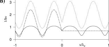
FIG. 1.: a) Experimental setup of an STM used to measure on a mesoscopic multiprobe conductor. The wire is biased with potentials $V_{1}$ and $V_{2}$, the applied potential at the tip is $V_{tip}$. This setup can be used to measure the average current or the fluctuation spectrum of the current flowing into the tip. b) Spatial variation of the current fluctuations and L(P)DOS of a ballistic wire with a $\delta$ barrier at $x=0$ with transmission probability $T=0.7$. The injectivity of the left contact, $\nu(x,1)$, (dashed line), and the LDOS $\nu(x)$, (dotted line) are in units of $1/hv$. The solid line gives the current fluctuation spectrum $\langle(\Delta I_{tip})^{2}\rangle$.

It is the purpose of this work to suggest and theoretically investigate experiments which use an STM to measure on multiprobe conductors as depicted in Fig. 1a). By applying different voltages at the contacts of the conductor one can drive a current through the sample already without the presence of a tunneling contact. Transport through multiprobe samples is characterized by a conductance matrix $G_{\alpha\beta}=(e^{2}/h)T_{\alpha\beta}$ describing the conductances between each two contacts $\alpha$ and $\beta$ of the sample. In the presence of a tunneling contact the overall conductance matrix of the sample plus tip now includes the conductances $G_{tip,\alpha}$ from a sample contact to the tip and the conductances $G_{\alpha,tip}$ from the tip to a sample contact. In contrast to the typical STM measurement which is characterized by one conductance only, we need for the arrangement of Fig. 1a) to determine two or more conductances. One aim of the present work is to investigate the densities which determine the transmission probabilities $T_{tip,\alpha}$ and $T_{tip,\alpha}$ for transmission from and to the tip. Once the conductance matrix is known we can use Büttiker’s formula[3] which expresses the current flowing into the contacts $\alpha$ of an arbitrary phase-coherent multiprobe conductor with the help of its scattering matrix and the Fermi distribution functions $f_{\alpha}(E)$ of the electrons in the reservoirs[3],

$$\langle I_{\alpha}\rangle=\frac{e}{h}\sum_{\beta}\int dET_{\alpha\beta}(E)\{f_{\alpha}(E)-f_{\beta}(E)\}\,.$$ (1)

Contacts weakly coupled to a multiprobe conductor have been investigated by Engquist and Anderson[4], using scattering matrices to describe the splitting of currents between conductor and tip. This discussion allowed a derivation of Landauer’s resistance formula[5] without appealing to screening arguments (local charge neutrality). Only currents but not their quantum mechanical amplitudes where considered in Ref. [4]. Subsequently, Imry[6] applied the Fermi Golden Rule to investigate this problem. A fully phase coherent discussion of a weak coupling contact (also using scattering matrices) was provided by one of us [7]. Here we return to this problem. Instead of using scattering matrices which describe the coupling of the tip to the sample and a separate scattering matrix for the sample, we start from the overall scattering matrix which includes all components of the system under investigation, the sample and the tip, and use a Green’s function technique to arrive at the results[8]. Such an approach permits readily to express results either in terms of scattering matrices or wave functions.

Average current — We find that the transmission probability from one contact $\alpha$ into the tip is no longer proportional to the total LDOS but only to a part of it, a local partial density of states (LPDOS) $\nu(x,\alpha)$[9, 10], called injectivity of the contact $\alpha$ at the coupling point $x$. The transmission from the tip into a contact $\alpha$ is proportional to another LPDOS $\nu(\alpha,x)$, called emissivity[9, 11] of the point $x$ into contact $\alpha$. We find[8]

$$T_{tip,\alpha}=4\pi^{2}\nu_{tip}|t|^{2}\nu(x,\alpha)\quad\mbox{and}\quad T_{\alpha,tip}=4\pi^{2}\nu(\alpha,x)|t|^{2}\nu_{tip}\,.$$ (2)

These results can be viewed as generalized Bardeen formulae for tunneling into multiprobe samples. The injectivity $\nu(x,\alpha)$ can be expressed with the help of the scattering states $\psi_{\alpha m}$ which represent an incoming electron from one of the open channels $m$ of contact $\alpha$ scattered in all channels of all contacts, $\nu(x,\alpha)=\sum_{m\in\alpha}(1/hv_{\alpha m})|\psi_{\alpha m}(x)|^{2}$. Here, $1/hv_{\alpha m}$ is the density of scattering states in channel $m$ of contact $\alpha$ and $v_{\alpha m}$ is their Fermi velocity. The injectivity of a contact $\alpha$ thus gives the density of states at the Fermi energy and at the position $x$ for charge carriers which entered the sample through contact $\alpha$. Injectivity and emissivity obey the sum rule $\sum_{\alpha}\nu(x,\alpha)=\sum_{\alpha}\nu(\alpha,x)=\nu(x)$ so that Eqs. (2) reduce to the well known Bardeen result in the case where the conductor is only connected to one single electron reservoir. Whereas the LDOS $\nu(x)$ is an even function of the magnetic field $B$, the injectivity and emissivity are related to each other by the symmetry relation $\nu_{B}(\alpha,x)=\nu_{-B}(x,\alpha)$. The emissivity can therefore be expressed with the help of the scattering states of the Hamilton operator in which the magnetic field has been reversed. In addition, this symmetry relation manifestly shows that the transmission probabilities, Eqs. (2), satisfy the Onsager-Casimir reciprocity relation[3], $T_{\alpha,tip}(B)=T_{tip,\alpha}(-B)$.

Using (2) in Eq. (1) we can express the current flowing into the tip in terms of the applied potentials and the injectivities of the sample. At finite temperature we have

$$\langle I_{tip}\rangle=\frac{e}{h}\int dET_{ts}(x)\{f_{tip}(E)-f_{eff}(x)\}$$ (3)

with the two-probe tip-to-sample transmission $T_{ts}(x)=4\pi^{2}\nu_{tip}|t|^{2}\nu(x)$ and the effective local distribution function

$$f_{eff}(x)=\sum_{\alpha}\frac{\nu(x,\alpha)}{\nu(x)}f_{\alpha}(E)\,.$$ (4)

This expression gives the local non-equilibrium distribution of charge carriers at the point $x$ inside the conductor. Its energy dependence comes from the Fermi distribution functions and a possible energy dependence of the L(P)DOS. Pothier et al.[12] measured an over a spatially wide range averaged non-equilibrium distribution function using a large superconducting tunneling contact on a diffusive wire. Eq. (3) has the form of the current in a two probe system, one probe being the tip, where the electron distribution is described by the Fermi function $f_{tip}(E)$ and an other probe where the electron distribution is given by the effective distribution function $f_{eff}(x)$. This effective distribution function does not account for any energy relaxation of the charge carriers inside the conductor. We assume that electron-electron and electron-phonon interactions can be neglected for the system under consideration and therefore the phase of the charge carriers is conserved. However, the distribution function does contain via the L(P)DOS the quantum mechanical phase coherence of the electron wavefunction throughout the system. Our effective distribution can be used to describe the quasi-particle distribution in phase-coherent diffusive conductors, if energy relaxation and dephasing can be neglected. To describe transport and noise in diffusive conductors one can also use the semiclassical Boltzmann-equation approach, which introduces a distribution function which does not contain the quantum-mechanical phase-coherence but where energy relaxation processes can be modeled quite easily. However, the distribution function of this semiclassical approach can not be used for conductors where phase-coherence is essential.

At zero temperature we can replace the Fermi functions in Eq. (3) by step functions and get in linear response to the applied potentials

$$\langle I_{tip}\rangle=G(x)\{V_{tip}-V_{eff}(x)\}\quad\mbox{with}\quad V_{eff}(x)=\sum_{\alpha}\frac{\nu(x,\alpha)}{\nu(x)}V_{\alpha}\,,$$ (5)

and the conductance $G(x)=(e^{2}/h)T_{ts}(x)$ has to be taken at the Fermi energy. A particularly interesting setup is, when the tip is used as a voltage probe, i. e. we demand that there is no net current flowing into the tip, $\langle I_{tip}\rangle=0$. Similar experiments, also called scanning tunneling potentiometry, have been reported in [13]. From Eq. (5) we find that at zero temperature the voltage one has to apply at the tip to achieve the zero-current condition is exactly the effective voltage $V_{eff}(x)$ defined in Eq. (5). The injectivities $\nu(x,\alpha)$ are determined by the equilibrium electrostatic potential $U(x)$ in the sample and, therefore, also the measured effective potential $V_{eff}(x)$ depends on the electrostatic potential. However, there is no direct relation between the measured potential and the actual electrostatic potential in the sample[9].

In the following we want to evaluate the effective distribution function or voltage for a metallic diffusive wire and for a wire with a barrier. First, we consider a diffusive wire of length $L$ to which two electron reservoirs are attached at the left end (x=0) and at the right end (x=L). The injectivity of the left contact (contact 1) and the right contact (contact 2) is then averaged over many different disorder configurations $\nu(x,1)=\nu_{0}(L-x)/L$ and $\nu(x,2)=\nu_{0}x/L$ with the constant LDOS $\nu_{0}$. This gives for the effective distribution function the known classical result $f_{eff}(x)=f_{1}(E)(L-x)/L+f_{2}(E)x/L$. It is interesting to contrast this result, with a a fully phase-coherent, sample specific result. We investigate the potential measured on a ballistic one-channel wire with a barrier at $x=0$ leading to the transmission probability $T$ and reflection probability $R=1-T$. Such a barrier generates strong, Friedel-like oscillations[7, 8] in the neighborhood of the barrier. To the left of the barrier, the injectivity of the left contact, contact 1, and right contact, contact 2, are

$$\nu(x,1)=\frac{1}{hv}(1+R+2\sqrt{R}\cos(2k_{F}x+\phi))\quad\mbox{and}\quad\nu(x,2)=\frac{1}{hv}T\,,$$ (6)

were $\phi$ is the phase acquired by reflected particles. At zero temperature this gives the oscillating effective voltage $V_{eff}(x)=V_{1}-T(V_{1}-V_{2})/\{2+2\sqrt{R}\cos(2k_{F}x+\phi)\}$. The voltages measured to the left and to the right of a scattering region can be used to find the four-probe resistance of the scattering region, which is defined as the measured potential drop divided by the current flowing through the scattering region[3]. The measured resistance will in general strongly depend on the exact positions where the voltage is measured as the strong oscillations in $V_{eff}(x)$ show.

Current fluctuations — Until now, we were only interested in the average currents given by Eq. (1). Now, we want to go one step further and investigate the fluctuations of the current away from its average value. The current fluctuation spectrum can give more information about the transport properties of a conductor than can be drawn from pure conductance measurements. Van den Brom and van Ruitenbeek[14] used combined conductance and current fluctuation measurements to characterize the detailed transport mechanism through few-atom gold contacts. Shot noise measurements have also been used to identify the fractional charge of the quasiparticles in the fractional quantum hall regime[15]. The low-frequency current fluctuation, respectively, correlation spectra are defined as the Fourier transform of the current-current correlator and given in terms of the scattering matrix ${\bf s}_{\alpha\beta}$ of the system as[16]

$$\langle\Delta I_{\alpha}\Delta I_{\beta}\rangle=\int dt\langle\Delta I_{\alpha}(t+t_{0})\Delta I_{\beta}(t_{0})\rangle=\frac{2e^{2}}{h}\sum_{\delta\gamma}\int dE{\rm Tr}[A_{\delta\gamma}(\alpha)A_{\gamma\delta}(\beta)]f_{\delta}(1-f_{\gamma})\,.$$ (7)

with $\Delta I_{\alpha}(t)=I_{\alpha}(t)-\langle I_{\alpha}(t)\rangle$ and the current matrix $A_{\beta\gamma}(\alpha)=\delta_{\alpha\beta}\delta_{\alpha\gamma}-{\bf s}_{\alpha\beta}^{\dagger}{\bf s}_{\alpha\gamma}$. If the two indices $\alpha$ and $\beta$ are equal, then this equation gives the current-fluctuation spectrum at the contact $\alpha$. Otherwise, the equation gives the correlation spectrum of the currents at contacts $\alpha$ and $\beta$. Current fluctuations at the contacts of a mesoscopic conductor have been measured by many groups[17]. Birk et al.[18] used an STM to measure the shot-noise on a tunneling contact. Correlations of currents at two different contacts of a sample have been measured only recently by Henny et al.[19] and Oliver et al.[20].

We calculate the current-fluctuation spectrum at the tunneling contact for the setup shown in Fig. 1a). As in our discussion of the sample to tip conductances, Eq. (2), we start with the scattering matrix of the entire system (wire and tip) and develop the scattering matrix elements describing scattering from and to the tip to the lowest order in the coupling energy $|t|$ of the tip. We assume that the potential at the tip is adjusted such that the average current at the tip vanishes. Then, using $G(x)=(e^{2}/h)4\pi^{2}\nu_{tip}|t|^{2}\nu(x)$, we find for the fluctuations of the current at the tip

$$\langle(\Delta I_{tip})^{2}\rangle=4\int dEG(x)\{1-f_{tip}(E)\}f_{eff}(x)\,.$$ (8)

We see, that the fluctuations are also determined by the effective distribution function, Eq. (4).

At elevated temperatures the fluctuations are due to thermal noise in addition with an excess noise, called shot-noise, which is due to the discreteness of the charge carriers. In Eq. (8) the integral over energy is from the bottom of the conduction band to infinity. At a temperature $T$ and applied potential differences $\Delta V$, the relevant contribution to the current fluctuations comes from the integration over an energy intervall of $\Delta E\approx\mbox{max}(e\Delta V,kT)$ around the Fermi energy. If the L(P)DOS are (nearly) independent of energy in this energy range, we can evaluate the integral over products of Fermi functions and get

$$\langle(\Delta I_{tip})^{2}\rangle=2eG(x)\Delta V\frac{\nu(x,1)}{\nu(x)}\frac{\nu(x,2)}{\nu(x)}\left\{\coth\left(\frac{\nu(x,1)}{\nu(x)}\frac{e\Delta V}{2kT}\right)+\coth\left(\frac{\nu(x,2)}{\nu(x)}\frac{e\Delta V}{2kT}\right)\right\}$$ (9)

with $\Delta V=V_{1}-V_{2}$ the applied potential at the wire. In the limit of high temperature, $kT\gg e\Delta V$, this equation leads to the Johnson-Nyquist formula for thermal noise, $\langle(\Delta I_{tip})^{2}\rangle=4eG(x)kT$. At zero-temperature, we are dealing with pure shot-noise. If we restrict ourselves to small potential differences so that linear response theory is justified, the fluctuation spectrum is completely determined by the properties of the system (its LPDOS) at the Fermi-energy[21],

$$\langle(\Delta I_{tip})^{2}\rangle=4eG(x)\Delta V\frac{\nu(x,1)}{\nu(x)}\left(1-\frac{\nu(x,1)}{\nu(x)}\right)\,.$$ (10)

Using the injectivities, Eq. (6), the measurement of the current fluctuation spectrum, Eq. (10), is illustrated in Fig. 1b) for the case of a measurement on a ballistic one channel conductor with a $\delta$-barrier at $x=0$ leading to the transmission probability $T=0.7$.

In conclusion, we presented generalized Bardeen formulae which for the transmission from the sample contacts to the tunneling tip are related to a local partial density of states, the injectivities $\nu(x,\alpha)$, and for the transmission from the tip to the sample contacts are related to the emissivities. We have shown that measurements of the average current and the fluctuations of the current at a tunneling tip which probes a phase-coherent multiprobe sample are determined by an effective local non-equilibrium distribution function. This distribution function is given as products of injectivities and the equilibrium Fermi distribution functions in the electron reservoirs. We illustrated the results for the case of ballistic conductors with barriers and metallic diffusive wires.

This work was supported by the Swiss National Science Foundation.

REFERENCES

- [1] Ph. Avouris, I.-W. Lyo, and Y. Hasegawa, IBM J. Res. Dev. 39, 603 (1995), and other articles in the same issue.
- [2] J. Tersoff and D. R. Hamann, Phys. Rev. B 31, 805 (1985); J. Bardeen, Phys. Rev. Lett. 6, 57 (1961).
- [3] M. Büttiker, Phys. Rev. Lett. 57, 1761 (1986); IBM J. Res. Dev. 32, 317 (1988).
- [4] H.-L. Engquist and P. W. Anderson, Phys. Rev. B 24, 1151 (1981).
- [5] R. Landauer, Phil. Mag. 21, 863 (1970); IBM J. Res. Develop. 1, 223 (1957).
- [6] Y. Imry, in Directions in Condensed Matter Physics, edited by G. Grinstein and G. Mazenko, (World Scientific Singapore, 1986). p. 101.; see also O. Entin-Wohlmann, C. Hartzstein, and Y. Imry, Phys. Rev. B 34, 921 (1986).
- [7] M. Büttiker, Phys. Rev. B 40, 3409 (1989).
- [8] T. Gramespacher and M. Büttiker, Phys. Rev. B 56, 13026 (1997).
- [9] M. Büttiker, J. Phys. Condens. Matter 5, 9361 (1993).
- [10] M. Büttiker and T. Christen, in: Quantum Transport in Semiconductor Submicron Structures, Ed. by B. Kramer, NATO ASI Series, Vol. 326 (Kluwer, Dordrecht, 1996), p. 263.
- [11] I. B. Levinson, Sov. Phys. JETP 68, 1257 (1989).
- [12] H. Pothier et al., Phys. Rev. Lett. 79, 3490 (1997).
- [13] P. Muralt et al., Appl. Phys. Lett. 50, 1352 (1987); J. R. Kirtley, S. Washburn, and M. J. Brady, Phys. Rev. Lett. 60, 1546 (1988); B. G. Briner et al., Phys. Rev. B 54, R5283 (1996).
- [14] H. E. van den Brom and J. M. van Ruitenbeek, cond-mat/9810276.
- [15] L. Saminadayar, D. C. Glattli, Y. Jin, and B. Etienne, Phys. Rev. Lett. 79, 2526 (1997); R. de-Picciotto et al., Nature 389, 162 (1997).
- [16] M. Büttiker, Phys. Rev. Lett. 68, 843 (1992); Phys. Rev. B 46, 12485 (1992).
- [17] M. Reznikov et al., Phys. Rev. Lett. 75, 3340 (1995); A. Kumar et al., ibid. 76, 2778 (1996); R. J. Schoelkopf et al., ibid. 78, 3370 (1997).
- [18] H. Birk, M. J. M. de Jong, and C. Schönenberger, Phys. Rev. Lett. 75, 1610 (1995).
- [19] M. Henny, S. Oberholzer, C. Strunk, and C. Schönenberger, (unpublished); M. Henny, Thesis (University of Basel, 1998).
- [20] W. D. Oliver, J. Kim, R. C. Liu, and Y. Yamamoto, (unpublished).
- [21] T. Gramespacher and M. Büttiker, Phys. Rev. Lett. 81, 2763 (1998).