Autocorrelations from the transfer matrix DMRG method

Abstract

Extending the transfer matrix DMRG algorithm, we are able to calculate imaginary time spin autocorrelations with high accuracy (absolute error $<10^{-6}$) over a wide temperature range ($0<\beta J<20$). After analytic continuation using the rules of probability theory along with the entropic prior (MaxEnt), we obtain real frequency spectra for the XY model, the isotropic Heisenberg and the gaped Heisenberg-Ising model. Available exact results in some limits allow for a critical evaluation of the quality of answers expected from this procedure. We find that high precision data are still insufficient for resolving specific lineshapes such as low frequency divergences. However, the method is appropriate for identifying low temperature gaps and peak positions.

I Introduction

Finite temperature dynamic correlations are the link between experiment and theory. In spite of their relevance, it seems that for strongly interacting electronic or magnetic systems, no reliable, direct theoretical methods exist for their evaluation. This absence is particularly felt recently in the field of quasi one-dimensional magnetic materials, where excellent samples, detailed neutron scattering and NMR experiments[1, 2] call for a better understanding of dynamic form factors. In this context, numerical simulation techniques can provide valuable information. However, these are also subject to rather severe limitations. On the one hand, real time methods based on the exact diagonalization of the Hamiltonian matrix have been restricted to small systems. As a consequence, the extrapolation to the thermodynamic limit is often unreliable, especially in the low temperature regime.[3] Related methods such as the moment expansion or the recursion method[4] can provide reliable short time correlations, however, the extrapolation to long times is left uncertain. Until now, real time methods have been insufficient for discussing low frequency properties, for instance, they cannot decide about diffusive or ballistic transport. [5, 6, 7]

On the other hand, imaginary time methods such as quantum Monte Carlo [8] (QMC) have to face the ill-conditioned analytical continuation problem. In this context, it is reasonable to expect that the higher accuracy of the transfer matrix DMRG calculations,[9, 10] free of stochastic errors, might help. This method has been applied successfully to several interesting (quasi-)one dimensional systems. [11, 12, 13, 14, 15, 16, 17, 18, 19] In this work we describe in detail an extension of the transfer matrix DMRG method proposed in Ref.[10] to calculate imaginary time correlations.[20] We show that these can be very accurately determined, especially for local correlations. In addition, we present an extended critical discussion on the potential of this method to obtain reliable real frequency spectra. Of course, the transfer matrix DMRG method is limited to quasi-one dimensional systems.

In order to investigate whether the combination of transfer matrix DMRG and analytical continuation methods can provide accurate dynamic correlations, we focus on the $s=1/2$ antiferromagnetic Heisenberg Hamiltonian:

$$H=J\sum_{l}(S_{l}^{x}S_{l+1}^{x}+S_{l}^{y}S_{l+1}^{y}+\Delta S_{l}^{z}S_{l+1}^{z}),$$ (1)

where $S_{l}^{\alpha}=\frac{1}{2}\sigma_{l}^{\alpha}$, $\sigma_{l}^{\alpha}$ are the Pauli spin operators with components $\alpha=x,y,z$ at site $l$. In the following we will take $J$ as the unit of energy.

This model represents a good playground for tests since in the XY limit ($\Delta=0$) exact results at all temperatures for the longitudinal zz-correlation and at $T=0,\infty$ for the transverse xx-correlation are known. For $\Delta=1$, and $\Delta\geq 1$ where the spectrum is gaped, the two spinon contribution to the transverse correlation at $T=0$ was recently exactly evaluated.[21, 22]

The paper is organized as follows: section II explains how to extend the transfer matrix DMRG technique for obtaining imaginary time correlations and also provides a summary of the analytical continuation methods. In III A and III B, we look closely at the XY model and compare our results to exact solutions. Among various analytical continuation procedures, we find the MaxEnt method to be the most reliable. The results for the isotropic point ($\Delta=1$) are presented in section III C and those for the gaped regime ($\Delta=2,4$) in section III D.

II Technique

A Notation

Before explaining the transfer matrix DMRG technique, let us first fix some notation. The basic quantity from which the nuclear spin relaxation rate $1/T_{1}$ and the neutron scattering cross section can be determined is the dynamical structure factor

$$S^{\alpha}_{ij}(\omega)=\int_{-\infty}^{+\infty}e^{i\omega t}\langle S^{\alpha}_{i}(t)S^{\alpha}_{j}(0)\rangle dt$$ (2)

where $\alpha=z$ for the longitudinal and $\alpha=x$ for the transverse correlations. $S^{\alpha}_{i}(t)=e^{itH}S^{\alpha}_{i}e^{-itH}$ and the average $\langle\bullet\rangle$ is taken in the canonical ensemble at the inverse temperature $\beta=1/T$. $S^{\alpha}_{ij}(\omega)$ is a positive function and the autocorrelations $i=j$ satisfy the sum-rule

$$\frac{1}{2\pi}\int_{-\infty}^{+\infty}S^{\alpha}_{ii}(\omega)d\omega=\frac{1}{4}$$ (3)

at all temperatures. Using the transfer matrix DMRG method we will study the imaginary time Green’s function

$$G^{\alpha}_{ij}(\tau)=\langle S^{\alpha}_{i}(\tau)S^{\alpha}_{j}\rangle$$ (4)

where $S^{\alpha}_{i}(\tau)=e^{\tau H}S^{\alpha}_{i}e^{-\tau H}$.

It is related to the real frequency correlations through the linear integral equation:

$$G^{\alpha}_{ij}(\tau)=\frac{1}{2\pi}\int_{0}^{\infty}K(\tau,\omega)S^{\alpha}_{ij}(\omega)d\omega$$ (5)

$$K(\tau,\omega)=e^{-\tau\omega}+e^{-(\beta-\tau)\omega}$$ (6)

where the detailed balance condition $S^{\alpha}_{ij}(-\omega)=e^{-\beta\omega}S^{\alpha}_{ij}(\omega)$ has been included in the kernel $K(\tau,\omega)$. Notice also that using the symmetry $K(\tau,\omega)=K(\beta-\tau,\omega)$ it is only necessary to calculate $G^{\alpha}_{ij}(\tau)$ in the interval $[0,\beta/2]$. The decomposition of the integrand in Eq. (5) into $K(\tau,\omega)$ and $S^{\alpha}_{ij}(\omega)$ is not unique. In fact, it is sometimes better (see the xx correlations in the XY model) to reconstruct the symmetric correlation function ${\tilde{S}}^{\alpha}_{ij}(\omega)$, even in $\omega$, corresponding to the Fourier transform of the anti- commutator correlations. For this purpose, we rewrite Eq. (5) as

$$G^{\alpha}_{ij}(\tau)=\frac{1}{2\pi}\int_{0}^{\infty}{\tilde{K}}(\tau,\omega){\tilde{S}}^{\alpha}_{ij}(\omega)d\omega$$ (7)

with

$${\tilde{K}}(\tau,\omega)=K(\tau,\omega)/(1+e^{-\beta\omega}),$$ (8)

$${\tilde{S}}^{\alpha}_{ij}(\omega)=S^{\alpha}_{ij}(\omega)(1+e^{-\beta\omega}).$$ (9)

This scheme will be referred to as the symmetric scheme.

B Transfer matrix DMRG

In this purely technical part, we will explain in detail how one can calculate imaginary time correlations by extending the transfer matrix DMRG method developed in reference[[10]].

1 Thermodynamics

Let us briefly recall how the transfer matrix representation of the partition function is used to calculate thermodynamic quantities. First, we split the Hamiltonian (1) into odd and even bond terms:

$$H=H_{o}+H_{e}$$ (10)

$$H_{o}=h_{1}+h_{3}+h_{5}+\cdots$$ (11)

$$H_{e}=h_{2}+h_{4}+h_{6}+\cdots$$ (12)

$$h_{i}=S_{i}^{x}S_{i+1}^{x}+S_{i}^{y}S_{i+1}^{y}+\Delta S_{i}^{z}S_{i+1}^{z},$$ (13)

so that the all even (respectively odd) terms $h_{i}$ commute with each other. Then, using the Trotter-Suzuki decomposition and doing the standard insertion of the identity $1=\prod_{i=1}^{N}\sum_{\{s_{k^{\prime}}^{i}\}}|s_{k^{\prime}}^{i}\rangle\langle s_{k^{\prime}}^{i}|$ at each inverse temperature slice $k^{\prime}=1,2,\ldots,2M$, we can express the partition function in terms of the quantum transfer matrix ${\cal T}_{M}$: [23, 24]

$$Z={\rm Tr}\,e^{-\beta H}={\rm Tr}\left[e^{-\epsilon H_{o}}e^{-\epsilon H_{e}}\right]^{M}+{\cal O}(\epsilon^{2})\,,$$ (14)

$${\rm Tr}\left[e^{-\epsilon H_{o}}e^{-\epsilon H_{e}}\right]^{M}={\rm Tr}\,\left[{\cal T}_{M}\right]^{N/2}.$$ (15)

Here $M$ is the Trotter number, $\epsilon=\beta/M$ and $\beta=1/T$. In the last step of Eq.(15), the summation indices have been permuted so that the space and Trotter (inverse temperature) directions are interchanged. ${\cal T}_{M}$ is a non-symmetric matrix given by the product of $2M$ local transfer matrices

$$\langle\sigma^{1}_{1}\cdots\sigma^{1}_{2M}|{\cal T}_{M}|\sigma_{1}^{3}\cdots\sigma^{3}_{2M}\rangle=\sum_{\{\sigma^{2}_{k}\}}\prod_{k=1}^{M}\tau(\sigma^{1}_{2k-1}\sigma^{1}_{2k}|\sigma^{2}_{2k-1}\sigma^{2}_{2k})\tau(\sigma^{2}_{2k}\sigma^{2}_{2k+1}|\sigma^{3}_{2k}\sigma^{3}_{2k+1})$$ (16)

with periodic boundary condition in the Trotter direction ($\sigma_{2M+1}=\sigma_{1}$), $\sigma^{i}_{k}=(-1)^{i+k}s^{i}_{k}$ and

$$\tau(\sigma^{i}_{k}\sigma^{i}_{k+1}|\sigma^{i+1}_{k}\sigma^{i+1}_{k+1})=\langle s^{i+1}_{k+1},s^{i}_{k+1}|\exp(-\epsilon\hat{h}_{i})|s^{i}_{k},s^{i+1}_{k}\rangle.$$ (17)

The real space indices are denoted by $i$, the Trotter direction by $k$ and $S_{i}^{z}|s^{i}_{k}\rangle=s^{i}_{k}|s^{i}_{k}\rangle$. The sign in the definition of $\sigma^{i}_{k}$ is chosen such that $\tau$ conserves $\sigma$: $\sigma^{i}_{k}+\sigma^{i}_{k+1}=\sigma^{i+1}_{k}+\sigma^{i+1}_{k+1}$. Eqs. (15)-(17) are best represented as a 2-dimensional checkerboard shown in Fig. 1(a). The arrow in the left corner emphasizes that $\tau$ propagates in the real space direction. Fig. 1(b) shows how the full checkerboard is cut along the real space direction in $N/2$ identical quantum transfer matrices ${\cal T}_{M}$.

In the limit $N\rightarrow\infty$, the partition function $Z$ is given by the maximum eigenvalue $\lambda_{\rm max}^{N/2}$. Thermodynamic quantities such as the magnetization or the internal energy can be obtained from the corresponding left $\left<\psi^{L}\right|$ and right $\left|\psi^{R}\right>$ eigenvectors of the transfer matrix ${\cal T}_{M}$.[10]

Let us emphasize that the method provides results free of finite size errors, the thermodynamic limit being obtained automatically, due to the exponent $N/2$ in Eq. (15). Remaining errors are the systematic ${\cal O}(\epsilon^{2})$ Trotter error and the systematic error introduced by the truncation of the basis set for the density matrix.[25]

2 Imaginary time correlation function

We now turn to the imaginary time correlation function (4) and restrict ourselves to $G_{ij}^{z}(\tau)$, the extension to $G_{ij}^{x}(\tau)$ being straightforward. For convenience, we express (4) as

$$G_{ij}^{z}(\tau) = \frac{{\cal N}_{ij}(\tau)}{Z}$$ (18)

$${\cal N}_{ij}(\tau) = {\rm Tr}\left(S_{i}^{z}e^{-\tau H}S_{j}^{z}e^{-(\beta-\tau)H}\right)={\rm Tr}\left(S_{i}^{z}(e^{-\epsilon H})^{k}S_{j}^{z}(e^{-\epsilon H})^{M-k}\right),$$ (19)

where $\tau=\epsilon k$ and $k=0,1,\ldots,M-1$. Using the following symmetric decomposition:

$$e^{-\epsilon H}=e^{-\frac{\epsilon}{2}H_{o}}e^{-\epsilon H_{e}}e^{-\frac{\epsilon}{2}H_{o}}+{\cal O}(\epsilon^{2}),$$ (20)

we have

$${\cal N}_{ij}(\tau) ={\rm Tr} \,(\,\underbrace{e^{-\frac{\epsilon}{2}H_{o}}S_{i}^{z}e^{-\frac{\epsilon}{2}H_{o}}e^{-\epsilon H_{e}}}_{1}\underbrace{e^{-\epsilon H_{o}}e^{-\epsilon H_{e}}}_{2}\cdots\underbrace{e^{-\epsilon H_{o}}e^{-\epsilon H_{e}}}_{k}$$ (22)

$$\underbrace{e^{-\frac{\epsilon}{2}H_{o}}S_{j}^{z}e^{-\frac{\epsilon}{2}H_{o}}e^{-\epsilon H_{e}}}_{k+1}\underbrace{e^{-\epsilon H_{o}}e^{-\epsilon H_{e}}}_{k+2}\cdots\underbrace{e^{-\epsilon H_{o}}e^{-\epsilon H_{e}}}_{M}\,)\,.$$

up to ${\cal O}(\epsilon^{2})$ corrections.

As for the partition function, we insert identities along the horizontal Trotter slices, permute the summation indices in the trace and form local transfer matrix chains along the Trotter direction to obtain an expression similar to Eq.(15):

$${\cal N}_{ij}(\tau)={\rm Tr}[{\cal T}_{M}^{ij}(k)~{}({\cal T}_{M})^{(\frac{N}{2}-\left[\frac{j}{2}\right]+\left[\frac{i}{2}\right]-1)}].$$ (23)

Here $[\frac{i}{2}]$ is the closest integer larger than or equal to $\frac{i}{2}$. In defining ${\cal T}_{M}^{ij}(k)$, we have to differentiate the case $j=i,i+1$ from $j>i+1$. First, however, we need to define the local spin transfer matrices

$$\tau^{z}_{l}(\sigma^{i}_{k},\sigma^{i}_{k+1}|\sigma^{i+1}_{k},\sigma^{i+1}_{k+1})=\langle s_{k}^{i},s_{k}^{i+1}|{\rm e}^{-\frac{\epsilon}{2}h_{i}}S_{l}^{z}{\rm e}^{-\frac{\epsilon}{2}h_{i}}|s_{k+1}^{i},s_{k+1}^{i+1}\rangle$$ (24)

$$\tau^{z}_{lm}(\sigma^{i}_{k},\sigma^{i}_{k+1}|\sigma^{i+1}_{k},\sigma^{i+1}_{k+1})=\langle s_{k}^{i},s_{k}^{i+1}|{\rm e}^{-\frac{\epsilon}{2}h_{i}}S_{l}^{z}S_{m}^{z}{\rm e}^{-\frac{\epsilon}{2}h_{i}}|s_{k+1}^{i},s_{k+1}^{i+1}\rangle$$ (25)

where $l,m=i,i+1$. Then, for $j>i+1$,

$${\cal T}_{M}^{ij}(k)={\cal T}_{M}^{i}(0)~{}({\cal T}_{M})^{\left[\frac{j}{2}\right]-\left[\frac{i}{2}\right]-1}~{}{\cal T}_{M}^{j}(k)$$ (26)

with

$$\langle\sigma^{i}_{1}\cdots\sigma^{i}_{2M}|{\cal T}^{l}_{M}(k)|\sigma_{1}^{i+2}\cdots\sigma^{i+2}_{2M}\rangle$$ (27)

$$= \sum_{\{\sigma^{i+1}_{n}\}}\tau_{l}(\sigma^{i}_{2k+1},\sigma^{i}_{2k+2}|\sigma^{i+1}_{2k+1},\sigma^{i+1}_{2k+2})\tau(\sigma^{i+1}_{2k+2},\sigma^{i+1}_{2k+3}|\sigma^{i+2}_{2k+2},\sigma^{i+2}_{2k+3})$$ (28)

$$\times \prod_{k^{\prime}\in[1,M]}^{k^{\prime}\neq k+1}\tau(\sigma^{i}_{2k^{\prime}-1},\sigma^{i}_{2k^{\prime}}|\sigma^{i+1}_{2k^{\prime}-1},\sigma^{i+1}_{2k^{\prime}})\tau(\sigma^{i+1}_{2k^{\prime}},\sigma^{i+1}_{2k^{\prime}+1}|\sigma^{i+2}_{2k^{\prime}},\sigma^{i+2}_{2k^{\prime}+1}).$$ (29)

Again, these formulas can be nicely understood graphically as in Figs. 1(c) and 1(d), corresponding to Eqs. (23)-(27) for the case $N=6$, $M=3$ ,$i=1$ and $j=3,4$. In this case, the two local spin transfer matrices sit on different transfer matrix chains.

On the contrary, for $j=i,i+1$, they belong to the same chain:

$$\langle\sigma^{i}_{1}\cdots\sigma^{i}_{2M}|{\cal T}_{M}^{ij}(k)|\sigma_{1}^{i+2}\cdots\sigma^{i+2}_{2M}\rangle$$ (30)

$$= \sum_{\{\sigma^{i+1}_{n}\}}\tau^{z}_{l}(\sigma^{i}_{1},\sigma^{i}_{2}|\sigma^{i+1}_{1},\sigma^{i+1}_{2})\tau(\sigma^{i+1}_{2},\sigma^{i+1}_{3}|\sigma^{i+2}_{2},\sigma^{i+2}_{3})$$ (31)

$$\times \tau^{z}_{m}(\sigma^{i}_{2k+1},\sigma^{i}_{2k+2}|\sigma^{i+1}_{2k+1},\sigma^{i+1}_{2k+2})\tau(\sigma^{i+1}_{2k+2},\sigma^{i+1}_{2k+3}|\sigma^{i+2}_{2k+2},\sigma^{i+2}_{2k+3})$$ (32)

$$\times \prod_{k^{\prime}\in[1,M]}^{k^{\prime}\neq 1,k+1}\tau(\sigma^{i}_{2k^{\prime}-1},\sigma^{i}_{2k^{\prime}}|\sigma^{i+1}_{2k^{\prime}-1},\sigma^{i+1}_{2k^{\prime}})\tau(\sigma^{i+1}_{2k^{\prime}},\sigma^{i+1}_{2k^{\prime}+1}|\sigma^{i+2}_{2k^{\prime}},\sigma^{i+2}_{2k^{\prime}+1})$$ (33)

when $k=1,2,\ldots,M-1$ and

$$\langle\sigma^{i}_{1}\cdots\sigma^{i}_{2M}|{\cal T}_{M}^{ij}(k)|\sigma_{1}^{i+2}\cdots\sigma^{i+2}_{2M}\rangle$$ (34)

$$= \sum_{\{\sigma^{i+1}_{n}\}}\tau^{z}_{lm}(\sigma^{i}_{1},\sigma^{i}_{2}|\sigma^{i+1}_{1},\sigma^{i+1}_{2})\tau(\sigma^{i+1}_{2},\sigma^{i+1}_{3}|\sigma^{i+2}_{2},\sigma^{i+2}_{3})$$ (35)

$$\times \prod_{k^{\prime}\in[1,M]}^{k^{\prime}\neq 1}\tau(\sigma^{i}_{2k^{\prime}-1},\sigma^{i}_{2k^{\prime}}|\sigma^{i+1}_{2k^{\prime}-1},\sigma^{i+1}_{2k^{\prime}})\tau(\sigma^{i+1}_{2k^{\prime}},\sigma^{i+1}_{2k^{\prime}+1}|\sigma^{i+2}_{2k^{\prime}},\sigma^{i+2}_{2k^{\prime}+1}),$$ (36)

for $k=0$, corresponding to a static correlation.

Finally, we obtain for the imaginary time correlation

$$G_{ij}^{z}(\tau)=\frac{{\rm Tr}[{\cal T}_{M}^{ij}(k)~{}({\cal T}_{M})^{(\frac{N}{2}-\left[\frac{j}{2}\right]+\left[\frac{i}{2}\right]-1)}]}{{\rm Tr}({\cal T}_{M})^{\frac{N}{2}}}$$ (37)

In the limits $N\rightarrow\infty$ and $|i-j|\ll N$, this reduces to

$$G_{ij}^{z}(\tau)=\frac{\langle\psi^{L}|{\cal T}_{M}^{ij}(k)|\psi^{R}\rangle}{\lambda_{\rm max}^{\left[\frac{j}{2}\right]-\left[\frac{i}{2}\right]+1}}.$$ (38)

For systems with finite correlation length $\xi$, $G^{z}_{ij}(\tau)\sim\left<S^{z}_{i}\right>\left<S^{z}_{j}\right>$ when $|j-i|\gg\xi$, which can be verified systematically as $\xi$ is determined from $\xi^{-1}=\frac{1}{2}\ln\left|\frac{\lambda_{n}}{\lambda_{\rm max}}\right|$. $\lambda_{n}$ is the next largest eigenvalue of ${\cal T}_{M}$.

3 Renormalization of transfer matrices

Now that we have defined the relevant transfer matrices, we must explain how to construct them in practise. The purpose is to add successively new $\tau$ plaquettes to grow ${\cal T}_{M}$ in the Trotter direction (in the same spirit real sites are added to the Hamiltonian in the standard $T=0$ DMRG algorithm[25]) and simultaneously find a renormalization procedure that keeps the dimension of the matrix ${\cal T}_{M}$ fixed as the temperature is lowered. For this purpose, we cut ${\cal T}_{M}$ schematically in two halves as shown in Fig. 2 for the two generic cases of $M$ odd (a) and even (b). In the DMRG language, ${\cal T}_{M}$ is called the superblock, the right inner block (dashed line in Fig.2) plus the left edge $(\sigma_{1},\sigma_{1}^{{}^{\prime\prime}})$ the system and the left inner block plus the right edge $(\sigma_{2},\sigma_{2}^{{}^{\prime\prime}})$ the environment. We use $n_{s}$ and $n_{e}$ to label the basis sets in the inner of the system and environment blocks, respectively. The states at the left and right edges are labelled by $\sigma_{1}$ and $\sigma_{2}$. With this notation, we denote the elements of the right transfer matrix by ${\cal S}_{o}(\sigma_{1}^{\prime\prime},n_{s}^{\prime},\sigma_{2}^{\prime\prime};\sigma_{1},n_{s},\sigma_{2})$ or ${\cal S}_{e}(\sigma_{1}^{\prime},n_{s}^{\prime},\sigma_{2}^{\prime\prime};\sigma_{1}^{\prime\prime},n_{s},\sigma_{2})$ depending on whether the system consist of an even ($e$) or odd ($o$) number of $\tau$ plaquettes. When adding a new plaquette, the elements of the new system are given by the following recursion relation:

$${\cal S}_{e}(\sigma_{1}^{\prime},\tilde{n}_{s}^{\prime},\sigma_{2}^{\prime\prime};\sigma_{1}^{\prime\prime},\tilde{n}_{s},\sigma_{2})=\sum_{\sigma^{\prime\prime}}\tau(\sigma_{1}^{\prime},\sigma^{\prime}|\sigma_{1}^{\prime\prime},\sigma^{\prime\prime}){\cal S}_{o}(\sigma^{\prime\prime},n_{s}^{\prime},\sigma_{2}^{\prime\prime};\sigma,n_{s},\sigma_{2}),$$ (39)

$${\cal S}_{o}(\sigma_{1}^{\prime\prime},\tilde{n}_{s}^{\prime},\sigma_{2}^{\prime\prime};\sigma_{1},\tilde{n}_{s},\sigma_{2})=\sum_{\sigma^{\prime\prime}}\tau(\sigma_{1}^{\prime\prime},\sigma^{\prime\prime}|\sigma_{1},\sigma){\cal S}_{e}(\sigma^{\prime},n_{s}^{\prime},\sigma_{2}^{\prime\prime};\sigma^{\prime\prime},n_{s},\sigma_{2}),$$ (40)

where $\{\left|\tilde{n}_{s}\right>\}=\{\left|\sigma\right>\}\otimes\{\left|n_{s}\right>\}$. Initially, when $M=2$, ${\cal S}_{e}(\sigma_{1}^{\prime},\sigma^{\prime},\sigma_{2}^{\prime\prime};\sigma_{1}^{\prime\prime},\sigma,\sigma_{2})=\sum_{\sigma^{\prime\prime}}\tau(\sigma_{1}^{\prime},\sigma^{\prime}|\sigma_{1}^{\prime\prime},\sigma^{\prime\prime})\tau(\sigma^{\prime\prime},\sigma_{2}^{\prime\prime}|\sigma,\sigma_{2})$.

Similarly, the elements of the left transfer matrix ${\cal E}_{o}(\sigma_{1}^{\prime},n_{e}^{\prime},\sigma_{2}^{\prime};\sigma_{1}^{\prime\prime},n_{e},\sigma_{2}^{\prime\prime})$ or ${\cal E}_{e}(\sigma_{1}^{\prime\prime},n_{e}^{\prime},\sigma_{2}^{\prime};\sigma_{1},n_{e},\sigma_{2}^{\prime\prime})$, are given by

$${\cal E}_{e}(\sigma_{1}^{\prime\prime},\tilde{n}_{e}^{\prime},\sigma_{2}^{\prime};\sigma_{1},\tilde{n}_{e},\sigma_{2}^{\prime\prime})=\sum_{\sigma^{\prime\prime}}\tau(\sigma_{1}^{\prime\prime},\sigma^{\prime\prime}|\sigma_{1},\sigma){\cal E}_{o}(\sigma^{\prime},n_{e}^{\prime},\sigma_{2}^{\prime};\sigma^{\prime\prime},n_{e},\sigma_{2}^{\prime\prime}),$$ (41)

$${\cal E}_{o}(\sigma_{1}^{\prime},\tilde{n}_{e}^{\prime},\sigma_{2}^{\prime};\sigma_{1}^{\prime\prime},\tilde{n}_{e},\sigma_{2}^{\prime\prime})=\sum_{\sigma^{\prime\prime}}\tau(\sigma_{1}^{\prime},\sigma^{\prime}|\sigma_{1}^{\prime\prime},\sigma^{\prime\prime}){\cal E}_{e}(\sigma^{\prime\prime},n_{e}^{\prime},\sigma_{2}^{\prime};\sigma,n_{e},\sigma_{2}^{\prime\prime})$$ (42)

after one plaquette has been added, $\{\left|\tilde{n}_{e}\right>\}=\{\left|\sigma\right>\}\otimes\{\left|n_{e}\right>\}$.

When the number of states in $\{\left|\tilde{n}_{s}\right>\}$ ($\{\left|\tilde{n}_{e}\right>\}$) exceeds a given number $m$, the transfer matrices ${\cal S}_{e,o}$ (${\cal E}_{e,o}$) are renormalized by:

$${\cal A}_{e}(\sigma_{1}^{\prime},n_{s}^{\prime},\sigma_{2}^{\prime\prime};\sigma_{1}^{\prime\prime},n_{s},\sigma_{2})=\sum_{\tilde{n}_{s}^{\prime}\tilde{n}_{s}}O_{\cal A}^{l}(n_{s}^{\prime},\tilde{n}_{s}^{\prime}){\cal A}_{e}(\sigma_{1}^{\prime},\tilde{n}_{s}^{\prime},\sigma_{2}^{\prime\prime};\sigma_{1}^{\prime\prime},\tilde{n}_{s},\sigma_{2})O_{\cal A}^{r}(\tilde{n}_{s},n_{s}),$$ (43)

$${\cal A}_{o}(\sigma_{1}^{\prime\prime},n_{s}^{\prime},\sigma_{2}^{\prime\prime};\sigma_{1},n_{s},\sigma_{2})=\sum_{\tilde{n}_{s}^{\prime}\tilde{n}_{s}}O_{\cal A}^{l}(n_{s}^{\prime},\tilde{n}_{s}^{\prime}){\cal A}_{o}(\sigma_{1}^{\prime\prime},\tilde{n}_{s}^{\prime},\sigma_{2}^{\prime\prime};\sigma_{1},\tilde{n}_{s},\sigma_{2})O_{\cal A}^{r}(\tilde{n}_{s},n_{s}),$$ (44)

${\cal A}={\cal S}$ for the system block or ${\cal E}$ for the environment block, $n_{s}^{\prime},n_{s}=1,2,\ldots,m$. The transformation matrices $O^{l}_{\cal A}$ and $O^{r}_{\cal A}$ are constructed from the $m$ largest eigenvectors of the corresponding reduced, non-symmetric density matrices given in terms of the left and right eigenvectors of ${\cal T}_{M}$ by:

$$\rho_{s}={\rm Tr}_{n_{e},\sigma_{2}}|\psi^{R}\rangle\langle\psi^{L}|,~{}~{}~{}\rho_{e}={\rm Tr}_{n_{s},\sigma_{1}}|\psi^{R}\rangle\langle\psi^{L}|,$$ (45)

for the system and the environment. In terms of ${\cal S}$ and ${\cal E}$, the renormalized transfer matrix ${\cal T}_{M}$ corresponding to the superblock (Fig. 2) is given by

$${\cal T}_{M}(n_{e}^{\prime},\sigma_{2}^{\prime},\sigma_{1}^{\prime},n_{s}^{\prime};n_{e},\sigma_{2},\sigma_{1},n_{s})=\left\{\begin{array}[]{rl}\displaystyle{\sum_{\sigma_{1}^{\prime\prime},\sigma_{2}^{\prime\prime}}}&{\cal E}_{o}(\sigma_{1}^{\prime},n_{e}^{\prime},\sigma_{2}^{\prime};\sigma_{1}^{\prime\prime},n_{e},\sigma_{2}^{\prime\prime})\\ \times&{\cal S}_{o}(\sigma_{1}^{\prime\prime},n_{s}^{\prime},\sigma_{2}^{\prime\prime};\sigma_{1},n_{s},\sigma_{2}),\\ \displaystyle{\sum_{\sigma_{1}^{\prime\prime},\sigma_{2}^{\prime\prime}}}&{\cal E}_{e}(\sigma_{2}^{\prime\prime},n_{e}^{\prime},\sigma_{2}^{\prime};\sigma_{1},n_{e},\sigma_{2}^{\prime\prime})\\ \times&{\cal S}_{e}(\sigma_{1}^{\prime},n_{s}^{\prime},\sigma_{2}^{\prime\prime};\sigma_{1}^{\prime\prime},n_{s},\sigma_{2})\end{array}\right.$$ (50)

for $M/2$ odd or even.

Many systems of interest have spatial reflection symmetry. For these, we can obtain the left transfer matrix from transposition of the right one so that for instance, ${\cal E}_{o}(\sigma_{1}^{\prime},n_{e}^{\prime},\sigma_{2}^{\prime};\sigma_{1}^{\prime\prime},n_{e},\sigma_{2}^{\prime\prime})={\cal S}_{o}(\sigma_{1}^{\prime\prime},n_{e},\sigma_{2}^{\prime\prime};\sigma_{1},n_{e}^{\prime},\sigma_{2})$. Consequently, the left eigenvector of $\langle\psi^{L}|$ can be obtained from $|\psi^{R}\rangle$: $\psi^{L}(n_{s},\sigma_{2},\sigma_{1},n_{e})=\psi^{R}(n_{e},\sigma_{2},\sigma_{1},n_{s})$. For systems without reflection symmetry such as zigzag or dimerized chains, left and right transfer matrices and eigenvectors must be evaluated separately.

As a last technical step, we have to explain how to renormalize ${\cal T}_{M}^{ij}(k)$, needed for evaluating $G^{z}_{ij}(\tau)$. Again, we must distinguish two cases:

For $j=i,i+1$, the two local spin transfer matrices are located on the same transfer matrix chain. In this case, we can separate ${\cal T}_{M}^{ij}(k)$ into left ${\cal E}_{e,o}^{j}(k)$ and right ${\cal S}_{e,o}^{i}$ parts, similar to what we did for ${\cal T}_{M}$. As $G^{z}_{ij}(\tau)=G^{z}_{ij}(\beta-\tau)$, it is sufficient if $k=0,1,\ldots,M/2$ so that there is always exactly one local spin transfer matrix in each half of ${\cal T}_{M}^{ij}(k)$ (Fig. 3.) The blocks ${\cal E}_{e,o}^{j}(k)$ and ${\cal S}_{e,o}^{i}$ are renormalized according to Eqs. (40)-(44) except that $\tau$ has to be substituted with $\tau^{z}_{l}$ at the appropriate steps. The static, $k=0$, case has to be treated separately.

When $j>i+1$, ${\cal T}_{M}^{ij}(k)$ consists of $(\left[\frac{j}{2}\right]$-$\left[\frac{i}{2}\right]$+$1)$ adjacent parallel chains which must be renormalized as a whole. Again, they can be cut into halves ${\cal E}_{e,o}^{j}(k)$ and ${\cal S}_{e,o}^{i}$, with $n_{i}=2(\left[\frac{j}{2}\right]$-$\left[\frac{i}{2}\right])+1$ internal real space lines instead of one in the previous case (Fig. 4). These can be renormalized according to Eqs. (40)-(44) with the proper modifications. However, the storage of ${\cal E}_{e,o}^{j}(k)$, ${\cal S}_{e,o}^{i}$ will be increased by a factor $(2S+1)^{2(n_{i}-2)}$ which will eventually become restrictive for large $j-i$. If this is the case, we approximate $G_{ij}^{z}(\tau)$ by substituting the renormalized ${\cal T}_{M}$, ${\cal T}_{M}^{i}(0)$ and ${\cal T}_{M}^{j}(k)$ in the expression for ${\cal T}_{M}^{ij}(k)$ (Eq.(26)) and multiply them successively to $\left|\psi^{R}\right>$ in Eq. (38). The accuracy of the obtained result can be controlled by varying the number of states m.

For a realistic description of NMR experiments, which involves at most $j=i,i+1,i+2$ correlations, the calculation can be easily performed for systems having up to three states per site.

C Analytical continuation

The analytical continuation is concerned with the inversion of the integral equation (5) whose principal feature is that the kernel $K(\tau,\omega)$ is very singular. This renders a numerical inversion particularly sensible to errors in $G^{\alpha}_{ij}(\tau)$ which are exponentially amplified in the result. Before discussing the probabilistic approach to ill-posed inversion problems we will briefly discuss the SVD method because it gives insight on how ill-posed the problem is.

Let us first discretize the $\tau$ and $\omega$ variable and restate Eq. (5) in matrix form, omitting the superfluous subscripts for now,

$$G(\tau_{i})=\sum_{j}K_{ij}S(\omega_{j}),~{}~{}~{}i=1,...,N,~{}~{}~{}j=1,...,M$$ (51)

At this stage we should mention that it is straightforward to incorporate knowledge on the derivatives of $G^{(n)}(\tau)=\frac{d^{n}}{d\tau^{n}}G(\tau)$ by just adding more equations

$$G^{(n)}(\tau_{l})=\sum_{j}K^{(n)}_{lj}S(\omega_{j}),~{}~{}~{}l=1,...,N^{\prime},~{}~{}~{}j=1,...,M$$ (52)

to the linear system (51). The formal problem is unchanged, only the vector of data points and the kernel are larger in the first index.

The SVD decomposition of the matrix $K$ is $K_{ij}=\sum_{l=1}^{M}U_{il}\Lambda_{l}V_{jl}$ where $V$ is an $M\times M$ orthogonal matrix, while the $N\times M$ matrix $U$ is merely column-orthonormal, i.e. $U^{T}U$ is the $M\times M$ unit matrix. The $\Lambda_{l}^{2}$ correspond to the $M$ eigenvalues of the matrix $K^{T}K$. Formally, the solution of equation (51) is:

$$S(\omega_{j})=\sum_{l=1}^{M}\sum_{i=1}^{N}V_{jl}\frac{1}{\Lambda_{l}}U_{il}G(\tau_{i})$$ (53)

One immediately anticipates the catastrophe when the eigenvalues $\Lambda_{l}$ become small and $G(\tau)$ contains errors. Since $K_{ij}\geq 0$, small eigenvalues correspond to rapidly oscillating eigenvectors of $K^{T}K$ which therefore couple strongly to the noise. To illustrate the ill-posed nature of the analytic continuations, consider the situation where $N=M=100$. The condition number , i.e. the ratio of the largest to the smallest $|\Lambda_{l}|$, is greater than $10^{17}$ for the entire range of interesting $\beta$-values . In other words, even the errors introduced by the finite machine-accuracy are sufficient to make the direct inversion useless. For $\beta=1$ only $5\%$ of the eigenvalues are greater than $10^{-8}$ and for $\beta=10$ the percentage is $10\%$. The situation is roughly unchanged when including derivatives. The straightforward application of Eq. (53) yields results which are orders of magnitude too large. The natural way to regularize the sum (Eq. 53) is by truncating it at $l_{cut}$ so that the error $\delta(\sum_{i}G(\tau_{i})U_{il_{cut}})\ll\sum_{i}G(\tau_{i})U_{il_{cut}}$. Typical values of $l_{cut}$ for the transfer matrix DMRG data are 7 to 10. The drawback of this ad-hoc truncation-scheme is that a major part of the vector space for $S(\omega_{j})$ is lost. A further disadvantage of the SVD-approach is that it does not enforce positivity of the solutions. It should be noted that the SVD-approach is equivalent to Tichonov-regularization, where the $L^{2}$-norm of the image is the regularization criterion. We should also mention that we tested the Pade approximation. It appeared that it did well in some situations (isotropic case), but it failed in others (gaped phase). Therefore, we will not discuss this method further.

There is a wide-spread misconception about ill-posed inversion problems, or inductive inference problems in general. It makes no sense to ask for the true function $f(\omega)$. There is no chance, whatsoever, to infer the true result! All inference schemes yield results which can in principle deviate widely from the unknown true result. The correct question to be asked and which can uniquely be answered is rather: what is the distribution of functions $f(\omega)$ compatible with the noisy and incomplete data and all our prior knowledge. In other words, we should aim for the probability density $p(f(\omega)|D,I)$ for a function $f(\omega)$ in the light of the transfer matrix DMRG data $D$ and additional prior-knowledge $I$, such as sum-rules and positivity constraints. The elementary product-rule of probability theory allows us to determine this probability consistently:

$$p(f(\omega)|D,I)=p(f(\omega)|I)p(D|f(\omega),I)/p(D|I)$$ (54)

in terms of the likelihood $p(D|f(\omega),I)$, the prior $p(f(\omega)|I)$ and the normalization $p(D|I)$. The likelihood stands for the probability for the data $D$, assuming that $f(\omega)$ is the exact function. The likelihood deviates from a delta-functional if the data suffer from statistical noise or unknown systematic errors, like in the present case. For the likelihood the source of the missing information does not matter. As long as we know nothing about the features of the systematic errors, the data have to be considered as the mean, and the errors as the variance of the likelihood-distribution function [26]. Hence, like in the case of uncorrelated normal-distributed data, the likelihood reads $p(D|f(\omega),I)\propto\exp(-\chi^{2}/2)$, with

$$\chi^{2}=\sum_{i}\frac{|G(\tau_{i})-\sum_{j}K_{ij}S(\omega_{j})|^{2}}{\sigma_{i}^{2}}\qquad.$$ (55)

The prior distribution $p(f(\omega)|I)$ quantifies our knowledge about the solution $f$ prior to our knowing the data $D$. For a general scheme, the only reliable prior knowledge is that $f$ is a positive additive distribution function for which the adequate probability distribution is the entropic prior $p(f(\omega))\propto\exp(\alpha S)$,[27] with $S$ being the information divergence or relative entropy

$$S=\sum_{j}\left(f(\omega_{j})-m(\omega_{j})-f(\omega_{j})\ln\left(\frac{f(\omega_{j})}{m(\omega_{j})}\right)\right)K_{0j}$$ (56)

of the function $f(\omega_{j})$ relative to a default model $m(\omega_{j})$. The factor $K_{0j}$ accounts for the negative frequency contribution consistently with the detailed balance condition. Maximizing the posterior probability $p(f(\omega)|D,I)$ is equivalent to maximizing the functional

$$\phi=\alpha S-\frac{1}{2}\chi^{2}$$ (57)

When maximizing $\phi$, $S$ essentially regularizes the solution such that: (i) it stays positive and, (ii) structure relative to the default model is penalized, depending on the parameter $\alpha$. MaxEnt yields the most uncommittal solution which shows only structure if it is significantly supported by the data. In ”classic” MaxEnt, $\alpha$ is determined self-consistently using the rules of probability theory, i.e. such that the solution $f(\omega_{j})$ is the most probable in the light of the input data (details can be found in Ref.[[29, 30]]). We have only considered a flat $m(\omega_{j})$ for $\omega_{j}>0$.

As mentioned above, in the transfer matrix calculation (as opposed to QMC), the errors $\sigma_{i}$ are systematic but unknown. They are due to the truncation of the basis set and to a finite Trotter step. Since the values for $\sigma_{i}$ are not known we have to determine the probability $p(\sigma_{i}|D,I)$ for $\sigma_{i}$ using the rules of probability theory[28]. Typically, $\sigma_{i}\sim 10^{-6}$ for $\beta=16$. So doing, the reconstructed imaginary time correlation agrees with the DMRG data up to $\sim 10^{-6}$ or better.

III Results

A XY model: Longitudinal autocorrelation

The XY model ($\Delta=0$), which can be mapped onto a free fermion model via a Jordan- Wigner transformation, is useful for tests because its longitudinal $zz-$correlations in $(q,\omega)$ can be expressed in closed form [32] at any temperature $T$.

The corresponding imaginary time autocorrelation function can be represented as

$$G_{ii}^{z}(\tau)=\left(\frac{1}{\pi}\int_{0}^{\pi}\frac{e^{\tau\cos q}}{1+e^{\beta\cos q}}dq\right)^{2}$$ (58)

In Fig. 5, we compare this exact result with the transfer matrix DMRG data for $\beta=2,8,20$ on a logarithmic scale. The reversed peaks are merely artifacts due to the change of sign in the argument of the logarithm. For all the calculations, we have kept $m=100$ states in the density matrix so that the truncation error ($1-\sum_{m}\rho_{m}$) is smaller than $10^{-7}$ for the largest Trotter number M=800 ($\beta=20$ when $\epsilon=0.025$). In order to reduce the Trotter error, we have done a linear $\epsilon^{2}\rightarrow 0$ extrapolation (this requires commensurate values of $\epsilon$). This procedure is justified as long as the systematic errors induced by the truncation are negligible compared to the Trotter errors. This is typically the case at high temperatures (small truncation error, Fig. 5(d)) or when $\epsilon$ is large (large Trotter error, Fig. 5(a)). Fig. 5(b) is an example where the $\epsilon^{2}$ extrapolation fails because the systematic errors become comparable to the Trotter error itself ($M=800$ Trotter steps are needed to reach $\beta=20$ when $\epsilon=0.025$). In such a case, nothing can be gained from the extrapolation and it is justified to use the smallest $\epsilon$ data for the analytical continuation. Notice that the result in Fig. 5(a) obtained from the $\epsilon=0.1,0.2$ data is as precise as the $\epsilon=0.025$ calculation. This can be exploited for models with more degrees of freedom per site, where small $\epsilon$ calculations cannot be afforded and values of $\epsilon=0.1$ or larger may be needed to reach the low temperature regime.

Before doing the continuation to real frequencies, we should warn that because the XY model essentially describes free fermions, its $zz-$correlation function is not generic of a true interacting system and exhibits some peculiar behavior. For instance, the $zz-$autocorrelation has a sharp steplike cutoff at $\omega=2$ and a $\omega=0$ logarithmic divergence for $\beta=0$. As we are not interested in reproducing step discontinuities, not expected in interacting systems at finite temperature, we artificially cutoff the integral at $\omega=2$ in Eq. (5) to investigate how the smooth lineshape in the interval $\omega\in[0,2]$ can be reconstructed.

In Fig. 6, we compare the MaxEnt results obtained from the transfer matrix DMRG data, those obtained from the exact $G(\tau)$ and the exact $S_{ii}^{zz}(\omega)$. Notice that MaxEnt cannot resolve the low frequency divergence at $\beta=2$ since there is not enough spectral weight under the logarithmic divergence. The MaxEnt results from the numerical data and those from the exact $G(\tau)$ cannot be distinguished for $\beta=2$ and $\beta=8$.

B XY model: Transverse autocorrelation

After the Jordan-Wigner transformation, the $xx$-correlations become nonlocal fermion correlations which are expressible as Pfaffians[31] at all temperatures. Closed form expressions are known only at $T=0,\infty$[33]. The exact $T=0$ autocorrelations have singular behavior at all integer frequencies $\omega=l$, $l=0,1,2,...$. $S^{x}_{ii}(\omega)$ diverges as $\omega^{-1/2}$ for $\omega\rightarrow 0^{+}$ and as $\ln|\omega-1|$ for $\omega\rightarrow 1$. The higher singularities are cusps, for $\omega\rightarrow 2^{+}$, $S^{x}_{ii}(\omega)\sim(\omega-2)^{1/2}$. At $T=\infty$, $S^{x}_{ij}(\omega)=\delta_{ij}\frac{\sqrt{\pi}}{2J}e^{-{\omega}^{2}/J^{2}}$.

In Fig. 7, we show the numerical data continued with MaxEnt in the intermediate to low temperature range $\beta=6-16$. As the temperature is lowered, one can see the emergence of two peaks, one at $\omega=1$ and the other near $\omega=0$. Also, we see some sign of the cusp at $\omega=2$. Reducing the temperature, the peak near $\omega=0$ continuously grows and shifts closer to the zero temperature singularity. That at $\omega=1$ consistently moves towards the correct $T=0$ position, as long as the temperature is not too low ($\beta\leq 16$). When the quality of the data becomes poor, which can be due to a large Trotter number M (low temperature), to a small basis set (small m), or to a large Trotter step $\epsilon$, we observe a systematic shift of high frequency structures towards lower frequencies. This effect can be seen in the inset when only $m=100$ states are kept instead of $m=160$ and $\epsilon=0.05$ rather than $0.025$.

Further, we learned that it is better to reconstruct $S^{x}_{ii}(\omega)$ using the symmetric scheme. Indeed, it is known[34] that the time correlation $S^{x}_{ij}(t)$ decays exponentially for all $(i,j)$ and temperatures $T$, therefore, $S^{x}_{ii}(\omega)$ is regular at $\omega=0$. This implies that $\frac{d}{d\omega}S^{x}_{ii}(0)=\frac{\beta}{2}S^{x}_{ii}(0)$ due to the detailed balance condition. When reconstructing directly $S^{x}_{ii}(\omega)$, this relation is not fulfilled (the two procedures are compared in the inset for $\beta=16$).

Finally, in an attempt to increase the information contained in the input data, we calculated $\frac{d}{d\tau}G(\tau)$ with equal precision as $G(\tau)$. We find that the additional data does not help much in the analytical continuation (which can be understood when looking at the SVD decomposition of the extended kernel), except that it gives a hint that the curve obtained by the symmetric kernel is better behaved near $\omega=0$. In any case, we found it more economical to improve the accuracy on $G(\tau)$ rather than calculate $\frac{d}{d\tau}G(\tau)$.

C Isotropic Heisenberg model

Rigorous results for the dynamic correlations in the isotropic Heisenberg model ($\Delta=1$) are rare. Recently,[21] the exact two spinon contribution to $S^{x}(q,\omega)$ at $T=0$ was found. In this restricted subspace, the autocorrelation function has singularities $\ln(\omega)$ for $\omega\rightarrow 0$ and $(\ln|\pi/2-\omega|)^{3/2}$ as $\omega\rightarrow\pi/2$.

In Fig. 8, we present results for $S^{z}_{ii}(\omega)$. The main peak at $\omega=\pi/2$ for $T=0$ is shifted to slightly lower frequencies at finite temperatures. As in the $xx-$correlations of the $XY-$model, this peak seems to move away from the exact value for the lowest temperatures studied, presumably due to loss of accuracy. Furthermore, in accord with the observation by Starykh et al.[8] using the QMC method ($\beta=8$), a low frequency secondary peak develops when the temperature is lowered.

We should also observe that the way the low frequency peak develops is much different from the $xx$-correlation in the $XY$ case. There, the low frequency maximum can be traced to the fact that we chose the non-symmetric representation (Eq. (9)). Indeed, as the symmetric spectra have a maximum at $\omega=0$ for all temperatures, division by $(1+e^{-\beta\omega})$ results in a low frequency maximum in the non-symmetric correlation. In contrast, in the $\Delta=1$ model, the symmetric $S^{x}_{ii}(\omega)$ has a minimum at $\omega=0$ and a small low-frequency peak which survives upon division by $(1+e^{-\beta\omega})$.

The zero frequency limit $S^{x}_{ii}(\omega\rightarrow 0)=S^{z}_{ii}(\omega\rightarrow 0)$, relevant for NMR experiments, seems to be roughly temperature independent. In contrast, it increases sensibly with decreasing temperature in the $XY-$model.

D Heisenberg-Ising model

The Heisenberg-Ising model ($\Delta>1$) is characterized by a gap in the excitation spectrum with values $E_{gap}=0.39J$ for $\Delta=2$ and $E_{gap}=2.15J$ for $\Delta=4$.[36] At $T=0$, both $S^{z}_{ii}(\omega)$ and $S^{x}_{ii}(\omega)$ will exhibit the gap, however, a $\delta(\omega)$ function will subsist in $S^{z}_{ii}(\omega)$ due to the non-vanishing matrix element between the two degenerate ground states in the thermodynamic limit with total momentum quantum number $k=0,\pi$. This matrix element was evaluated exactly by Baxter:[35] $\langle k=0|S^{z}_{i}|k=\pi\rangle=\frac{1}{2}\prod_{n=1}^{\infty}\left(\frac{1-q^{2n}}{1+q^{2n}}\right)^{2}$ where $\Delta=\frac{q+q^{-1}}{2}$ . We have verified that $G^{z}_{ii}(\beta/2)$ approaches $|\langle k=0|S^{z}_{i}|k=\pi\rangle|^{2}$ at low temperature. When reconstructing $S^{z}_{ii}(\omega)$, the large weight $\delta(\omega)$ function renders the resolution at finite frequencies poor so that the gap cannot be seen as sharply as in $S^{x}_{ii}(\omega)$ shown in Fig. 9. Although the value of the gap can be estimated from the spectra, the precision is not comparable to the zero temperature DMRG method. We should also mention that the spectrum above the gap edge seems to start without discontinuity, as is suggested from the two spinon contribution.[22] This behavior helps in the identification of the gap value, in contrast to other models which exhibit singularities at the gap edge at $T=0$. For instance, the $S=1$ chain shows a square root divergence, when assuming a constant matrix element around the quadratic minimum of the lowest magnon excitations at $q=\pi$. Such divergences are smeared out in the MaxEnt analysis.

IV Conclusion

We have investigated in detail whether high accuracy imaginary time data, obtained from the transfer matrix DMRG method, can be exploited in evaluating real frequency correlations after an analytical continuation. Using as a test model the the spin 1/2 Heisenberg chain and the MaxEnt method, we found using the SVD and MaxEnt methods, we found that features such as the location of peaks and gaps can be reliably determined. More quantitative information about precise lineshapes or the nature of divergences seems to lay beyond this procedure.

Reliable real time methods need to be developed in order to overcome the severe intrinsic limitations of imaginary time calculations.

FIG. 1.: The checkerboard representation for $M=3$, $N=6$. (a) and (b) represent Eqs. (15) and (16), (c) and (d) Eqs. (23) and (27) for $i=1$, $j=3,4$.

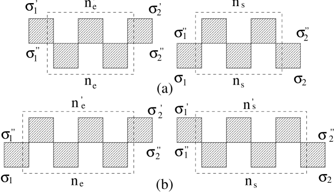
FIG. 2.: The superblock ${\cal T}_{M}$ is cut in a system ${\cal S}$ and environment ${\cal E}$ block for M=5 odd (a), M=6 even (b).

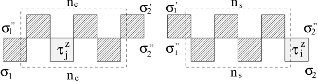
FIG. 3.: In the case $j=i$ or $i+1$, ${\cal T}_{M}^{ij}(k=2)$ is cut in ${\cal S}_{e}^{i}$ and ${\cal E}_{e}^{j}(k)$ for $M=6$, $i=1$.

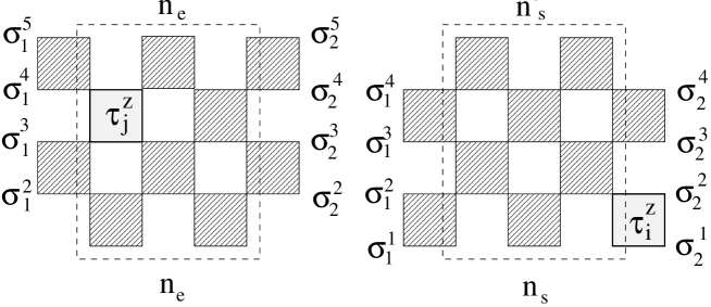
FIG. 4.: When $j.i+1$, additional internal $\sigma$ variables are needed in both ${\cal S}_{e}^{i}$ and ${\cal E}_{e}^{j}(k)$. Here, $i=1$, $j=3$ or $4$, $k=2$ and $M=6$.

FIG. 5.: Exact $G_{ii}(\tau)$ versus transfer matrix result with $m=100$ states. The thick solid line always represents the result extrapolated from the two finite $\epsilon$ values. In (a), $\epsilon=0.2$(dot-dashed), $0.1$(dotted) and in (b)-(d) $\epsilon=0.025$(dashed), $0.05$(thin solid).

FIG. 6.: XY model, $S^{z}_{ii}(\omega)$ using MaxEnt for the analytical continuation. The dotted line is the exact solution. The thin solid thin lines are obtained from the exact $G^{z}_{ii}(\tau)$.

FIG. 7.: XY model, $S^{x}_{ii}(\omega)$ from MaxEnt. In the transfer matrix DMRG calculations, $m=160$ states were kept and $\epsilon=0.025$. Inset: SK is gotten from the symmetric kernel and D1 includes $\frac{d}{d\tau}G(\tau)$.

FIG. 8.: Isotropic Heisenberg Model. MaxEnt from numerical data with $m=80$ and $\epsilon=0.025$.

FIG. 9.: Anisotropic model, $\Delta=2,4$. MaxEnt from numerical data with $m=100$ and $\epsilon=0.05$.

- [1] M. Takigawa, N. Motoyama ,H. Eisaki and S. Uchida Phys. Rev. Lett. 24 4612 (1996).
- [2] T. Imai etal., Phys. Rev. Lett. 81 220 (1998).
- [3] J. Jaklǐc and P. Prelovšek Phys. Rev. B 49, 5065 (1994).
- [4] V. S. Viswanath and G. Müller, Recursion method-Application to Many-Body Dynamics, Lecture Notes in Physics, Vol. 23 (Springer-Verlag, New York, 1994).
- [5] F. Naef and X. Zotos, J. Phys. C 10 L183-L190 (1998).
- [6] M. Böhm and H. Leschke Physica A 199 116 (1993).
- [7] K. Fabricius and B. McCoy, Phys. Rev. B 57, 8340 (1998).
- [8] O. A. Starykh, A. W. Sandvik and R. P. R. Singh, Phys. Rev. B 55, 14953 (1997).
- [9] R. J. Bursill, T. Xiang, G. A. Gehring, J. Phys. C 8, L583 (1996).
- [10] X. Wang and T. Xiang, Phys. Rev. B 56, 56 (1997).
- [11] N. Shibata, J. Phys. Soc. Jpn, 66, 2221 (1997).
- [12] K. Maisinger and U. Schollöck, Phys. Rev. Lett. 81, 445 (1998).
- [13] N. Shibata, B. Ammon, M. Troyer, M. Sigrist, K. and Ueda J. Phys. Soc. Jpn 67, 1086 (1998).
- [14] D. Coombes, T. Xiang, G. A. Gehring, J. Phys. C, to appear (1998); T. Xiang Phys. Rev. B to appear (1998).
- [15] S. Eggert and S. Rommer, Phys. Rev. Lett. 81, 1690 (1998).
- [16] K. Maisinger, U. Schollwöck, S. Brehmer, H. J. Mikeska and S. Yamamoto, Phys. Rev. B 58, R5908 (1998).
- [17] S. Yamamoto, T. Fukui, K. Maisinger, U. Schollwöck, J. Phys. C, (1998), to appear
- [18] X. Wang and T. Xiang, Thermodynamics of Hubbard chains, unpublished
- [19] A. Klümper, R. Raupach and F. Schönfeld, cond-mat/9809224
- [20] A similar extension has been reported in T. Mutou, N. Shibata and K. Ueda, Phys. Rev. Lett. 81, 4939 (1998).
- [21] M. Karbach et al., Phys. Rev. B 55, 12510 (1997).
- [22] A. H. Bougourzi, M. Karbach and G. Müller, Phys. Rev. B 57, 11429 (1998).
- [23] H.F. Trotter, Proc. Am. Math. Soc. 10, 545 (1959); M. Suzuki, Prog. Theor. Phys. 56, 1454 (1976).
- [24] H. Betsuyaku, Prog. Theor. Phys. 73 320 (1985).
- [25] S. R. White, Phys. Rev. Lett. 69, 2863(1992); R. Noack and S. R. White, The Density Matrix renormalization group in Lecture Note in Physics, Springer Velerg, eds. I. Peschel, X. Wang and K. Hallberg, (1998).
- [26] E.T. Jaynes, in Papers on Probability, Statistics and Statistical Physics, ed., R.D. Rosenkrantz, Reidel, Dordrecht, (1983).
- [27] S.F. Gull, in Maximum Entropy and Bayesian Methods, ed. J. Skilling, Kluwer Academic Publishers, Dordrecht, 53, 1989; J. Skilling,in Maximum Entropy and Bayesian Methods, ed. P.F. Fougère, Kluwer Academic Publishers, Dordrecht, 341, 1990.
- [28] G.L. Bretthorst, Bayesian Spectrum Analysis and Parameter Estimation, Springer Press, Berlin, Heidelberg, (1988) (can be downloaded from bayes.wustl.edu).
- [29] W. von der Linden, Appl. Phys. A 60, 155-165 (1995).
- [30] M. Jarrell, J.E. Gubernatis, Phys. Rep. 269, 133 (1996)
- [31] E. Lieb, T. Schulz and D. Mattis, Ann. Phys. 16, 407 (1961); B. M. McCoy, E. Barouch and D. B. Abraham, Phys. Rev. A 4, 2331 (1971).
- [32] T. Niemeijer, Physica 36, 377 (1967); S. Katsura, T. Horigushi and M.Suzuki, Physica 46, 67 (1970).
- [33] G. Müller and R. Shrock, Phys. Rev. B 29, 288 (1994).
- [34] A. R. Its, A. G. Izergin, V.E. Korepin and N.A. Slavnov, Phys. Rev. Lett. 70, 1704 (1993).
- [35] R. J. Baxter, J. Stat. Phys. 9, 145 (1973).
- [36] J. des Cloizeaux and M. Gaudin, J. Math. Phys. 7,1384 (1966).