Optimisation of on–line principal component analysis

Abstract

Various techniques, used to optimise on-line principal component analysis, are investigated by methods of statistical mechanics. These include local and global optimisation of node-dependent learning-rates which are shown to be very efficient in speeding up the learning process. They are investigated further for gaining insight into the learning rates’ time-dependence, which is then employed for devising simple practical methods to improve training performance. Simulations demonstrate the benefit gained from using the new methods.

1.Introduction

The investigation of unsupervised on-line learning algorithms [1, 2] by means of statistical mechanics has been shown to be a useful tool for gaining insight on the training dynamics [3]. In contrast to batch algorithms whereby all available examples are considered simultaneously for calculating a single student parameters update, on-line updates are carried out after the presentation of each single data point (for an overview on current on-line methods in neural networks see [4]). This update is proportional to a learning rate $\eta$ that has to be smaller than a critical value to make learning possible [5]. Successful learning is only possible if the learning rate is relatively small which, at the same time, means that many update steps are needed. Therefore, a relatively large rate is needed at the beginning and a smaller one later on; perfect learning is only possible if $\eta\rightarrow 0$ at late stages of the learning process. For practical problems there is only empirical knowledge of how the learning rate has to evolve [2]. The use of variational techniques [8, 9] enables one to calculate the optimal learning rate evolution $\eta$ theoretically; however, these calculations require information about the task and the input distribution which is usually unavailable. Nevertheless, insight gained from the analysis about the optimal learning rate time-dependence may be used to improve training in practical scenarios.

There are mainly two learning rate optimisation paradigms which we will discuss here: Local optimisation maximises the cost function loss at every time step while global optimisation seeks the maximisation of the cost function loss within a predetermined time window. Note that towards the end of the time window the two methods coincide and that a sufficiently long time window should be considered for the system to converge.

2. General Framework

The algorithm examined here is an on-line-algorithm for principle component analysis based on Sanger’s rule [6]. It was already discussed in detail for constant learning rates $\eta_{i}$ [7]. We consider here $N$-dimensional data vectors $\underline{\xi}$ taken independently from a Gaussian data-distribution with M relevant orthonormal directions $\{\underline{B_{i}}\}_{i=1,...,M}$ ($M\ll N$, $\underline{B}_{i}^{\top}\underline{B}_{j}\,=\delta_{ij}$). The correlation matrix $\underline{\underline{C}}=\left\langle\underline{\xi}\underline{\xi}^{\top}\right\rangle$ of this distribution has the form

$$\underline{\underline{C}}\,=\,\underline{\underline{I}}+\sum_{i=1}^{M}(b_{i}^{2}+2b_{i})\underline{B}_{i}\underline{B}_{i}^{\top}\ ,$$ (1)

were $\{b_{i}\}_{i=1}^{M}$ are some positive parameters representing the specific task and $\underline{\underline{I}}$ is the identity matrix.

In the on-line-scenario a single vector $\underline{\xi}^{\mu}$ is presented every time step and a set of student vectors $\underline{J}_{l}\in I\!\!R^{N}\quad(l=1,2,\ldots,M)$ is updated according to

$$\underline{J}_{l}(\mu)=\underline{J}_{l}(\mu-1)+\frac{\eta_{l}}{N}\,x_{l}^{\mu}\left(\underline{\xi}^{\mu}-\sum_{k=1}^{l}x_{k}^{\mu}\underline{J}_{k}(\mu-1)\right)\ ,$$ (2)

with the student projections $x_{l}^{\mu}=\underline{J}_{l}^{\top}\underline{\xi}^{\mu}$. The student vectors are normalized explicitly after each time step.

In the limit $N\rightarrow\infty$ the evolution of the system can be described by a set of coupled differential equations in ‘time’ $\alpha=\mu/N$ for the quantities $R_{kl}(\mu)=\underline{J}_{k}^{\top}(\mu)\underline{B}_{l}$ and $Q_{kl}(\mu)=\underline{J}_{k}^{\top}(\mu)\underline{J}_{l}(\mu)$ which describe the overlaps of the student vectors with the unknown principal components and the mutual overlap:

$$\frac{dR_{lj}}{d\alpha} = \eta_{l}\,\left\langle\,x_{l}y_{j}\,\right\rangle-(\eta_{l}+\eta_{l}^{2}/2)\,\left\langle\,x_{l}^{2}\,\right\rangle R_{lj}$$

$$-\eta_{l}\sum_{k=1}^{l-1}\,\left\langle\,x_{l}x_{k}\,\right\rangle(R_{kj}-Q_{lk}R_{lj})\ \ (k,l=1,2,\ldots,M)$$

$$\frac{dQ_{lm}}{d\alpha} = (\eta_{l}+\eta_{m})\,\left\langle\,x_{l}x_{m}\,\right\rangle-((\eta_{l}+\eta_{l}^{2}/2)\,\left\langle\,x_{l}^{2}\,\right\rangle+(\eta_{m}+\eta_{m}^{2}/2)\,\left\langle\,x_{m}^{2}\,\right\rangle)Q_{lm}$$

$$-\eta_{l}\sum_{k=1}^{l-1}\,\left\langle\,x_{l}x_{k}\,\right\rangle(Q_{km}-Q_{kl}Q_{lm})-\eta_{m}\sum_{k=1}^{m-1}\,\left\langle\,x_{m}x_{k}\,\right\rangle(Q_{lk}-Q_{km}Q_{lm})\ (l\neq m)\ .$$

The averages over the quantities $x_{k}=\underline{J}_{k}^{\top}\underline{\xi}$ and $y_{j}=\underline{B}_{j}^{\top}\underline{\xi}$ can be performed analytically yielding

$$\,\left\langle\,x_{k}y_{j}\,\right\rangle=(1+b_{j})^{2}R_{kj},\quad\,\left\langle\,y_{i}y_{j}\,\right\rangle=(1+b_{j})^{2}\delta_{ij},\mbox{~{}~{}and~{}~{}}$$ (4)

$$\,\left\langle\,x_{k}x_{l}\,\right\rangle=Q_{kl}+\sum_{i}^{M}(b_{i}^{2}+2b_{i})R_{ki}R_{li}\ .$$

An investigation of this learning scenario with constant learning rates showed that the entire process depends crucially on the learning rate. Learning rates have to be slightly different for each student vector to break symmetries which emerge between them during training and to avoid time-consuming plateaus [7]. The values have to be chosen between large learning rates which are suboptimal asymptotically and small learning rates that result in prohibitively slow learning at the transient.

To improve learning performance and speed it is necessary to choose time-dependent learning rates. As it was already shown that different learning rates for different nodes are important [7] we focussed on finding appropriate solutions for a node-dependent learning rates $\eta_{l}(\alpha)$.

3. Locally Optimised Learning Rate

One way to calculate an optimised learning rate is to maximise the cost function loss in every time-step (local optimisation), i.e., obtaining $\eta_{i}(\alpha)$ from a minimisation of $d\epsilon/d\alpha$ [8]:

$$\frac{\partial}{\partial\eta_{l}}\frac{d\epsilon}{d\alpha}=0\ ,$$ (5)

Choosing the cost function

$$\epsilon=1-\frac{1}{M}\sum^{M}_{l=1}R_{ll}^{2}\ .$$ (6)

This function is a measure of the learning success on a scale between 1 and 0, representing poor and optimal performance respectively, and may be used to derive the locally optimal learning rate of the form

$$\eta_{l}(\alpha)=-1+\frac{(1+b_{l})^{2}}{(1+A_{ll})}-\frac{\sum_{k=1}^{l-1}(Q_{lk}+A_{lk})(R_{kl}-Q_{kl}R_{ll})}{(1+A_{ll})R_{ll}}\ ,$$ (7)

with

$$A_{kl}=\sum_{i=1}^{M}(b_{i}^{2}+2b_{i})R_{ik}R_{il}\ .$$

Figure 1: Time-dependence of the learning rates of the first three students calculated with local optimisation.

Figure 2: Overlap of the first three students with their principal components and their mutual overlap, learning with the the locally optimised learning rates shown above.

Figure 3: Cost functions for the detection of the first three components in on-line PCA: the graph shows the learning process with constant learning rates (a), with locally optimised (b) and with globally optimised (c) learning rates.

This learning rate depends on the data structure and the order parameters of the problem. By choosing these optimal learning rates, the principal components are learnt very fast and high performance can be achieved. In the following we choose a data distrbution (1) with $b_{1}=0.6$, $b_{2}=0.4$ and $b_{3}=0.3$. Figure 1 shows the evolution of the learning rates for the first three student vectors. They all begin with a constant value which depends on the data structure and have a decaying phase later on where the learning rate decays roughly as $1/\alpha$. In addition, the learning rates show a ‘dip’ at the point where another student vector learns the current, most-dominant, principal component direction. This behaviour is explained by Figure 2, showing the overlaps $R$ of the students with the principal components (upper curves) and their mutual overlap $Q$ (lower curves): The principal components are learned one after another; all students try to learn the largest p.c. first, which results in a significant overlap $Q$ with the first student. The orthogonalisation realised by the algorithm pushes the other students away from that direction to specialise on other directions related to the less dominant p.c. Once the direction of the p.c. has been identified, the related learning rate, of the specialised student vector, starts decaying. At the same time there is a significant overlap with the other student vectors that started learning the same direction; consequently, their learning rates are suppressed so as to prevent them from specialising on this p.c. any further and to facilitate the change in direction.

Figure 3 shows the evolution of the cost function(6). Curve (a) represents a learning scenario with reasonably chosen constant learning rates ($\eta_{1}=0.1$, $\eta_{2}=0.108$ and $\eta_{3}=0.09$) balancing between training speed and asymptotic performance. The hierarchical structure of the learning process can be noticed here as the three students learn the different principal components one after the other. The same learning process but with locally optimised learning rates is shown in curve (b). The principal components are learned very fast, resulting in very good asymptotic performance. The locally optimised learning rate clearly provides improved performance with respect to every constant rate. However, it depends on knowledge that is not available in practical situations and can therefore only provide insight into the optimal evolution of $\eta_{l}$.

4. Globally Optimised Learning Rate

As the learning process may comprise different phases, for which local optimisation may result in sub-optimal global performance, we will also consider here a different approach based on global optimisation [9] of the learning rate. This has been shown to outperform local optimisation over a predetermined time window. This method maximises the cost function loss over a fixed time window:

$$\Delta\epsilon=\int^{\alpha_{1}}_{\alpha_{0}}d\alpha\ \left(\frac{d\epsilon}{d\alpha}-\sum_{i}\lambda_{i}\ (\mbox{constraints})\right)$$ (8)

where the constraints are the equations of motion (Optimisation of on–line principal component analysis ) which have to be satisfied at every point in time and $\lambda_{i}$ are the related Lagrange multipliers. The time-window $\alpha_{1}\!-\!\alpha_{0}$ has to be chosen beforehand. Applying a variational approach with respect to the order parameters and their time derivatives leads to a set of differential equations for the Lagrange multipliers, from which the globally optimised learning rates $\eta_{i}$ can be derived. Clearly, like in any other method, a minimal time-window is required for the learning to converge.

Globally optimal parametrisation was shown to be much more efficient in the case of plateaus in the learning process where local optimisation leads to indefinite trapping [9]. However, one has to keep in mind that global optimisation only looks at the total loss $\Delta\epsilon$, so that intermediate values of $\epsilon$ can be much worse than those obtained via local optimisation. In the case of on-line-PCA it turns out that that after the minimal time needed for the algorithm to converge, the learning performance of locally and globally optimised learning are similar. Figure 3 shows the evolution of the learning process in both cases.

One can notice that the principal components are found later than with local optimisation. This can be explained in the following way: If one component is found more accurately, the orthogonalisation process can push the other students much more efficiently out of that direction, so that learning the next p.c. becomes easier. Local optimisation does not rely on future gains and therefore chooses to carry on with the specialisation of student vectors, providing better intermediate performance. The features of the globally optimised learning rates are similar to those obtained via local optimisation.

Global optimisation would have been useful in the case of plateaus; these emerge in the case of on-line-PCA only for a single learning rate $\eta_{i}(\alpha)=\eta(\alpha)$ [7]. Therefore, in most cases, global optimisation will not have any advantage over local optimisation.

Note that instead of calculating a globally optimised learning rate that leaves the learning rule itself unchanged, one can also calculate a globally optimised learning rule [10]. In our case this can only be calculated numerically and does not provide additional information.

5. Discussion

The use of locally optimised learning rates shows a significant improvement in the learning performance over fixed learning rates, but it depends on quantities that are not available in practical applications of on-line-PCA. Nevertheless, insight gained from the theoretical study may be useful for improving performance in practical cases. From the analysis it is clear that the learning rates have to be constant first and should decay like $1/\alpha$ at later times, after specialisation took place. This point, where the learning rate schedule should be changed has to be set through observables accessible in practical scenarios; typically, one could use constant learning rates until the asymptotic regime is reached, identified through students stationarity. Our analysis provides a refined criterion which leads to much faster learning: In figure 1 and 2 on notices that the decaying phase for a certain student starts where the overlap to other students (usually to one in particular) starts growing significantly. At this point the first student has already learned the current most-dominant p.c. and becomes almost stationary while other students (one in particular), which show significant correlation with the first student, should start moving to other directions, being pushed away by the orthogonalisation process. The first student has learned enough to stabilise and to begin its ‘fine tuning’ which corresponds to the stage of a decaying learning rate. The mutual overlaps are the only order parameters accessible in real applications; here they provide a practical criterion for the starting point of the learning rate decay phase, a criterion which was obtained directly from the analysis.

6. Simulation

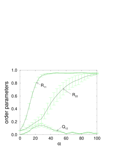
Figure 4: Simulation of on-line-PCA with constant learning rates: Overlaps of the first two students with their PC’s $R_{ll}$ and their mutual overlap $Q$.

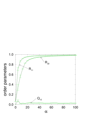
Figure 5: Simulation of on-line PCA like in figure 4. The learning rates are now chosen as time-dependent according to the suggested rule. A comparison with figure 4 demonstrates clearly the efficiency of this method.

Simulations of an on-line principle component analysis were made to test the usefulness of the criterion explained above. Fig 4 displays a scenario with constant learning rates ($\eta_{1}=0.1$ and $\eta_{2}=0.09$), learning the same data distribution as before. The graph shows the overlaps of the first two students with the corresponding principal components $R_{ll}$ and their mutual overlap $Q$ as means and variances of ten runs. The asymptotic regime is reached at the end of the time scale; at this point one would normally commence the decay of the learning rates. In comparison, we applied the rule suggested above, based on monitoring the overlaps between student vectors, to the same task as shown in figure 5. As soon as the overlap between two students starts growing significantly the decay of the first student commences; the decay for the next student commences according to similar criteria. This corresponds directly to the observations of the optimised learning process. We should point out that the starting value of the learning rates can be chosen higher than those in the constant case since the decay starts very early. This demonstrates the efficiency of the rule developed here which is applicable to practical scenarios.

7. Conclusion

A statistical mechanics approach to optimising on-line principal component analysis provides insight to the learning process. The theoretically obtained time-dependent optimal learning rates depend on quantities which are not accessible in practical applications; however, examining the optimal learning scenarios led to the development of a practical technique for speeding up the training process on the basis of observables that can be easily monitored in practical scenarios. The new method has been demonstrated on a simple problem and was shown to improve the training performance considerably.

Acknowledgments  This work has been partially support by the EU grant CHRX-CT92-0063 and the British Council grant: British-German Academic Research Collaboration Programme project 1037. DS also acknowledges support from the Leverhulme Trust (F/250/K). ES and DS would like to thank Magnus Rattray for usefull discussions and suggestions.

References

- [1] J Hertz, A Krogh and R Palmer Introduction to the Theory of Neural Computation , Addison–Wesley, Redwood City, CA (1991)
- [2] C Bishop Neural Networks for Pattern Recognition, Clarendon Press, Oxford (1995)
- [3] M Biehl, Europhys. Lett. 25 (1994) 391 Neurocomp. 5 (1993) 185
- [4] D Saad (ed) On-line Learning in Neural Networks, Cambridge University Press, Cambridge UK (1998)
- [5] T Watkin, A Rau, and M Biehl, Rev.Mod.Phys. 65 (1993) 499
- [6] T Sanger, Neural Networks 2 (1989) 549
- [7] M Biehl and E Schlösser, J. Phys. A 31 (1998) 79
- [8] O Kinouchi and N Caticha, J. Phys. A 25 (1992) 6243
- [9] D Saad and M Rattray, Phys. Rev. Lett. 79 (1997) 2578 ; M Rattray and D Saad, Phys. Rev. E 58 (1998) 6379
- [10] M Rattray and D Saad, J. Phys. A 30 (1997) 771