Critical properties and phase diagram
of the quantum anisotropic $XY$ spin chain in a random magnetic field:
A density-matrix renormalization-group analysis

Abstract

The spin-1/2 quantum anisotropic $XY$ spin chain in a transverse random magnetic field parallel to the $z$ axis is numerically studied by means of the density-matrix renormalization group. The dependence of the spontaneous magnetization and the energy gap on both the strength of the random magnetic field and the factor of anisotropy is determined. The critical line for the order-disorder phase transition is obtained and the resulting phase diagram is drawn. Our results are compatible with the fact that models with different factors of anisotropy fall within the same universality class as the quantum Ising model in a transverse random field. PACS numbers: 75.10.Jm, 75.40.Mg, 05.50.+q

]

I Introduction

The effect of disorder on quantum systems is more intriguing than its classical counterpart, especially when the random noise does not directly affect the interactions in the original system, but is coupled to other degrees of freedom, which have nontrivial commutation relations with the degrees of freedom appearing in the original Hamiltonian. A simple example within this class of systems is provided by the transverse randomness in an easy-axis or easy-plane quantum spin chain. Indeed, when the exchange interactions involve the $x$ and $y$ spin components, a random magnetic field coupled to the $z$ spin component produces dramatic effects due to the nontriviality of the angular-momentum algebra.

In this paper we analyze the one-dimensional spin-1/2 quantum anisotropic $XY$ model in a transverse random magnetic field, which is defined by the Hamiltonian

$${\cal H}= - J\sum_{\ell=1}^{N-1}S_{\ell}^{x}S_{\ell+1}^{x}-\gamma J\sum_{\ell=1}^{N-1}S_{\ell}^{y}S_{\ell+1}^{y}$$ (1)

$$- \sum_{\ell=1}^{N}h_{\ell}S_{\ell}^{z}-h_{x}\sum_{\ell=1}^{N}({\rm sgn}J)^{\ell}S_{\ell}^{x},$$ (2)

where $N$ is the number of sites in the chain,

$$\matrix{S_{\ell}^{\alpha}=&\sigma^{0}&\otimes&\ldots&\otimes&\sigma^{\alpha}/2&\otimes&\ldots&\otimes&\sigma^{0}\cr~{}&1&~{}&\ldots&~{}&\ell&~{}&\ldots&~{}&N}$$

are the spin-1/2 operators acting on the Hilbert space spanned by the vectors $|\psi_{1},\ldots,\psi_{\ell},\ldots,\psi_{N}\rangle$, $\{\psi_{\ell}\}$ are two-component spinors, $\sigma^{0}$ is the $2\times 2$ identity matrix, $\{\sigma^{\alpha}\}$ are the $2\times 2$ Pauli matrices, $\otimes$ is the symbol for tensor product, $J$ is the coupling constant for the $x$ spin components, $\gamma$ is the factor of anisotropy, $\gamma J$ is the coupling constant for the $y$ spin components, and $\{h_{\ell}\}$ are the on-site values of a random magnetic field directed along the $z$ axis, which are uniformly distributed in the interval $-h_{0}\leq h_{\ell}\leq h_{0}$. In the following we call $h_{0}$ the strength of the random magnetic field.

Due to the conventions adopted in Eq. (2) a positive (negative) coupling constant stands for a ferromagnetic (antiferromagnetic) coupling. Correspondingly the external field $h_{x}$ directed along the $x$ axis, which we include in our model to force spontaneous symmetry breaking along the easy axis of magnetization, is uniform (staggered) when $J$ is ferromagnetic (antiferromagnetic).

In principle the coupling constant $J$ and the factor of anisotropy $\gamma$ have arbitrary signs, and the only implicit limitation in Eq. (2) is $-1\leq\gamma\leq 1$, which amounts to defining the $x$ and $y$ axes according to the relative strength of the exchange interaction. However the local gauge transformations $S_{\ell}^{x}\to({\rm sgn}J)^{\ell}S_{\ell}^{x}$, $S_{\ell}^{y}\to({\rm sgn}J{\rm sgn}\gamma)^{\ell}S_{\ell}^{y}$, and $S_{\ell}^{z}\to({\rm sgn}\gamma)^{\ell}S_{\ell}^{z}$ make all the coupling constants ferromagnetic and the external field $h_{x}$ uniform, while preserving the commutation relations among the spin operators, i.e. the orientation of the local reference frames is preserved by the transformations. We take then the units of energy such that $J=1$, and only consider the case $0\leq\gamma\leq 1$. We also assume that $h_{x}\geq 0$. It is important to observe that the gauge transformations change the random field as $h_{\ell}\to({\rm sgn}\gamma)^{\ell}h_{\ell}$, which is again uniformly distributed in the interval $[-h_{0},h_{0}]$. However, unlike the Ising limit ($\gamma=0$), at finite $\gamma$ there is no freedom left to make all the $\{h_{\ell}\}$ positive (cf. Ref. [1]), because any further local gauge transformation will not keep fixed both the sign of the coupling constants and the orientation of the local reference frames.

The outline of the paper is the following. In Sec. II we briefly recapitulate some previously established results in the two limiting cases: the $XY$ model in the absence of randomness and the quantum Ising model in a transverse random field. The main scope of Sec. II is to provide a framework to which to refer in the discussion and the interpretation of the results obtained in this paper. In Sec. III we discuss some technical aspects which are fundamental to obtain well-defined numerical results, and their relation to the physical properties of the model. This discussion is essential to allow for the reproducibility of our results, and to shed light on the physics underlying the DMRG algorithm. In Sec. IV we determine the critical properties and the phase diagram of the model (2) in the $h_{0}$ vs $\gamma$ plane. A summary of the principal results and some concluding remarks are found in Sec. V.

II Some limiting cases

The model (2) with a generic $\gamma$ is integrable in the absence of randomness and external magnetic field ($h_{0}=0$, $h_{x}=0$)[2] by fermionization of the spin operators.[3] The particle-hole excitation spectrum of the corresponding fermionic system shows, in particular, that the ground state is separated from the first excited state by an energy gap[4]

$$G_{0}=1-\gamma$$ (3)

(in units of $J$). In the thermodynamic limit the spectrum above the gap is continuous and the ground-state energy per site is

$${\cal E}_{0}^{{\rm theo}}=-(1+\gamma)\int_{-\pi}^{\pi}{dk\over 8\pi}\left[1-\frac{4\gamma\sin^{2}k}{(1+\gamma)^{2}}\right]^{1/2}.$$ (4)

A pictorial representation of the physics of the $XY$ model is provided by the spin wave (SW) theory, which is qualitatively correct (in a sense that will be clearer in the following), except for $\gamma$ very close to 1. Expressing the spin operators in terms of auxiliary boson operators $a_{\ell},a_{\ell}^{+}$ according to $S_{\ell}^{x}={1\over 2}-a_{\ell}^{+}a_{\ell}$, $S_{\ell}^{y}={1\over 2}(a_{\ell}^{+}+a_{\ell})$, and retaining only bilinear terms, the Hamiltonian (2) is cast in a diagonal form by a Fourier transform from real-space to $k$-space representation, and by a subsequent canonical Bogoliubov transformation. The resulting SW excitation spectrum is $\varepsilon_{k}=\sqrt{1-\gamma\cos k}$, and the ground-state energy per site in the thermodynamic limit is

$${\cal E}_{0}^{\rm SW}=-{3\over 4}+\int_{-\pi}^{\pi}{dk\over 4\pi}\sqrt{1-\gamma\cos k}.$$

I.e., the gap in the excitation spectrum is $G_{\rm SW}=\sqrt{1-\gamma}$, which coincides with (3) only in the Ising limit $\gamma=0$ and in the isotropic limit $\gamma=1$, and is not even perturbatively correct at small $\gamma$. Nonetheless the discrepancies are mostly quantitative and the SW theory may be adopted as a reference theory to discuss the physics of the $XY$ model. In particular, at $\gamma>0$, the SW Hamiltonian includes a contribution from the zero-point motion of elementary excitations. The reduction of the spontaneous magnetization with respect to the saturation value $M_{0,max}={1\over 2}$ in the Ising limit ($\gamma=0$) is understood within SW theory as the effect of such quantum fluctuations for $\gamma>0$. Indeed the SW result for the spontaneous magnetization is

$$M_{0}={1\over 2}-\int_{-\pi}^{\pi}{dk\over 8\pi}\displaystyle{2-\gamma\cos k-2\sqrt{1-\gamma\cos k}\over\sqrt{1-\gamma\cos k}}.$$ (5)

This result is meaningless at $\gamma=1$ due to the divergence of the integral in the r.h.s., a fact which is used as an evidence against the existence of a spontaneous magnetization in the isotropic $XY$ model. However, due to the logarithmic nature of the divergence, it turns out that the reduction of the magnetization associated with SW zero-point motion is an underestimate of the reduction in the exact ground state (see Eq. (10) and text below it), except for $\gamma$ very close to 1. Thus in the following, for the sake of definiteness, we adopt the SW language and we conventionally refer to the effects of the anisotropy as resulting from quantum fluctuations with respect to an Ising-like ground state, as it would be in a more refined (i.e. beyond SW) field theoretical approach to the $XY$ model.

As a consequence of the gap in the excitation spectrum the quantum fluctuations are massive. The spins are ordered and the system is ferromagnetic (FM) for $\gamma<1$. In the isotropic limit $\gamma=1$ (the so-called $XX$ model), the gap closes and the spontaneous magnetization is driven to zero, by massless phase fluctuations. The system is thus paramagnetic (PM). It is worth mentioning that in the isotropic limit the model is equivalent to a model of hard-core bosons, and the absence of spontaneous magnetization in the magnetic system is related to the absence of Bose-Einstein condensation in the corresponding one-dimensional interacting boson system.

The issue addressed in this paper is the evolution of the magnetic ground state for $\gamma<1$ in the presence of the transverse randomness introduced by a random magnetic field along the $z$ axis. In particular we want to study the interference between the critical behavior driven by $\gamma\to 1$ and the critical behavior controlled by the random field $h_{0}$. Indeed, in the extreme anisotropic case $\gamma=0$[5, 6] the system undergoes a FM-PM quantum phase transition.[7] The magnetization at the critical point $h_{0}=h_{c}\equiv{\rm e}/2=1.3529\ldots$ is a nonanalytical function of the external field $h_{x}$,[8] $M\left(h_{0}=h_{c},h_{x}\right)\sim\left[\ln\left(D_{h}/h_{x}\right)\right]^{\phi-2}$, where $\phi=(1+\sqrt{5})/2=1.618\ldots$  is the golden mean and $D_{h}$ is a scale factor. The spontaneous magnetization $M_{0}\equiv M(h_{x}\to 0)$ in the ordered phase decreases with increasing $h_{0}$, and

$$M_{0}\sim(h_{c}-h_{0})^{2-\phi}$$ (6)

for $h_{0}\to h_{c}^{-}$. Contrary to ordinary continuous phase transitions, where the nonanalyticity is limited to the critical point, a Griffiths’ region[9] exists around the critical point, where $M(h_{x})$ is not analytical. In the weakly ordered Griffiths’ region ($h_{0}<h_{c}$), for small $h_{x}$,

$$M(h_{x})-M_{0}\sim h_{x}^{\alpha}\left[\ln\left(D_{h}^{\prime}/h_{x}\right)\right]^{\kappa},$$ (7)

where $M_{0}$ is the spontaneous magnetization, the exponent $\kappa$ cannot be determined within renormalization group, $D_{h}^{\prime}$ is a nonuniversal scale factor, and the exponent $\alpha$ depends continuously on the distance from criticality $\delta\sim h_{c}-h_{0}$. [7] As far as $\alpha\leq 1$, the spin susceptibility diverges as $h_{x}\to 0$, i.e. the magnetization curves intercept the axis $h_{x}=0$ with an infinite slope, even when $M_{0}$ is finite.

Previous results of density-matrix renormalization-group (DMRG) calculations at $\gamma=0$[1] were in good agreement both with the theory[5, 6, 7] and other numerical calculations.[10] Below we extend these results to the entire region $h_{0}>0$, and $0\leq\gamma\leq 1$, and determine the full phase diagram and the critical properties of the model (2). We are interested in understanding the role of quantum fluctuations (in the sense clarified above) in the Griffiths’ region. The issue is particularly intriguing for $\gamma\to 1$, when the critical behavior of the nonrandom system interferes with the critical behavior controlled by the random field. This interference is directly evident in those quantities which vanish at criticality, such as the spontaneous magnetization and the gap in the excitation spectrum.

We point out that, due to the iterative nature of the infinite-size DMRG algorithm, the system size is increased while the irrelevant states are progressively truncated away. The discrepancy between the infinite-size limit of the algorithm and the thermodynamic limit of the physical system depends on the size of the error introduced by the truncation.[11] Thus the technical aspects related to the definition of a proper numerical procedure are deeply entangled with the physical properties of the system. In particular it will be clear that, in order to drive the system towards the phase transition, it is not only necessary to reach the infinite-size limit, in the presence of an infinitesimal external field, but it is also important to control and determine the effect of the truncation of the Hilbert space. The full procedure explained below is essential to reproduce our results and obtain the correct limiting behaviors.

III Algorithm and technicalities

We perform our calculations using the infinite-size DMRG algorithm introduced by White[11] with some minor modifications described in Ref. [1]. Accordingly, we adopted open boundary conditions, which produce more accurate results within DMRG.[11]

At a fixed number $s$ of states kept in the truncation of the density matrix and after a (sufficiently large) fixed number $N_{\rm RG}$ of DMRG steps, when the chain consists of $N=2N_{\rm RG}+2$ sites, the magnetization at a given (small) uniform magnetic field $h_{x}$ decreases both with the strength of the random field $h_{0}$ and the factor of anisotropy $\gamma$, except for a region close to $\gamma=1$ where the magnetization appears to be a nonmonotonic function of $h_{0}$ (see Fig. 1). The strong dependence of the magnetization on the external field around the critical point is essentially the result of a divergent susceptibility in the Griffiths’ region. Even for a field as small as $h_{x}=10^{-5}$, the transition point is masked by the strongly nonanalytical behavior, and is only hinted by the change in the curvature of the $M$ vs $h_{0}$ curves.

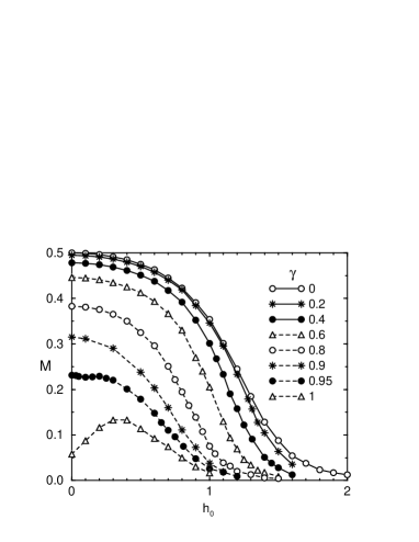
FIG. 1.: The dependence of the magnetization on the random magnetic field for different values of the factor of anisotropy $\gamma$. The system size is 302 sites, the uniform magnetic field $h_{x}=10^{-5}$, and eight states are kept at each DMRG step. The large value of the magnetization in the disordered region is essentially due to the anomalous response to the external field $h_{x}$ in the Griffiths’ region.

Moreover, it is evident that particular care has to be exercised close to the isotropic limit $\gamma=1$, to extract the correct behavior. Indeed, quantum fluctuations suppress the spontaneous magnetization at $\gamma=1$ even in the absence of randomness. Thus we expect $M_{0}$ to be zero for all values of $h_{0}$. This indicates that a proper procedure has to be defined, which is reliable and unique for all $\gamma$. We carefully address this issue and the results are given below.

To determine the spontaneous magnetization a (small) uniform magnetic field $h_{x}$ in the $x$ direction is applied to lift the degeneracy in the ground state, which is doubly degenerate at $h_{x}=0$ (this degeneracy occurs for large system sizes for $\gamma>0$ and for any size at $\gamma=0$). Usually, for small values of $\gamma$, any $h_{x}$ is enough to truncate the undesired degenerate state after the initial DMRG steps. However, the closer one gets to $\gamma=1$, the larger this uniform field should be, and more than 150 DMRG steps could be needed to isolate the state with broken symmetry. Further, increased accuracy of calculations (i.e. a larger number of states kept) is also needed close to $\gamma=1$. We have checked that the difference between the exact ground-state energy ${\cal E}_{0}^{{\rm theo}}$, given by Eq. (4), and the calculated one ${\cal E}_{0}^{{\rm DMRG}}$ for a fixed number of states kept in the truncation procedure, $s=8$, closely follows the truncation error[11] $1-P_{s}=1-\sum_{m=1}^{s}\varrho_{m}=\sum_{m>s}\varrho_{m}$, i.e. the sum of the eigenvalues of the density matrix which correspond to the truncated states. This error increases with increasing $\gamma$, from $10^{-13}$ at $\gamma=0$, to $10^{-4}$ at $\gamma=1$. This phenomenon is deeply related to the increasing complexity of the ground state, as the role of quantum fluctuations is emphasized. As a consequence, the spontaneous magnetization has a dependence on the parameters $s$ and $N_{\rm RG}$ which becomes more and more important as $\gamma\to 1$.

To deal with this dependence and obtain the correct spontaneous magnetization $M_{0}=M(h_{x}\to 0)$ for all $\gamma$, the following steps are needed: (i) We calculate the magnetization along the easy axis

$$M_{j}^{(s)}(N_{\rm RG},h_{x},h_{0})=(2N_{\rm RG}+2)^{-1}\times$$

$$\langle h_{x},h_{0};N_{\rm RG},s,j|{\tilde{S}}^{x}|h_{x},h_{0};N_{\rm RG},s,j\rangle,$$ (8)

where $\langle\,\cdot\,\rangle$ is the quantum expectation value in the ground state and ${\tilde{S}}^{x}$ is the properly truncated total $x$-spin operator, at each DMRG step $N_{\rm RG}$, for a given uniform magnetic field $h_{x}$ and a random magnetic field of strength $h_{0}$, while $s$ states are kept during the DMRG procedure. The index $j$ labels a particular realization of the random field. Then (ii) we average this value over $N_{c}$ realizations of the random field, $\overline{M}^{(s)}(N_{\rm RG},h_{x},h_{0})=N_{c}^{-1}\sum_{j=1}^{N_{c}}M_{j}^{(s)}(N_{\rm RG},h_{x},h_{0})$, where a suitable value for $N_{c}$ depends on both $\gamma$ and $h_{0}$. In most cases an average over $N_{c}=500$ configurations gives satisfactory results, though sometimes more than 2000 configurations are needed (for $\gamma\simeq 1$ and close to criticality).

Due to the effects of the edges of the chain, $\overline{M}$ always increases with increasing lattice size, but the increase is very slow above some typical chain size ($N_{\rm RG}=50$), and may be fitted as $\overline{M}^{(s)}(N_{\rm RG},h_{x},h_{0})=\overline{M}^{(s)}(\infty,h_{x},h_{0})-A/N_{\rm RG}$, where $A$ and $\overline{M}^{(s)}(\infty,h_{x},h_{0})$ are fitting parameters, and so (iii) we extrapolate $\overline{M}$ to the infinite-size limit $N_{\rm RG}\to\infty$ and obtain $\overline{M}^{(s)}(\infty,h_{x},h_{0})$.

The larger the number of states $s$ kept is, during renormalization, the better the accuracy obtained is, so the magnetization slightly decreases with $s$ (a qualitative argument is: the smaller the number of states kept is, the more influential the state with all spins up is, the larger $M$ is). Thus (iv) we make an extrapolation to $s=\infty$, [11] using the formula

$$\overline{M}^{(s)}(\infty,h_{x},h_{0})=\overline{M}^{(\infty)}(\infty,h_{x},h_{0})+B\times\left({1\over s}\right)^{k},$$ (9)

which fits the data quite well (except for small oscillations at larger $1/s$), and we obtain $\overline{M}^{(\infty)}(\infty,h_{x},h_{0})$, (see Fig. 2). A more accurate formula is slightly different. On physical grounds, indeed, one expects that the magnetization $M(1/s)\equiv\overline{M}^{(s)}(\infty,h_{x},h_{0})$ consists of two parts: $M(1/s)=M_{{\rm reg}}(1/s)+M_{{\rm noise}}$, where the regular part $M_{{\rm reg}}(1/s)$ has a Taylor expansion close to $1/s=0$ and the noise part $M_{\rm noise}$ is due to nonuniform changes in the ground-state properties and only exists at large $1/s$. As the field $h_{x}$ is increased, the dependence on $1/s$ becomes much weaker (in strong fields the ground state is fully magnetized and so $s=1$ gives the exact solution), which means that for large fields one expects $M(1/s)$ to be a noiseless horizontal line, which can be imagined as resulting from a successive vanishing of the terms in the Taylor expansion of $M_{\rm reg}(1/s)$. Indeed, a Taylor expansion up to fifth order shows that only the fourth order $1/s$ term has any influence for the $h_{x}=4\times 10^{-3}$ data (Fig. 2), though both the linear and square $1/s$ terms are present for $h_{x}=1\times 10^{-4}$. The fact that no more than two nonconstant terms are ever present in the Taylor expansion for any of the chosen $h_{x}$ allows us to introduce with sufficient accuracy the effective formula (9), which is desirable because of a smaller number of free parameters. The presence of two (nonconstant) terms in the Taylor expansion at small $1/s$ results in a noninteger exponent $k$ in Eq. (9), where only one power is considered. The exponent $k$ is intermediate between the two corresponding integer exponents appearing in the Taylor expansion.

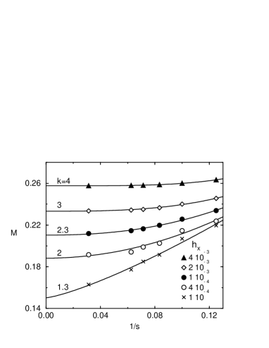
FIG. 2.: The dependence of the magnetization (extrapolated to $N_{\rm RG}\to\infty$) on the inverse number of states kept, $1/s$, at $\gamma=1$, in the absence of randomness, $h_{0}=0$. The solid lines are fits of the form $M=M(0)+B\times(1/s)^{k}$, the values of the exponent $k$ are shown.

Finally, (v) we extrapolate $\overline{M}^{(\infty)}(\infty,h_{x},h_{0})$ to zero external field $h_{x}$, using the expression $\overline{M}^{(\infty)}(\infty,h_{x},h_{0})=\overline{M}^{(\infty)}(\infty,0,h_{0})+Ch_{x}^{\alpha}$, where $C$ is a fitting parameter, $M_{0}(h_{0})\equiv\overline{M}^{(\infty)}(\infty,0,h_{0})$ is the spontaneous magnetization as a function of $h_{0}$ (at fixed $\gamma$) and the exponent $\alpha$ is determined by the fit to numerical data and is smaller than 1 in the Griffiths’ region, where the susceptibility diverges as $h_{x}\to 0$. The above formula is a slight modification of Eq. (7), based on the observation that the exponent $\kappa$ is negligible. The modified formula reproduces the behavior of numerical data for any value of the factor of anisotropy $\gamma$. As Fig. 3 shows, the magnetization is decreasing with increasing $h_{0}$, and we clearly see that $M_{0}$ goes to zero at $\gamma=1$ even though the uncertainty is rather large which is due to that we are exactly at criticality, e.g. $M_{0}(h_{0}=0)=-0.18\pm 0.18$, when properly extrapolated.

FIG. 3.: The dependence of the magnetization (extrapolated to $N_{\rm RG}\to\infty$, $s\to\infty$) on the uniform magnetic field $h_{x}$ at $\gamma=1$. The lines are fits of the form $M=M_{0}+Ch_{x}^{\alpha}$.

We point out that the above successive extrapolations are not needed in the Ising limit ($\gamma=0$) Ref. [1] and add but little accuracy for small $\gamma$. This is due to the fact that the truncation error decreases very rapidly as a function of the number $s$ of states kept when $\gamma$ is small. Thus, provided the system size is reasonably large and $s$ not too small, the only extrapolating procedure needed to get the correct behavior for the spontaneous magnetization, close to the Ising limit, is $h_{x}\to 0$.[1]

IV Results and discussion

As a starting test for the procedure discussed in Sec. III, we have calculated the spontaneous magnetization $M_{0}$ for many different values of $\gamma$ at zero random field. As we anticipated, quantum fluctuations tend to reduce the magnetization. We fitted our data as

$$M_{0}(h_{0}=0,\gamma)={1\over 2}(1-\gamma^{2})^{\vartheta},$$ (10)

with $\vartheta=0.255^{+0.010}_{-0.005}$, very close to $1/4$ (the circles in Fig. 4), which is to be compared to the SW result Eq. (5) (the dashed line in Fig. 4). In SW language, the factor $(1-\gamma^{2})^{\vartheta}$ represents the reduction of the magnetization, with respect to the saturation value $M_{0}(h_{0}=0,\gamma=0)=1/2$, due to quantum fluctuations. This factor is independent of the sign of $\gamma$, and drives the spontaneous magnetization to zero as $\gamma\to 1$. Thus, even in the absence of randomness, a critical behavior is induced by quantum fluctuations. This behavior interferes with the critical behavior controlled by the random field.

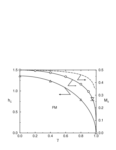
FIG. 4.: The triangles represent the critical points $h_{c}$ obtained by DMRG calculations for different values of the factor of anisotropy $\gamma$. The solid line is the best fit of the form $h_{c}=h(0)(1-\gamma^{2})^{\varrho}$ with $\varrho=0.52\pm 0.01$. The system is in a ferromagnetic state below this line. The circles represent the dependence of the spontaneous magnetization on $\gamma$ at $h_{0}=0$. Data are fitted by $M_{0}=0.5(1-\gamma^{2})^{\vartheta}$ with $\vartheta=0.255^{+0.010}_{-0.005}$. The error bars that are smaller than the symbol size are not shown. The result of SW theory, Eq. (5), is also drawn (dashed line).

To analyze this interplay, we applied the same procedure to obtain the spontaneous magnetization in the presence of randomness (Fig. 5). Only $s=8$ states proved to be enough to obtain accurate spontaneous-magnetization data for $\gamma=0.4$ and no additional extrapolation to $s\to\infty$ was necessary. The above mentioned procedure was fundamental, instead, to produce sensible data for $\gamma=0.8$. About 1000 runs were needed for a given strength of the random field $h_{0}$, the uniform field $h_{x}$ and the number of states kept $s$ to get an accurate statistical average of the magnetization. The available computational resources limited us to $s\leq 12$, so it was very important to have the fit formula (9) with a small number of free parameters. The accuracy of the final $M_{0}$ data is good despite the small number of states $s$ used in the calculations, which induces errors in the exponent $k$ and consequently in $M(1/s=0)$, (see Eq. (9) and the text below it).

Once the spontaneous magnetization is obtained, the next step is to determine the phase-transition line $h_{c}(\gamma)$, i.e. the line in the $h_{0}$ vs $\gamma$ plane where the spontaneous magnetization $M_{0}$ vanishes. Since the data close to criticality are usually affected by large errors, the best way to obtain $h_{c}$ is to find $M_{0}$ in the ordered phase and then fit the data to formula (6), leaving $\beta=2-\phi$ as an adjustable parameter: $M_{0}=D\times(h_{c}-h_{0})^{\beta}$, as it is shown in Fig. (5). The results are $h_{c}=1.234\pm 0.007$ and $\beta=0.38\pm 0.03$ for $\gamma=0.4$ and $h_{c}=0.79\pm 0.01$ and $\beta=0.35\pm 0.04$ for $\gamma=0.8$. We emphasize here the fact that the magnetization fit gives an exponent $\beta$ compatible with $2-\phi\approx 0.38$ for any $\gamma$, which is a strong numerical evidence that the system falls in the same universality class as the quantum Ising spin chain for all $\gamma<1$. In the language of SW theory the presence of a gap in the excitation spectrum leads to an effective purely Ising-like model, with a renormalized coupling constant $J_{\gamma}$, near criticality.

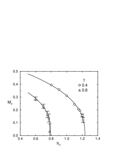
FIG. 5.: The dependence of the spontaneous magnetization on the strength of the random magnetic field $h_{0}$. The data points were fitted by the formula $M_{0}=D\times(h_{c}-h_{0})^{\beta}$.

The phase diagram is plotted in Fig. (4). The critical line (the one passing through the triangle symbols which correspond to our numerical results) is well approximated by the equation

$$h_{c}(\gamma)=h_{c}(0)(1-\gamma^{2})^{\varrho}$$ (11)

where $h_{c}(0)={\rm e}/2$ and $\varrho=0.52\pm 0.01$, very close to $1/2$. Thus the effect of quantum fluctuations in the Griffiths’ region around the critical point is such as to increase the effective strength of the random field. In other words, as the magnetic order is weakened by quantum fluctuations, a weaker random field $h_{0}$ is needed to drive the system to the paramagnetic phase. We point out that the critical field strength vanishes for $\gamma\to 1$, where a different critical behavior sets in [cf. Eq. (10)], controlled by the corresponding critical point.

In the language of SW theory quantum fluctuations lead to a renormalized effective Hamiltonian. The result (10) indicates that the field $S_{\ell}^{x}$ is renormalized as ${\tilde{S}}_{\ell}^{x}=(1-\gamma^{2})^{\vartheta}S_{\ell}^{x}$ at $h_{0}=0$. This in turn leads to an effective Ising-like model with renormalized coupling constant $J_{\gamma}=J(1-\gamma^{2})^{2\vartheta}$. Thus the result (11) indicates that the increase in the strength of random field due to quantum fluctuations is entirely due to a reduction of the coupling constant, while the coupling to the random field is not renormalized, so that the scaling law $\varrho=2\vartheta$ holds. In other words, the interference of the two critical behaviors leads to the relation $(2M_{0})^{2}=2h_{c}/{\rm e}$, i.e. the ratio $M_{0}^{2}/h_{c}=1/2{\rm e}$ is independent of $\gamma$.

To check the consistency of the phase diagram we have calculated the energy gap $G$ between the ground state and the first excited state, which provides an independent determination of the critical point. Indeed, randomness tends to fill in the gap, which should become zero at criticality. This is a property, which is easier to calculate, compared to the spontaneous magnetization, because it can be calculated at zero uniform magnetic field and no extrapolation for $h_{x}\to 0$ is needed. However, unlike the ground-state properties, the properties of the excited states require the full extrapolating procedure $N_{\rm RG}\to\infty$, $s\to\infty$, to be properly determined, even in the Ising limit. Indeed the energy gap depends strongly on the number $s$ of states kept in the DMRG procedure for all $\gamma$. Some examples are shown in Fig. 6, in the absence of randomness. It is seen that, once the correct extrapolation procedure is adopted, the DMRG reproduces the exact result (3) within good accuracy.

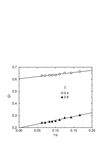
FIG. 6.: The dependence of the energy gap on the inverse number of states kept in the DMRG truncating procedure. The system size is up to 404 sites, $h_{x}=0$, $h_{0}=0$. The straight lines are fits of the form $G=a+b/s$, where $a=0.605\pm 0.003$ for $\gamma=0.4$ and $a=0.197\pm 0.004$ for $\gamma=0.8$.

We have calculated the energy gap $G$ for different $\gamma$ and $h_{0}$ (Fig. 7). As $h_{0}$ increases, $G$ is reduced from its initial value (3) and is driven to zero as the critical point is approached. The results for the gap are in agreement with the results obtained from the spontaneous magnetization data (cf. the triangles in the Fig. 4). The curves are exponentially flat near criticality so that the critical points are much more accurately determined from the magnetization curves. However, once $h_{c}$ is determined from magnetization data, the data corresponding to $-1/\ln(G/G_{0})$ collapse near criticality on one curve as a function of $1-h_{0}/h_{c}$, as shown in the inset of the Fig. 7.

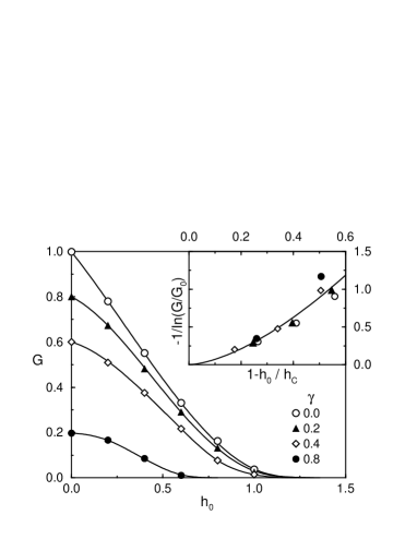
FIG. 7.: The dependence of the energy gap on the strength of the random field $h_{0}$. The system size is above 200 sites, $h_{x}=0$. The average is performed over 500 realizations of the random field. The inset shows rescaled data, and the solid curve is $-1/\ln(G/G_{0})=K(1-h_{0}/h_{c})^{\lambda}$ with $K=2.6\pm 0.4$ and $\lambda=1.6\pm 0.2$. $G_{0}$ denotes the gap in the absence of randomness, Eq. (3).

So far, we have discussed the procedure to obtain the critical behavior of the anisotropic $XY$ model in a random field, and have studied those quantities which vanish at criticality. Now we analyze the correlation length and we look for the nearly critical behavior at a (large) fixed system size and a given number of states in the truncation procedure kept. In particular, since there is a great deal of analysis on finite-size effects in approximate numerical calculations for models near criticality, we concentrate on the distinguishing feature of the DMRG method, i.e. the effect of the truncation of the Hilbert space. Thus we calculated both the connected and nonconnected two-point spin-spin correlation functions along the easy axis of magnetization

$$C_{j}^{t}(r) = 4\left[\langle S_{0}^{x}S_{r}^{x}\rangle-\langle S_{0}^{x}\rangle\langle S_{r}^{x}\rangle\right]$$ (12)

$$C_{j}(r) = 4\langle S_{0}^{x}S_{r}^{x}\rangle,$$ (13)

where $\langle\,\cdot\,\rangle$ stands for the quantum expectation value in the ground state, for any given realization $j$ of the random field, and we are using here an abbreviated notation with respect to Eq. (8). A factor of 4 in the definition of $C_{j}(r)$ was introduced to allow for a direct comparison with Ref. [7] in the Ising limit $\gamma=0$. We point out that, for a given realization of the random field, $\langle S_{0}^{x}\rangle$ and $\langle S_{r}^{x}\rangle$ are different, and neither of them is equal to the magnetization given by Eq. (8), due to the lack of translational invariance.

We used a method which is slightly different from (but essentially equivalent to) the method described, e.g., in Ref. [1]. We grew the system up to a size of $\sim 400$ sites, while storing the truncated spin operators for the different sites of the chain. The typical $C_{j}^{t}(r)$ should decay exponentially with a correlation length $\xi$.[7] The plot of the average over disorder $N_{c}^{-1}\sum_{j=1}^{N_{c}}\ln C_{j}^{t}(r)$ as a function of the distance $r$ allows then to extract the harmonic

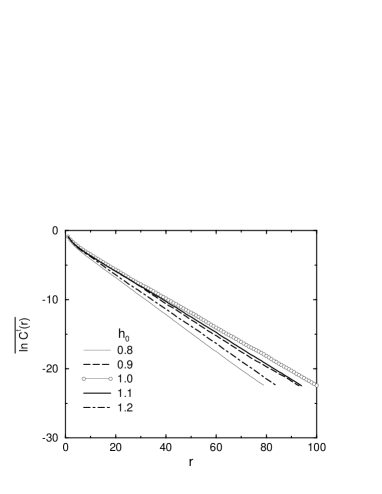
FIG. 8.: The average (over 500 configurations) of the logarithm of the connected correlation function for $\gamma=0.8$. The typical correlation length $\xi$ is calculated as the negative inverse slope of these curves.

average of the correlation length from the slope of the linear behavior at large $r$ (see, e.g., Fig. 8). By plotting the $\xi$ vs $h_{0}$ for each $\gamma$ (Fig. 9), we obtained the peaks that indicate the would-be critical point. As it is evident, the peaks are rather broad, and the correlation lengths rather short, due to the truncation of the Hilbert space, but the position of the maximum can be extracted with a good accuracy, and we found $h_{\rm peak}=1.40\pm 0.05$ for $\gamma=0.0$, $h_{\rm peak}=1.25\pm 0.05$ for $\gamma=0.4$, and $h_{\rm peak}=1.00\pm 0.05$ for $\gamma=0.8$. We checked that increasing the number of states $s$ kept in the truncating procedure leads to narrower peaks which shift towards the critical values $h_{c}(\gamma)$ that were obtained from the spontaneous magnetization data in the infinite-size and $s\to\infty$ limit.

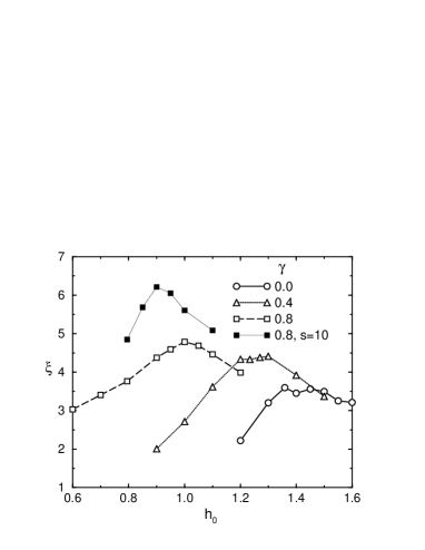
FIG. 9.: The dependence of the typical correlation length $\xi$ on the strength of the random magnetic field $h_{0}$. There were $s=8$ states kept in the truncation procedure for the white data points.

To see how close to criticality the system is at the peaks of the correlation lengths we looked for a typically critical property of the correlation functions. In Fig. 10 we plotted the average over the realizations of the random field of the logarithm of the correlation function (13), $\overline{\ln C(r)}\equiv N_{c}^{-1}\sum_{j=1}^{N_{c}}\ln C_{j}(r)$ as a function of $\sqrt{r}$, since such a behavior is expected at criticality.[1, 7] Our result shows that the curves are very sensitive to the value of $h_{0}$, and bend upwards when $h_{0}$ is smaller than some particular value $\hat{h}$ or downwards when $h_{0}>\hat{h}$. The best fit to linear behavior is found at $\hat{h}=1.44$ for $\gamma=0.0$, $\hat{h}=1.30$ for $\gamma=0.4$, and $\hat{h}=1.03$ for $\gamma=0.8$. These values and the corresponding $h_{\rm peak}$, obtained from the $\xi$ vs $h_{0}$ curves, coincide within the error bars. Thus the truncated Hilbert space embodies the critical behavior of the system in a self-consistent though approximate way. Increasing the size of the Hilbert space improves the accuracy in the description of the critical properties until the only limitation to a fully developed criticality is the finite size of the system. It is perhaps important to remark that the extrapolating procedure proposed in Sec. III to extract the spontaneous magnetization may also be applied to the correlation functions. The only difference is that much more computational time and memory is required to calculate and store the data which refer, for a given distance $r$, to different system sizes, different number of states $s$, and different random field realizations.

FIG. 10.: The average of the logarithm of the nonconnected correlation function. The curves correspond to the following strengths of the random magnetic field (from top to bottom): $h_{0}=1.25;\ 1.44;\ 1.65$ for $\gamma=0.0$ (solid lines), $h_{0}=1.1;\ 1.3;\ 1.5$ for $\gamma=0.4$ (dot-dashed lines), and $h_{0}=0.8;\ 1.03;\ 1.2$ for $\gamma=0.8$ (dashed lines).

V Conclusions

In summary, we analyzed some properties of the spin-1/2 quantum anisotropic $XY$ chain in a transverse random magnetic field by means of the density-matrix renormalization group. The dependence of the magnetization on the uniform magnetic field $h_{x}$, the strength of the random magnetic field $h_{0}$ and the factor of anisotropy $\gamma$ was obtained. The order-disorder phase-transition line was determined [Eq. (11)] and the phase diagram was drawn. The energy gap between the ground state and the first excited state was investigated as well. The dependence of the gap on both the strength of the random field $h_{0}$ and the factor of anisotropy was obtained. The gap vanishes at the phase transition, determined independently from magnetization data, and reproduces the correct limiting value (3) as the strength of the random field is reduced. Finally we calculated the connected and nonconnected two-point spin-spin correlation functions along the easy axis of magnetization. We studied in particular the asymptotic behavior for large distances at criticality, and found that the $\sqrt{r}$-behavior found at $\gamma=0$[1, 7] persists for $\gamma>0$.

The critical properties are remarkably the same for all $\gamma<1$, providing clear numerical evidence for universality, i.e. models with different values of the factor of anisotropy $0\leq\gamma<1$ all belong to the same universality class as the spin-1/2 quantum Ising chain in a transverse random magnetic field.

The main advantages of the method used in this paper to investigate the properties of a random quantum system, with respect to other numerical methods have been discussed in our previous paper. [1] Here we wish to comment in deeper detail on the specific technical problem which was dealt with in this paper. Indeed, in the present case, the density-matrix renormalization-group approach requires a particular care, due to the interplay of randomness, finite-size effects, and because the consequences of truncation of the Hilbert space are enhanced by the presence of quantum fluctuations (with respect to an Ising-like ground state) as $\gamma$ is increased. This effect is most easily seen in the gradual spread of the eigenvalues of the density matrix, i.e. in the increasing importance of including more states in the truncating procedure, in order to obtain an accurate description of the system. However a reliable protocol was discussed in this paper, which takes care of all those aspects on equal footing, allowing us to obtain physical results which are very robust with respect to “local” variations of the extrapolating procedures.

Criticism was often raised against the use of the DMRG in the investigations of random systems (see, e.g. Ref. [12]), and some modifications of the DMRG procedure were proposed to deal with randomness.[13] The authors essentially refer to the failure in accommodating sudden changes of the ground state within a truncated basis for the Hilbert space. These objections are appropriate, in principle, and suggest a careful analysis of the stability of the DMRG results as the size of the basis is enlarged. In this paper we showed that this analysis is possible, and the objections may be overcome.

- [1] A. Juozapavičius, S. Caprara, and A. Rosengren, Phys. Rev. B 56, 11097 (1997).
- [2] E. Lieb, T. Schultz, and D. Mattis, Ann. Phys. 16, 407 (1961).
- [3] It is worth mentioning that the model is nonintegrable when is finite.
- [4] We adopt in our paper a notation which is different from the one adopted in Ref. [2] in both the definition of the spin operators, and of the anisotropy factor. All the results have been consistently translated into our notation.
- [5] B. M. McCoy and T. T. Wu, Phys. Rev. 176, 631 (1968).
- [6] R. Shankar and G. Murthy, Phys. Rev. B 36, 536 (1987).
- [7] D. S. Fisher, Phys. Rev. B 51, 6411 (1995).
- [8] The notation here is different from both the notation adopted in our previous paper[1] and the notation used in Ref. [7]. This is due to the fact that the model discussed in the present paper is known in the literature as the model, whereas the Ising limit is usually discussed within a model. Thus the and axes of Refs. [1, 7] have been interchanged here.
- [9] R. B. Griffiths, Phys. Rev. Lett. 23, 17 (1969).
- [10] A. P. Young and H. Rieger, Phys. Rev. B 53, 8486 (1996).
- [11] S. R. White, Phys. Rev. Lett. 69, 2863 (1992), Phys. Rev. B 48, 10345 (1993).
- [12] N. V. Prokof’ev and B. V. Svistunov, Phys. Rev. Lett. 80, 4355 (1998).
- [13] K. Hida, J. Phys. Soc. Jpn. 65, 895, (1996).